Steel Plate Surface Defect Detection Based on Dataset Enhancement and Lightweight Convolution Neural Network

Abstract

In the production and manufacturing industry, factors such as rolling equipment and processes may cause various defects on the surface of the steel plate, which greatly affect the performance and subsequent machining accuracy. Therefore, it is essential to identify defects in time and improve the quality of production. An intelligent detection system was constructed, and some improved algorithms such as dataset enhancement, annotation and lightweight convolution neural network are proposed in this paper. (1) Compared with the original YOLOV5 (You Only Look Once), the precision is 0.924, and the inference time is 29.8 ms, which is 13.8 ms faster than the original model. Additionally, the parameters and calculations are also far less than YOLOV5. (2) Ablation experiments were designed to verify the effectiveness of the proposed algorithms. The overall accuracy was improved by 0.062; meanwhile, the inference time was reduced by 21.7 ms. (3) Compared with other detection models, although RetinaNet has the highest accuracy, it takes the longest time. The overall performance of the proposed method is better than other methods. This research can better meet the requirements of the industry for precision and real-time performance. It can also provide ideas for industrial detection and lay the foundation for industrial automation.

1. Introduction

In the complicated process of industrial production, any abnormality leads to product defects. For instance, the rolling equipment and processes may cause scratches, inclusions, patches and so on. Those defects not only affect the corrosion resistance, wear-resistance and fatigue strength of the steel plate but also have a profound impact on the accuracy of subsequent processing [1]. Identifying the defect patterns of abnormal products in time is an effective way to improve the production quality and efficiency, so defect detection has very important research significance [2,3].

Early product defect recognition is mainly carried out through machine learning, such as support vector machine [4,5] and back-propagation network [6,7]. Gao [8] extracted key feature information from GS-PCA and input it to SVM (Support Vector Machine) for classification. Xu [9] established multiple SVM models through Ada Boost to classify sonar images with low resolution and noise. However, these above-mentioned methods greatly lie on the quality of manually extracting features, which directly affects the recognition accuracy. Deep learning based on convolutional neural networks has very powerful feature extraction capabilities and sufficient flexibility in the field of industrial inspection [10,11,12,13]. Hao [14] used the deformable convolution enhanced network to extract complex features from steel surface defects, based on NEU-DET (Detection dataset of Northeastern University), with 0.805 of precision and 23 ms of inference speed. The accuracy is low and needs to be improved. Guan [15] pretrained the steel surface defect classification task with VGG19, then evaluated the characteristic image quality with SSIM (Structual Similarity) and decision tree; the accuracy was 91.66. The open dataset was directly used, and the technology of image acquisition, preprocessing and dataset annotation was not studied in this research. Feng [16] added FcaNet (Frequency Channel Attention Networks) and CBAM (Convolutional Block Attention Module) on the basis of ResNet, the dataset contained 1360 images, and the parameter quantity was 26.038 M. The dataset was small, and the model was large. Yang [17] used YOLOV5X (You Only Look Once) to detect steel pipe welding defects. The accuracy was 98.7, but the inference speed was 120 ms, which did not meet the real-time industrial requirements. Konovalenko [18] detected three kinds of defects based on ResNet50 and ResNet152. The average accuracies were 0.880 and 0.876, respectively. There were few defect types and low accuracy.

In summary, the above methods have inadequacies such as small datasets, few defect types, low accuracy and long time consumption. (1) In order to improve the model performance, the lightweight MobilenetV2 was used to improve the YOLOV5, and the CBAM attention module was added to optimize the accuracy of target detection. The upgraded YOLOV5 reduces the parameters and calculations and improves the inference speed. (2) In the highly automated production scenarios, the yield of products is particularly high, so images with defects are not easy to obtain. In order to increase samples, the collected images were firstly expanded, and then a defect dataset was created by combining the NEU-DET and the dataset collected in this paper. Moreover, due to the complex environment of the field, the quality of the acquired image was unstable, so it was difficult to annotate the dataset and classify the defects. Image enhancement before detection can effectively improve recognition accuracy. However, there is no image preprocessing in these methods. An improved MSR (Multi-Scale Retinex) algorithm was proposed to improve the quality of images. (3) Creating datasets by manually labeling the bounding box is slow and laborious. Therefore, an adaptive bounding box extraction algorithm is proposed in this paper to obtain the target regions automatically, which can greatly assist the dataset annotation. A steel plate defect detection system was established in this paper to collect and analyze the images and record and store the detection results. The above-proposed algorithms were embedded in the monitoring center of the system.

2. Overall Framework and Algorithm Structure of Steel Plate Defect Detection

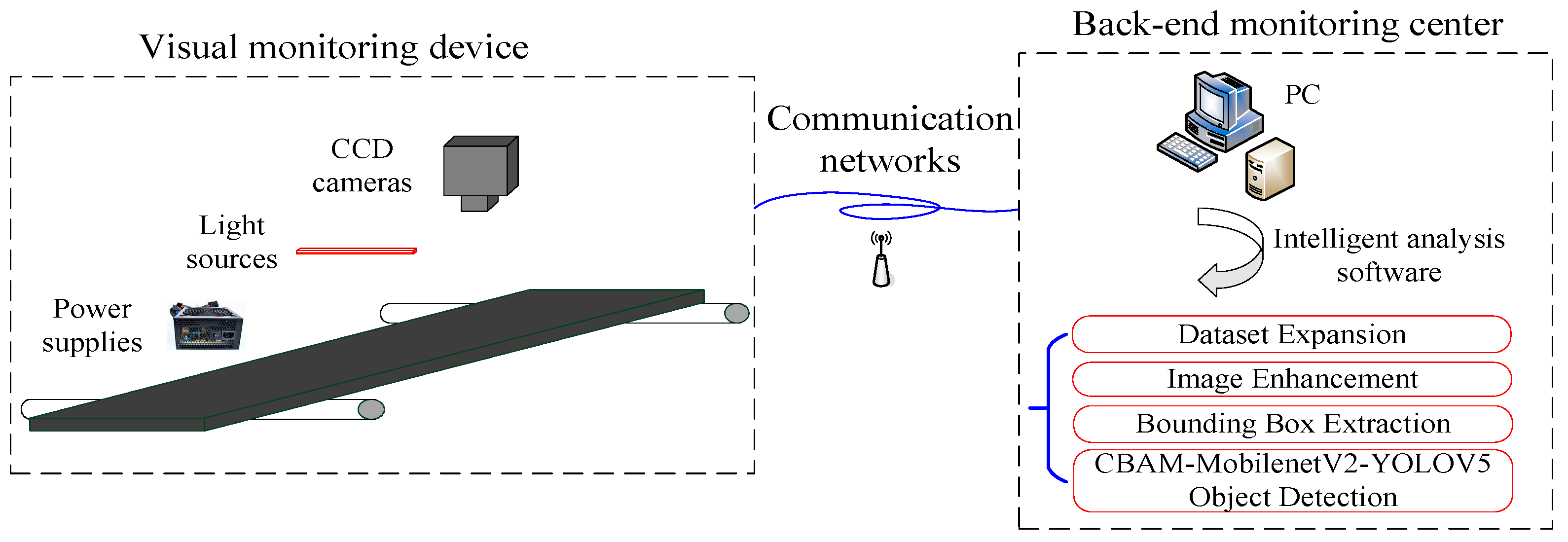
The overall framework of the system is shown in Figure 1; it mainly includes a visual monitoring device, communication networks and a back-end monitoring center. The visual monitoring device mainly consists of CCD cameras, light sources and power supplies. After the steel plate is rolled, the surface images are collected by the visual monitoring device and transmitted to the back-end monitoring center through the communication network. The received images are processed by intelligent analysis software and various embedded intelligent algorithms. The detection results can be recorded and stored to evaluate the quality of the whole steel plate.

The algorithm structure is shown in Figure 2. Firstly, the collected defect images were expanded, and an improved MSR algorithm based on adaptive weight calculation was proposed to enhance the images. Then an adaptive bounding box extraction algorithm for the defect dataset was proposed. The position of the target can be automatically obtained based on image block and pixel difference algorithms, which can assist the dataset annotation. Finally, a deep learning detection model was designed. The baseline network adopts YOLOV5 (You Only Look Once), the backbone part was replaced by the lightweight network MobilenetV2, and the attention module CBAM (Convolutional Block Attention Module) was added for adaptive feature optimization. NEU-DET (Detection dataset of Northeastern University) and self-processed images together constitute the defect dataset to train and test the lightweight YOLOV5 model.

3. Dataset Preparation

3.1. Image Expansion

In some highly automated industrial production scenarios, the product yield is high, and it is difficult to collect defect samples. In addition, defects are caused by uncontrolled factors in the production process; collecting them in various forms is a challenging task. Therefore, it is necessary to expand the defect samples. Five kinds of defects were mainly detected in this paper: inclusion, scratch, scab, pitted surface and patch. Images were processed by rotation, mirror and Gaussian convolution, as shown in

Table 1. Image expansion.

Extension Method	Inclusion	Scratch	Scab	Pitted Surface	Patch
Original image
Mirror
Rotate 90°
Rotate 180° + convolution
Rotate 90° + mirror

. One thousand five hundred defect images can be obtained after expansion.

3.2. Improved MSR Image Enhancement

The detection effect of machine vision is affected by the ambient light, and the non-uniformity of the illumination has a significant impact on the measurement. The adjustment process is quite complicated, even after the adoption of the strict illumination method, which still affects the illumination intensity of the object surface. At present, the main method to reduce the influence of external illumination is image preprocessing, which can reduce the influence of the illumination to a certain extent and improve the image quality. The MSR algorithm (Multi-Scale Retinex) [19,20] is a multi-scale algorithm that divides an image into reflected images and incident images. By combining the multi-scale filtering results, the corresponding reflection component can be calculated as the enhanced image. However, the scale weight W_k is set manually, which is greatly affected by subjective factors. Therefore, an improved MSR algorithm based on adaptive weight calculation was proposed, by which the weight can be automatically determined by calculating the proportion of information entropy [21,22] at different scales. The mean gray of the neighborhood and the pixel gray in the image were selected to form the feature binary (i, j), where i represents the gray value of the pixel (0 ≤ I ≤ 255), j represents the neighborhood mean gray (0 ≤ j ≤ 255) and P_ij represents the proportion of the feature binary (i, j):

$$P_{ij}=N\left(i,j\right)/M$$

(1)

where N(i, j) represents the frequency of the feature binary (i, j), and M represents the total number of pixels in the image.

Then the two-dimensional entropy is:

$$H=-{\displaystyle \sum _{i=0}^{255}{\displaystyle \sum _{j=0}^{255}{P}_{ij}}\log P_{ij}}$$

(2)

Therefore, the calculation formula of scale weight is as follows:

$$W_k=\frac{H_k}{{\displaystyle \sum _{l=1}^K{H}_l}}$$

(3)

where H_k represents the two-dimensional information entropy of scale k, and K represents the total number of scales. The defect images are processed by the improved MSR, and the traditional MSR algorithm is used for comparison. The enhancement results are shown in

Table 2. MSR and improved MSR image enhancement.

Data Enhancement	Scratch	Inclusion	Patch	Scab	Pitted Surface
Original image
MSR
Improved MSR

; the improved MSR algorithm has less background interference and a clear target edge.

In order to quantify the enhancement effect, the gray standard deviation and information entropy of original images and improved MSR enhanced images were calculated. As shown in

Table 3. Gray feature calculation of original defect images and improved MSR enhanced images.

Feature	Scratch		Inclusion		Patch		Scab		Pitted Surface
	Original Image	This Paper	Original Image	This Paper	Original Image	This Paper	Original Image	This Paper	Original Image	This Paper
Standard deviation	21.62	31.87	10.60	21.40	23.52	31.16	15.05	21.13	13.63	28.60
Information entropy	6.39	6.51	5.39	6.21	6.13	6.47	5.64	5.94	5.76	6.78

, the features of enhanced images are both larger than that of original images, which indicates that the proposed enhancement algorithm improves the overall contrast and the amount of the image information.

3.3. Adaptive Target Bounding Box Extraction

In order to overcome the subjectivity of manual annotation, an adaptive bounding box extraction method based on image block and pixel difference was proposed. As shown in Figure 3, the position information of the rectangular box can be automatically obtained, and the annotation of the dataset can be assisted.

(1)

Image block [23,24]: the image is divided into three parts by row: I1, I2 and I3, and three parts by column: I4, I5 and I6, as shown in Figure 4;

(2)

Calculation of second-order difference matrix: the difference between this row (column) and the next row (column) minus the difference between this row (column) and the previous row (column), which are arranged in order at the corresponding position of the previous row (column) [25,26].

The row difference is:

$$MD2=[M(3,:)+M(1,:)-2M(2,:);\dots ;M(m,:)+M(m-2,:)-2M(m-1,:)]$$

(4)

where MD2 is a matrix of (m − 2) ∗ n.

The column difference is:

$$ND2=[N(:,3)+N(:,1)-2N(:,2);\dots ;N(:,n)+N(:,n-2)-2N(:,n-1)]$$

(5)

where ND2 is a matrix of m ∗ (n − 2).

The mean value of I1, I2 and I3 are calculated by column, and then the column second-order difference can be calculated from the horizontal direction. As shown in Figure 5a, the column second-order difference of the three blocks is represented by different colors, which constitute a difference matrix ND2. Similarly, the mean value of I4, I5 and I6 are calculated by row, and the row second-order difference can be calculated from the vertical direction. As shown in Figure 5b, the row second-order difference of the three blocks consists of a difference matrix MD2.

(3)

Boundary calculation: A boundary calculation method is proposed in this paper, which considers the distribution difference of the targets in each sub-block.

(1) Calculate the left and right boundaries: Divide the matrix ND2 into the first third of the columns, the middle third of the columns and the last third of the columns: A. If there are image targets in all three blocks I4, I5 and I6, the first third of the columns of ND2 are taken to calculate the left boundary, and the last third of the columns are taken to calculate the right boundary. B. If there are image targets in I4 and I5, the first third of the columns of ND2 are taken to calculate the left boundary, and the middle third of the columns are taken to calculate the right boundary. C. If there are image targets in I5 and I6, the middle third of the columns of ND2 are taken to calculate the left boundary, and the last third of the columns are taken to calculate the right boundary. D. If only the I4 part has the image target, the first third of the columns of ND2 are taken to calculate the left and right boundaries, respectively. E. If only the I5 part has the image target, the middle third of the columns of ND2 are taken to calculate the left and right boundaries, respectively. F. If only the I6 part has the image target, the last third of the columns of ND2 are taken to calculate the left and right boundaries, respectively.

As shown in Figure 4b, after the image is divided by column, there are image targets only in I4 and I5, so the first third and the middle third of the columns of matrix ND2 are extracted. For the first third of the columns, as shown in Figure 6, the column numbers of the first maximum value from the left of each row are calculated, and the minimum value of 37 is taken as the left boundary minL. Similarly, for the middle third of the columns, the column numbers of the first maximum value from the right of each row are calculated, and the maximum value 74 is taken as the right boundary maxR.

(2) Calculate the upper and lower boundaries: Divide the matrix MD2 into the first third of the rows, the middle third of the rows and the last third of the rows. The calculation principle is the same as above, and the upper and lower boundaries are calculated according to the target distribution of three blocks. As shown in Figure 4a, there are image targets in I1, I2 and I3, so the first third and the last third of the rows of matrix MD2 are extracted. As shown in Figure 7, the row numbers of the first maximum value from top to bottom of each column in the first third of the rows are calculated, and the minimum value 1 is taken as the upper boundary minU. Similarly, the row numbers of the first maximum value from bottom to top of each column in the last third of the rows are calculated, and the maximum value 191 is taken as the lower boundary maxD.

The minL, maxR, minU and maxD were taken as the four boundaries of the bounding box. The annotation results of different defect images are shown in Figure 8. One thousand five hundred enhanced defect images were annotated by the above method, with an average annotation time of 285 ms and an average IOU of 0.93.

4. Classification Network Design

4.1. Model Structure

As shown in Figure 2, an improved CBAM-MobilenetV2-YOLOv5 model is proposed in this paper. The backbone network of YOLOV5 was replaced by the lightweight network MobilenetV2, and the attention module CBAM was added to the feature extraction part for adaptive feature optimization.

(1)

YOLOV5

YOLOV5 [17,27,28] mainly consists of Backbone, Neck and Head. Mosaic data enhancement, adaptive anchor box calculation and adaptive image scaling were added to the data input part to process the data and increase the detection accuracy. In Backbone, the Focus and CSP1_X structures were mainly used. The Focus structure was carried out for slicing operations, and the size of the feature map was reduced by increasing the dimension without losing any information, which can obtain the double downsampling feature map. A residual structure was added to CSP1_X to enhance the gradient value during the back-propagation process between layers, effectively preventing the gradient from disappearing when the network is deepened. The CSP2_X structure was adopted in the Neck to reduce the amount of calculation and strengthen the fusion ability of network features. A feature pyramid was designed in the Neck layer to transmit information from top to bottom, and a path aggregation structure was used to transmit localization information. The loss function of the bounding anchor box in the Head is GIOU_Loss, and the weighted NMS (Non-maximum Suppression) operation was used to screen multiple target anchor boxes and improve the recognition accuracy.

(2)

MobilenetV2

Different from the original residual structure, an inverse residual structure was adopted in MobilenetV2 [29,30]. It first increases the dimension, then performs depthwise convolution calculations and finally reduces the dimension. The last ReLU6 layer was replaced by the Linear, which reduces the loss of features and obtains better detection results. The depthwise convolution module is shown in Figure 9. There are three filters, and each filter is a 3 × 3 convolution kernel.

(3)

CBAM

The CBAM attention [31,32] was used in the model to optimize the target detection accuracy and strengthen the focus on the detected targets. It consists of two independent sub-modules: the channel attention module CAM and the spatial attention module SAM, which perform attention in the channel and space dimensions, respectively. When given a feature map, the attention map can be sequentially inferred by the CBAM module along two independent dimensions, and then the attention map is multiplied with the input feature map for adaptive feature optimization.

4.2. Evaluation Indicator

The IOU between the predicted bounding box and the ground truth bounding box can be calculated as follows [33,34]:

$$IOU=\frac{area(B_p\cap B_{gt})}{area(B_p\cup B_{gt})}$$

(6)

where B_p is the predicted bounding box, B_gt is the ground truth bounding box. IOU is the area of intersection of B_p and B_gt divided by the area of union. The larger the IOU, the more consistent the predicted box and the truth box.

(1)

Accuracy P and recall R

The calculation formulas are as follows [17]:

$$P=\frac{TP}{TP+FP}=\frac{TP}{all\hspace{0.17em}detections}$$

(7)

$$R=\frac{TP}{TP+FN}=\frac{TP}{all\hspace{0.17em}ground\hspace{0.17em}truths}$$

(8)

where TP indicates a correct detection, IOU ≥ threshold. FP indicates an error detection, IOU < threshold. FN means the true value has not been detected, that is, “missed detection”. TN indicates there is no true value, and it was not detected.

(2)

AP (average precision) and mAP (mean average precision)

Suppose there are M positive samples in the total N samples. After ranking according to the confidence, there are M Recall values from Top-1 to Top-M, which are (1/M, 2/M, …, M/M), respectively. For each Recall value, the maximum P can be calculated from r ≥ Recall. The AP is the average value of these P, which indicates the quality of the trained model in the current category. The AP for each category and the mean value mAP for all categories can be calculated.

5. Experiment Analysis

5.1. Monitoring Platform and Configuration Parameters

The visual monitoring platform is shown in Figure 10. It includes CCD cameras, light sources, power supplies and so on.

The parameters of the high-speed industrial camera are shown in

Table 4. Camera parameters.

Camera	Size	Pixel	Resolution	Frame rate	Interface
WP-UT030	29 × 29 × 29 mm	300 thousand	640 × 480 pixels	815FPS	USB 3.0

. It can be connected with MATLAB, Halcon and other third-party software. The weight and volume are small, which is suitable for industrial automation equipment with limited installation space. The light source is coaxial light source WP-CO250260, the luminous surface is 264 × 263 mm and the power is 33 W. It is applicable to the detection of scratches, cracks and other defects on the reflective metal surface. In the experimental environment, a camera and a light source were used to collect images. In the actual production field, three to five groups of cameras and light sources were set according to the monitoring range. The position and angle of the camera and the light source can be adjusted with the corresponding brackets. The camera was installed on the top of the steel plate and perpendicular to the steel plate plane. The light source was directly installed above the steel plate, and the brightness can be adjusted according to the actual demand to make the illumination on the image surface as uniform as possible.

The hardware and software configuration information of the algorithm are shown in

Table 5. Hardware and software configuration information.

Name	Configuration Information
Operation system	Ubuntu 18.04, 64 bit
CPU	Intel(R) Core(TM) i5-10210Y
GPU	NVIDIA GeForce GTX 1080 Ti, 11 G
Language	Python 3.7.9
Deep learning framework	Pytorch 1.7.1

; the experiment was carried out in the Ubuntu system, the GPU was NVIDIA GeForce GTX 1080 Ti and the Pytorch deep learning framework was used. The initial learning rate was set to 0.01, the momentum coefficient was 0.937, the batch size was 32, the number of training categories was set to 5, and the epoch was set to 200.

5.2. Dataset

Six kinds of defects were included in the open dataset NEU-DET: rolled in scale, patches, cracks, pitted surface, inclusion and scratches. Defects common to this paper are patches, pitted surface, inclusions and scratches. Therefore, a defect dataset is formed by combining 1200 samples of these four defects in NEU-DET and 1500 samples collected in this paper, with a total of 2700 samples, including 600 patches, 600 pitted surfaces, 600 inclusions, 600 scratches and 300 scabs. Each image had three channels, and the pixel size was 200 × 200. All samples were randomly divided into train and test in a ratio of 7:3, which contains 1890 training images and 810 testing images.

5.3. Experimental Results and Analysis

After each epoch, the test was performed on the model. The precision, recall and loss curves of the test dataset are shown in Figure 11. After 150 epochs, each curve gradually tends to converge. The parameters of the best epoch were used as the model parameters. The classification precision P, recall R and average precision AP of each defect are shown in

Table 6. Classification evaluation indicators of each defect category.

Defect Category	P	R	AP
Patches	0.986	0.957	0.977
Pitted surface	0.949	0.891	0.955
Inclusion	0.936	0.918	0.962
Scratches	0.98	0.844	0.949
Scabs	0.784	0.615	0.777
All	0.927	0.845	0.924

. The AP of patches and inclusions are higher, both above 0.96, because they are labeled more accurately, and the contrast between the target and the background is clearer. The AP and R of scabs are poor because, on the one hand, the scab is a convex defect, the convex part has reflection, and the color of the whole target is close to the background. On the other hand, the number of samples collected is less than other defects, which affects the accuracy of feature learning. Overall, the average precision of five defects was 0.924, and the detection effect was good.

In the detection results, the confidence distribution of each target is shown in Figure 12. The range of 0.2–0.4 means 0.2 ≤ confidence < 0.4, 0.4–0.6 means 0.4 ≤ confidence < 0.6, 0.6–0.8 means 0.6 ≤ confidence < 0.8, 0.8–1.0 means 0.8 ≤ confidence ≤ 1.0. The confidence of most defect targets are between 0.8 and 1.0, and a few are between 0.2–0.4 and 0.4–0.6.

5.3.1. Compared with Original YOLOV5

The dataset in Section 5.2 was input into the original YOLOV5 and the improved YOLOV5, respectively. Figure 13 shows the [email protected] and [email protected]:.95 in the epoch process of two models, both models tend to be stable after 100 epochs, and the accuracy of this paper is slightly lower than the original model. The backbone part was replaced by the lightweight net MobilenetV2, which reduces the number of model parameters at the cost of losing some accuracy.

Table 7. Performance comparison before and after improvement.

Model	[email protected]	[email protected]:.95	Params (M)	Flops (G)	Inference Time (ms)
YOLOV5	0.932	0.608	26.80	15.82	43.6
This paper	0.924	0.600	13.91	8.95	29.8

shows the average precision [email protected] and [email protected]:.95, amount of parameters, amount of calculations and inference speed of two models. The precision of this paper was 0.924, which is 0.008 lower than the original model. However, the Params, Flops and Inference time are far less than the YOLOV5. The comprehensive performance was improved.

5.3.2. Ablation Experiments of the Proposed Algorithm

Three improved algorithms are mainly proposed in this paper: improved MSR image enhancement, automatic target bounding box annotation and lightweight YOLOV5. In order to verify the value of the proposed module, ablation experiments were designed to test the model by gradually adding modules. As shown in

Table 8. Ablation experiments of the proposed algorithm.

Improved MSR Image Enhancement	Automatic Bounding Box Annotation	Lightweight YOLOV5	[email protected]	Inference Time (ms)
×	×	×	0.862	51.5
×	×	√	0.847	37.2
√	√	√	0.924	29.8

, by using the lightweight YOLOV5 module, the accuracy decreased by 0.015, but the inference time was reduced by 14.3 ms. By adding the improved MSR image enhancement and automatic target box annotation modules, the accuracy was improved by 0.077, and the inference time was reduced by 7.4 ms. The overall accuracy of the three modules was improved by 0.062, and the inference time was reduced by 21.7 ms. The image enhancement algorithm proposed in this paper can effectively improve the image quality and is conducive to target annotation, feature extraction and learning. The overall performance of the algorithms proposed in this paper is superior.

5.3.3. Compared with Other Models

In order to verify the algorithms proposed in this paper, SSD [35], Faster R-CNN [10] and RetinaNet [36] were used for comparative experiments. As shown in Figure 14, RetinaNet has the highest accuracy of 0.941, but its inference time is 84.5 ms, which is the most time-consuming. The precision of this paper is 0.924, but the time is 29.8 ms, and the overall performance is better than other models. It not only has high precision, but also meets the real-time requirements of industrial detection better.

5.4. Field Running Tests

The intelligent detection system was tested in the equipment operation field of the China Heavy Machinery Research Institute. The monitoring field is shown in Figure 15. Image acquisition and operation status monitoring were carried out for the steel plate in the production process.

As shown in Figure 16, the expert software for intelligent analysis of steel plate defects installed in the monitoring center was developed by combining VC++, MATLAB and Python, in which various intelligent algorithms designed in this paper were embedded. Its functions consisted of load image, image expansion, image enhancement, dataset annotation, model training and defect detection. The processing results of images are displayed on the right side of the interface, and the detection results are displayed below the interface. The visual results and detection data results can be displayed by clicking the corresponding functions. Figure 16a shows the enhancement effect of a scratch image, and Figure 16b shows the detection results of a patch image.

6. Conclusions

This paper proposes a lightweight improved YOLOV5 model and some improved dataset enhancement and adaptive bounding box annotation algorithms for steel surface defect detection. Firstly, an improved MSR algorithm based on adaptive weight calculation was proposed, which can automatically obtain the scale weight by calculating the proportion of information entropy. Compared with the original image and traditional MSR, the image contrast and quality were improved. Secondly, an adaptive bounding box extraction algorithm for steel plate defect datasets was proposed. It obtains the bounding box of the target based on the image block and pixel difference algorithm, which can assist the dataset annotation. The average annotation time was 285 ms, and the average IOU was 0.93. Finally, an improved lightweight YOLOV5 model was designed, and the NEU-DET dataset and the processed images by the proposed algorithm together formed the dataset. (1) Compared with the original YOLOV5, although the accuracy was reduced by 0.008, the inference speed was 29.8 ms, which is faster than the traditional model. Additionally, the parameters and calculations were also far less than YOLOV5. (2) In order to verify the value of the proposed module, ablation experiments were designed by gradually adding modules. The overall accuracy was improved by 0.062, and the inference time was reduced by 21.7 ms. The image enhancement algorithm proposed in this paper can effectively improve the image quality and is conducive to target annotation, feature extraction and learning. (3) Compared with other detection models, the precision of SSD, Faster R-CNN and RetinaNet are 0.686, 0.871 and 0.941, respectively. Although RetinaNet has the highest accuracy, 0.941, its inference time is 84.5 ms, which is the most time-consuming. The precision of this paper is 0.924, but the time is 29.8 ms, which more meets the accuracy and real-time requirements of the industry, and the overall performance is better than other methods. This research can provide ideas for the real-time detection of steel plate defects in industrial environments and lay a foundation for industrial automation.

Although advanced deep learning algorithms and convolutional neural networks were used in this paper to achieve defect detection in the industrial production field, other categories of defects that do not exist in the dataset cannot be correctly identified in the case of limited datasets. The next step is to collect more images of different defects and study more detection algorithms and technologies.

References

- Chen, N.; Sun, J.; Wang, X.; Huang, Y.; Li, Y.; Guo, C. Research on surface defect detection and grinding path planning of steel plate based on machine vision. In Proceedings of the 2019 14th IEEE Conference on Industrial Electronics and Applications (ICIEA), Xi’an, China, 19–21 June 2019; pp. 1748–1753. [Google Scholar]
- Usamentiaga, R.; Garcia, D.F.; de la Calle Herrero, F.J. Real-Time Inspection of Long Steel Products Using 3-D Sensors: Calibration and Registration. IEEE Trans. Ind. Appl. 2018, 54, 2955–2963. [Google Scholar] [CrossRef]
- Qin, Y.R. Steel Surface Quality and Development of Intelligent Detection; Nangang Technology and Management: Taipei, Taiwan, 2020; pp. 32–33. [Google Scholar]
- Gao, Y.; Yang, Y. Classification based on multi-classifier of SVM fusion for steel strip surface defects. In Proceedings of the 32nd Chinese Control Conference, Xi’an, China, 26–28 July 2013; pp. 3617–3622. [Google Scholar]
- Belkacemi, B.; Saad, S. Bearing various defects diagnosis and classification using super victor machine (SVM) method. In Proceedings of the International Conference on Information Systems and Advanced Technologies (ICISAT), Tebessa, Algeria, 27–28 December 2021; pp. 1–7. [Google Scholar]
- Tang, C.; Chen, L.; Wang, Z.; Sima, Y. Study on Software Defect Prediction Model Based on Improved BP Algorithm. In Proceedings of the IEEE Conference on Telecommunications, Optics and Computer Science (TOCS), Shenyang, China, 11–13 December 2020; pp. 389–392. [Google Scholar]
- Li, X.; Zhang, T.; Deng, Z.; Wang, J. A recognition method of plate shape defect based on RBF-BP neural network optimized by genetic algorithm. In Proceedings of the 2014 The 26th Chinese Control and Decision Conference (2014 CCDC), Changsha, China, 31 May 2014–2 June 2014; pp. 3992–3996. [Google Scholar]
- Gao, X.; Hou, J. An improved SVM integrated GS-PCA fault diagnosis approach of Tennessee Eastman process. Neurocomputing 2016, 174, 906–911. [Google Scholar] [CrossRef]
- Xu, H.; Yuan, H. An SVM-Based AdaBoost Cascade Classifier for Sonar Image. IEEE Access 2020, 8, 115857–115864. [Google Scholar] [CrossRef]
- Lu, S.l.; Ma, C.; Hu, H.; Wang, S.F.; Huang, D. Research on surface defect identification of steel plate based on Faster R-CNN. Comput. Program. Ski. Maint. 2021, 110–113. [Google Scholar]
- LI, J.Z.; YIN, Z.Y.; Le, X.Y. Surface defect detection for steel plate with small dataset. Aeronaut. Sci. Technol. 2021, 32, 65–70. [Google Scholar]
- Wang, S. Research on Key Algorithm of Product Surface Defect Detection Based on Machine Vision; University of Chinese Academy of Sciences (Shenyang Institute of computing technology, Chinese Academy of Sciences): Shenyang, China, 2021. [Google Scholar]
- Luo, Q.; Fang, X.; Liu, L.; Yang, C.; Sun, Y. Automated Visual Defect Detection for Flat Steel Surface: A Survey. IEEE Trans. Instrum. Meas. 2020, 69, 626–644. [Google Scholar] [CrossRef] [Green Version]
- Hao, R.; Lu, B.; Cheng, Y.; Li, X.; Huang, B. A steel surface defect inspection approach towards smart industrial monitoring. J. Intell. Manuf. 2021, 32, 1833–1843. [Google Scholar] [CrossRef]
- Guan, S.; Lei, M.; Lu, H. A Steel Surface Defect Recognition Algorithm Based on Improved Deep Learning Network Model Using Feature Visualization and Quality Evaluation. IEEE Access 2020, 8, 49885–49895. [Google Scholar] [CrossRef]
- Feng, X.; Gao, X.; Luo, L. A ResNet50-Based Method for Classifying Surface Defects in Hot-Rolled Strip Steel. Mathematics 2021, 9, 2359. [Google Scholar] [CrossRef]
- Yang, D.; Cui, Y.; Yu, Z.; Yuan, H. Deep Learning Based Steel Pipe Weld Defect Detection. Appl. Artif. Intell. 2021, 35, 1237–1249. [Google Scholar] [CrossRef]
- Konovalenko, I.; Maruschak, P.; Brevus, V. Steel Surface Defect Detection Using an Ensemble of Deep Residual Neural Networks, ASME. J. Comput. Inf. Sci. Eng. 2022, 22, 014501. [Google Scholar] [CrossRef]
- Zhang, Y.Y. Research of Haze Color Image Enhancement Based on Multi-Scale Retinex. Packag. J. 2016, 8, 60–65. [Google Scholar]
- Jang, C.Y.; Kim, Y.H. An energy efficient multi-scale retinex algorithm based on the ratio of saturated regions. In Proceedings of the International SoC Design Conference (ISOCC), Gyungju, Korea, 2–5 November 2015; pp. 295–296. [Google Scholar]
- Niu, Y.; Wu, X.; Shi, G. Image Enhancement by Entropy Maximization and Quantization Resolution Upconversion. IEEE Trans. Image Process. 2016, 25, 4815–4828. [Google Scholar] [CrossRef]
- Chen, L.; Han, F.; Yi, W.X. Multi-Scale fast corners based on information entropy. Comput. Appl. Softw. 2020, 37, 244–248+269. [Google Scholar]
- Lishao, H. Image dehazing method based on block and multi-scale Retinex. Shihezi Technol. 2021, 40–41. [Google Scholar]
- Tianyu, T. High Speed Moving Target Tracking based on Image Block Template Matching. Henan Sci. Technol. 2021, 40, 20–22. [Google Scholar]
- Tianyu, W. Neighborhood Difference Based Texture Image Classification Methods; Henan University of Science and Technology: Luoyang, China, 2019. [Google Scholar]
- Liu, S.C.; Li, C.M.; Sun, L. Remote sensing image retrieval based on histogram of edge angle angular second-order difference. J. Shandong Univ. Sci. Technol. 2019, 38, 36–43. [Google Scholar]
- Jia, W.; Xu, S.; Liang, Z.; Zhao, Y.; Min, H.; Li, S.; Yu, Y. Real-time automatic helmet detection of motorcyclists in urban traffic using improved YOLOv5 detector. IET Image Process. 2021, 15, 3623–3637. [Google Scholar] [CrossRef]
- Liao, D.; Cui, Z.; Zhang, X.; Li, J.; Li, W.; Zhu, Z.; Wu, N. Surface defect detection and classification of Si3N4 turbine blades based on convolutional neural network and YOLOv5. Adv. Mech. Eng. 2022, 14, 16878132221081580. [Google Scholar] [CrossRef]
- Nagrath, P.; Jain, R.; Madan, A.; Arora, R.; Kataria, P.; Hemanth, J. Corrigendum to “SSDMNV2: A real time DNN-based face mask detection system using single shot multibox detector and MobileNetV2”. Sustain. Cities Soc. 2021, 71, 102964. [Google Scholar] [CrossRef]
- Buiu, C.; Dănăilă, V.-R.; Răduţă, C.N. MobileNetV2 Ensemble for Cervical Precancerous Lesions Classification. Processes 2020, 8, 595. [Google Scholar] [CrossRef]
- Chen, Y.; Zhang, X.; Chen, W.; Li, Y.; Wang, J. Research on Recognition of Fly Species Based on Improved RetinaNet and CBAM. IEEE Access 2020, 8, 102907–102919. [Google Scholar] [CrossRef]
- Jingjing, W.; Zishu, Y.; Zhenye, L.; Jinwen, R.; Yanhua, Z.; Gang, Y. RDAU-Net: Based on a Residual Convolutional Neural Network With DFP and CBAM for Brain Tumor Segmentation. Front. Oncol. 2022, 12, 210. [Google Scholar]
- Huang, P.Q.Z.; Duan, X.J.; Huang, W.W.; Yan, L. Asymmetric defect detection method of small sample image based on meta learning. J. Jilin Univ. 2022, 1–7. [Google Scholar]
- Zhipeng, J.; Kunrong, P.; Guolin, Z.; Yuqi, L.; Ying, Z.; Kexue, S. Research on Scene Text Detection Based on Confidence Fusion. Comput. Technol. Dev. 2021, 31, 39–44. [Google Scholar]
- Biswas, D.; Su, H.; Wang, C.; Stevanovic, A.; Wang, W. An automatic traffic density estimation using Single Shot Detection (SSD) and MobileNet-SSD. Phys. Chem. Earth Parts A/B/C 2019, 110, 176–184. [Google Scholar]
- Gao, X.W.; Li, S.; Jin, B.Y.; Hu, M.; Ding, W. Intelligent Crack Damage Detection System in Shield Tunnel Using Combination of Retinanet and Optimal Adaptive Selection. J. Intell. Fuzzy Syst. 2021, 40, 4453–44691. [Google Scholar] [CrossRef]
Figure 1.
Overall framework of steel plate defect detection system.
Figure 2.
Algorithm structure of defect detection in this paper.
Figure 3.
Adaptive bounding box annotation algorithm for steel plate defect dataset.
Figure 4.
Image blocking. (a) Block by row; (b) Block by column.
Figure 5.
Second-order difference calculation. (a) Column second-order difference; (b) Row second-order difference.
Figure 6.
First maximum values and column numbers from the left of each row in the first third of the columns of ND2.
Figure 7.
First maximum values and row numbers from top to bottom of each column in the first third of the rows of MD2.
Figure 8.
Bounding box annotation. (a) Inclusion; (b) Patch; (c) Scratch; (d) Scab; (e) Pitted surface.
Figure 9.
Depthwise convolution.
Figure 10.
Visual monitoring platform.
Figure 11.
Precision, recall and loss curves of the test dataset. (a) Precision; (b) Recall; (c) Loss.
Figure 12.
Confidence distribution.
Figure 14.
Comparison of different models. (
a)
[email protected]; (
b) Inference time.
Figure 15.
Steel plate monitoring field.
Figure 16.
Interface diagram of intelligent analysis software. (a) Image enhancement; (b) Defect detection.