Abstract
In this paper, we propose a novel trajectory generation method for autonomous excavator teach-and-plan applications. Rather than controlling the excavator to precisely follow the teaching path, the proposed method transforms the arbitrary slow and jerky trajectory of human excavation into a topologically equivalent path that is guaranteed to be fast, smooth and dynamically feasible. This method optimizes trajectories in both time and jerk aspects. A spline is used to connect these waypoints, which are topologically equivalent to the human teaching path. Then the trajectory is reparametrized to obtain the minimum time-jerk trajectory with the kinodynamic constraints. The optimal time-jerk trajectory generation method is both formulated using nonlinear programming and conducted iteratively. The framework proposed in this paper was integrated into a complete autonomous excavation platform and was validated to achieve aggressive excavation in a field environment.
1. Introduction
Excavators are a widely used construction machinery that play a vital role in transportation construction, mining engineering, disaster relief and other scenarios. Nowadays, excavators are controlled by skilled operators, thereby heavily relying on human operators with a low level of automation and low efficiency; in addition, the working environment is high-risk. Therefore, improving the automation of excavators can enable their operation in infeasible sites and reduce the injury to their operators. In addition, the adoption of autonomous construction robot technology helps to achieve autonomous construction [1]. Robotic task decision and motion planning technology can handle repetitive tasks, which can free operators from repetitive and tedious work and save on construction costs.
In general, the operating environment of the autonomous robot system does not have much variation. However, when the operating environment or conditions of the system change, a higher-level ability of decision making and planning is needed to adapt to these changes [2]. For this adaptability, the behavior and decision-making processes of skilled operators for a specific task may have great utility. In some related studies, the motion of the bucket was usually divided into three stages [3,4]: bucket penetration, bucket dragging and bucket lifting [5]. It should be noted that although these studies make some divisions in and modeling of the excavation process, operation skill is not considered. Sakaida et al. [6,7] developed a system to analyze the operation skill (e.g., when the excavation task changes from one stage to the next stage) of skilled operators by measuring the pose (i.e., position and orientation) of the working device and the trajectory of the bucket teeth, according to which the corresponding excavation rules were established. While these studies did not consider the subsequent optimal trajectory generation, we often expect excavation trajectory to be fast, smooth and efficient. Thus, excavation motion that takes full advantage of the dynamic feasibility of the excavator is required; however, it is difficult to achieve for a skilled operator. Some studies [8] generate the optimal excavation trajectory using waypoints that are given in advance, as well as some physical constraints. However, this method does not consider how to select waypoints and the dynamic feasibility constraints (e.g., velocity limit and acceleration limit) [9,10]. Therefore, the aggressiveness of the excavator cannot be fully utilized, and efficient motion cannot be generated.
To bridge this gap, in this paper we investigate the best way to incorporate the excavation skill of a skilled operator and a flexible, robust and complete trajectory generation system. First, trajectories demonstrated by a skilled operator for specific excavation tasks were recorded. Then, a set of waypoints that preserves the topological information of the manual excavation trajectory was found [11]. Finally, the optimal time-jerk trajectory was iteratively generated to meet the dynamic feasibility. Under the planning framework of this paper, the time-jerk of the generated trajectories is easily adjusted. For precision excavation applications, a smooth and slow trajectory can be generated by setting the preference on motion smoothness (i.e., reduce jerk). In extreme cases such as fast loading operations, an unskilled operator can use their simple operation to teach the excavator the rough path of the expected motion; fully aggressive excavation may even beat a skilled operator.
The trajectory generation method proposed in this paper is based on the modeling of manual excavation and fast, smooth and efficient trajectory optimization technology. The proposed method finds waypoints through manual teaching and then obtains the optimal motion through the trajectory generation framework. Furthermore, this method was tested on our autonomous excavator platform (as shown in Figure 1), and compared with the manual operation to validate its feasibility. The main contributions of this paper are summarized as follows:
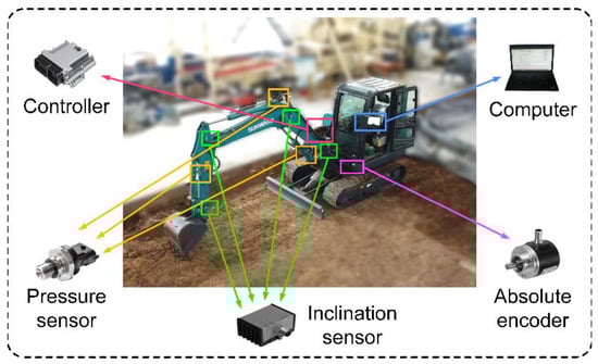
Figure 1.
Overview of the hardware setting.
- A method of finding topologically equivalent waypoints around the teaching excavation motion of a skilled operator;
- A spline-based trajectory optimization framework for generating optimal time-jerk optimality and satisfying kinodynamic feasibility;
- The sensing system, trajectory generation framework and control model are integrated into the autonomous excavator platform, and the aggressive excavation motion is presented in a field test.
The rest of the paper is organized as follows: Section 2 reviews related literature works. The modeling of the system and the trajectory optimization approach are detailed in Section 3 and Section 4, respectively. Section 5 presents the experimental results of the optimal motion generated using our method with the manual excavation motion performed by a skilled operator. Our conclusion and future work are summarized in Section 6.
2. Related Work
There are currently two directions for realizing the motion/trajectory planning of autonomous excavators. One is to model the excavation process based on the skills of skilled operators, then generate some rules that can be used as commands to control autonomous excavation. The other is to generate an optimal motion under dynamic constraints or physical constraints. Here, this paper overviews representative works that are especially relevant to the motion planning of autonomous excavators.
Previous studies have compared some differences in skill between skilled operators and unskilled operators when excavating with regard to specific tasks [6,7]. Some rules for autonomous excavation were extracted via analysis of angle changes in the working device (i.e., swing, boom, stick and bucket). Further, Yamaguchi and Yamamoto [12] transformed these rules into commands to precisely track the excavation motion of skilled operators [13]. Koiwai et al. [14] proposed a method for evaluating and quantifying skills in manual excavation by correlating the performance of different operators and the variations in PID controller parameters. Sekizuka et al. [15] analyzed some geometric indicators (e.g., length of bucket trajectory) of the excavation trajectory through statistical analysis of specific tasks to assess operation skills. Du et al. [2,16] investigated the excavation strategies of expert human operators and their decision-making processes. Then they summarized some rules for when the excavator changed from one stage to the next stage (i.e., bucket fill, bucket lift, swing to dumping, dumping and swing to trench) based on the variation of the joint angle (i.e., swing, boom, stick and bucket) and the trajectory of the bucket teeth [2]. Finally, these were integrated into virtual operator models to control the excavator to complete the trench task.
The above methods provide a way to convert the skills of skilled operators into some rules that can be used to find an excavation path for a specific task. However, the generated trajectory via these methods is generally not the optimal motion; thus, the machine is unable to carry out excavation work quickly and efficiently. Yoo et al. [17] proposed a trajectory optimization method of minimum torque by parametrically representing the trajectory using a B-spline and solving for the optimal trajectory under the maximum flow constraint of the cylinder. Based on previous work [17], Kim et al. [9] obtained the minimum torque trajectory with the constraints of the soil-tool interaction dynamics. Zou et al. [18] formulated a trajectory optimization problem of minimum time, minimum energy consumption and minimum machine damage, which obtained the excavation trajectory under constraints such as kinematics and cylinder maximum pressure. Guan et al. [19] proposed an optimal time trajectory generation method that used NURBS to parameterize the trajectory to generate optimal trajectories that satisfied dynamic constraints. A method using the 4-3-3-3-4 polynomial, which can generate a time-optimal trajectory under the velocity and acceleration constraints, was proposed [20]; however, this method reduced numerical computation efficiency and numerical stability. After that, Zhang et al. [8] adopted cubic splines to represent the excavation trajectory and obtained a time-jerk optimal trajectory. Yang et al. [10] proposed a trajectory optimization framework for a specific excavation task, using a mixed-order spline (5-3-5 polynomial) as an interpolating spline to generate a trajectory under a swept volume and bucket instantaneous direction; they further developed a minimal torque trajectory considering the soil-tool interaction [21]. In addition, MPC (model predictive control) [22] was also used to track the optimal trajectory. Lee et al. [23] used a global planner to generate a reference trajectory that satisfied the maximum bucket volume and minimum force cost, then applied a local planner based on model predictive control to track the reference trajectory. A planning method based on DMP (dynamic movement primitives) that effectively emulated the strategies of experts was developed by Son et al. [24]. However, since these methods cannot explicitly consider constraints (e.g., kinodynamic constraints), the violation of machine physics constraints can occur. At present, there are some new platforms of the trajectory planning of autonomous excavation, such as walking excavators [25,26,27].
Although there are various trajectory planning methods for autonomous excavators in the previous literature, a complete framework has not yet emerged to complete the manual excavation modeling of a skilled operator while incorporating optimal time and smooth trajectory. The strong need for such a framework stems from the fact that high-quality motion requires a combination of skilled operators’ decision making on excavation tasks under changing working conditions. To address this gap, this paper draws on the ideas from [8,10,13] to propose a framework specialized for excavators, exploring and exploiting the excavation skills of skilled operators and trajectory generation.
3. Manual Excavation Model
3.1. System Architecture
The hardware setting of the system is shown in Figure 1. The autonomous excavator is equipped with four inclination sensors and an absolute encoder to measure the angle of the working device (boom, bucket, and stick) and the swing. Three pairs of pressure sensors are used to monitor the pressure in the hydraulic cylinders (boom, stick and bucket) of the work equipment. Computers are used for processing feedback signals of the controller, monitoring pressure changes of cylinders and generating the optimal excavation trajectory. The controller is used to control the electro-hydraulic proportional valve and transmit the sensor signal to the computer.
The overall software architecture of our system is shown in Figure 2. The trajectory execution module was run on a controller, while others were run on the computer. Before the excavation, waypoints were generated according to the topological information of the manual excavation trajectory, and then a reference optimal trajectory was generated within machine kinodynamic constraints. During the excavation, the sensor measured the angle of the working device in real time. Then, the state measurement module preprocessed the data in real time and monitored the pressure changes of the working device. Finally, we used a feedback controller to track the optimal trajectory in real time.
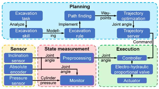
Figure 2.
The architecture of the software system.
3.2. Excavator Kinematics
The generation of the optimal excavation trajectory was generally conducted in the joint space and was utilized to represent the joint angle of the swing, boom, arm and bucket in the joint space. However, the path planning was conducted in the pose space (i.e., task space) according to the excavation task, that is, planned according to the pose of the bucket tooth tip; it was therefore necessary to establish a kinematic model from the joint space to the pose space. Figure 3 shows the Denavit–Hartenberg coordinate system (D–H coordinate system) [28] of the autonomous excavator. The bucket teeth pose is calculated as:
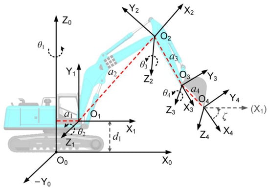
Figure 3.
D–H coordinate system of the autonomous excavator. The red dotted line represents the distance from the intersection of Z0 and Z1 axes to the origin of the O1 coordinate system along Z1, and a2–a4 represent the link lengths of boom, stick, and bucket, respectively.
3.3. Manual Excavation Modeling and Waypoint Finding
3.3.1. Manual Excavation Modeling
To obtain topological information on the excavation path of the skilled operator and find the waypoints, we established the excavation rules of the skilled operator for the trench task (trapezoidal trench). Figure 4 shows a diagram of the bucket teeth path for the five stages for trenching. For trench excavation, the complete operation process can be divided into five stages: bucket penetration, bucket dragging, bucket lifting, swinging to the dumping location and swinging to the trenching location [2].
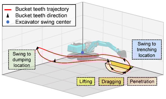
Figure 4.
Illustration of bucket teeth path (red solid line). The black arrows represent bucket teeth orientation. The yellow trapezoid represents the trench. The blue solid dot represents the excavator swing center. The dashed rectangular blocks represent the five excavation stages.
The excavation rules were extracted from the trajectory generated by a skilled operator with more than 10 years of excavation experience. In the stage of penetration, the initial position of the bucket was selected as the position where the bucket was easy to move to the penetration point, and the initial orientation of the bucket was a direction with less soil cutting resistance (the orientation between bucket teeth and ground is about 30° to 60°). In the stage of bucket dragging, the bucket was kept full of soil and horizontal dragging was quickly completed. Third, in the bucket lifting stage, after the second step was completed, the bucket was lifted and rotated to keep the excavated material from falling out of the bucket. During the swing to the dumping location, the bucket pose was kept unchanged and quickly swung to the dumping location (the rotation was set to 90° counterclockwise), slowing down as needed when approaching the dumping location. During the swing to the trenching location, the working device maintained the pose of the previous stage; it adjusted to the pose when approaching the initial penetration location.
3.3.2. Waypoint Finding
After the trajectories of the skilled operators were generated based on the excavation rules, we analyzed the topological information of the trajectory in the joint space. As shown in Figure 5, firstly, the data was processed with the signal alignment method [29] to keep the data length consistent, because operators could not guarantee that the operation state of all tests was completely consistent during the operation. Then, a moving average filter was used to reduce the noise generated by the jerk of the cylinders during excavation. The use of a moving average filter can reduce the interference of noise on the excavator trajectory. Finally, the paths of skilled operators were averaged to obtain a statistically average excavation path [15].
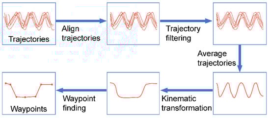
Figure 5.
Diagram of skilled operator’s excavation trajectory analysis and waypoint finding progress.
Since waypoint finding needed to be conducted in the pose space, we needed to transform the obtained joint space trajectory into the pose space. In addition, the excavation path obtained by the skilled operator was extremely poor, as its geometric shape and time distributions were far from optimal. Thus, they were useless or even harmful for trajectory optimization. However, the topological information of the manual excavation paths was essential as it reflected the skilled operator’s intention (e.g., fast and stable excavation). To preserve the topological information of the path and improve the efficiency and quality of the trajectory optimization, this paper proposes an intelligent waypoint selection strategy to obtain a sparse excavation path, these waypoints providing a large degree of freedom for trajectory optimization. The waypoint selection policy borrows an idea from the Douglas–Peucker algorithm [30]. Once all the waypoints are found, these can be used to generate an optimal trajectory that satisfies the dynamic feasibility.
4. Spline-Based Trajectory Optimization
4.1. Problem Formulation
Through the method in Section 3, the topological structure (i.e., waypoints) of the excavation path was obtained. However, optimal trajectories could not be tracked by the controller without trajectory smoothing and time optimization. Therefore, we used a piecewise polynomial to connect these waypoints and formulate a trajectory optimization problem that satisfied kinodynamic feasibility.
The trajectory consisting of piecewise polynomials is parameterized by the time variable in each joint space. The -segment degree polynomial trajectory of the th joint can generally be expressed in the following form:
where is the th segment polynomial coefficient vector and is the time vector.
Excavation is always expected to be as fast as possible, however, this leads to a final state of excavation that is kinodynamically infeasible (i.e., exceeding velocity or acceleration limits), such that the acceleration at the final point is not zero, resulting in a jerk of the mechanical devices. Therefore, we chose the objective function as a trade-off between minimizing the third-order derivative (i.e., jerk) and minimizing time. The general trajectory optimization problem was formulated as:
where is the weight of time; , and are the initial position, velocity and acceleration, respectively; , and are the final position, velocity and acceleration, respectively; and and are the kinodynamic limits.
4.2. Spline Parameterization of Excavation Trajectory
Trajectory optimization problems are usually nontrivial due to the nonlinear constraints in Equation (3), so we needed to make some reasonable choices to make the problem solvable [31]. In this research, the joint trajectories of the excavator manipulator were obtained by using a cubic spline to sequentially pass through the waypoints [32].
For the th joint, is a cubic spline in the interval ; thus, if is a linear function in and is the time interval, then can be written as:
By integrating Equation (4) twice, and by setting and , can be obtained:
Differentiating Equation (5), the and can be expressed as:
According to Equation (6) and the continuity of velocity , we obtained:
The initial velocity and acceleration are specified, and the final velocity and acceleration are also specified values. In addition, two virtual points are set at the second and penultimate positions, respectively [28], giving enough freedom for solving the optimization problem while considering the continuity of velocity and acceleration. Consequently:
Now, the following equation can be concluded from Equations (6)–(8):
where , , are detailed in Appendix A.
To obtain the optimal time and smooth trajectory, the objective function was parameterized using a cubic spline.
A. Object function
where is the number of joints, is the total excavation time, is the weight of time, is the weight of jerk, increasing will cause an aggressive trajectory and is the elastic coefficient, which was introduced to balance this difference between time and jerk, as jerk and time usually have a huge difference in the order of magnitude that results in the role of the time being weakened.
Since the jerk is a constant value in each time interval, substituting Equation (7) into Equation (12) yields the following equation:
B. Velocity constraints:
The velocity is a quadratic function in the time interval ; the maximum absolute velocity exits at , or . Thus, the velocity constraint can be written as:
where
C. Acceleration constraints:
The acceleration is a linear function in the time interval ; the maximum absolute acceleration exits at or . Thus, the acceleration constraint can be written as:
D. Maximum time constraints
where is the maximum time.
Consequently, the trajectory optimization problem is formulated as:
where .
4.3. Execution of the Algorithm
A. Choice of initial solution
The choice of the initial solution of the iterative solution has a significant impact on the optimization result. An inappropriate choice can affect the final optimization result. Therefore, a reasonable determination of the initial solution is the key to solving nonlinear constrained optimization problems.
For the th joint, the time interval must satisfy:
Therefore, the time interval has a lower bound .
Since the above-mentioned lower bound value does not necessarily satisfy the kinodynamic constraints, then the need is expanded by a factor of (i.e., ) times to satisfy kinodynamic constraints, correspondingly, ; the time interval becomes . If , and are used instead of , and , then the following equations can be obtained:
It can be seen from the above equations that as increases by a factor of times, the joint position remains unchanged, while velocity and acceleration are reduced by factors of and , respectively. Now let:
Then the feasibility adjustment factor is obtained by setting:
Finally, the initial solution of the time interval vector is:
where .
B. Execution of the algorithm
Once the initial solution was determined, Equation (20) was solved by running a nonlinear optimization algorithm through a solver. The procedures for solving the trajectory optimization problem are summarized below:
- Start from the given waypoints, the kinodynamic limits and maximum time of excavation;
- Find a suitable initial solution using Equations (21)–(28);
- Choose the appropriate solver and the corresponding optimization algorithm. In this research, SQP (sequential quadratic programming) [33], which tackles nonlinear programming problems by iteratively and locally approximating the original problem with a sequence of quadratic optimization subproblems, was utilized;
- Put the objective function, Equation (12), and constraints, Equations (14), (18) and (19), into the solver;
- Finally, obtain the solution to the optimization problem and trajectory sequence.
5. Results
In this section, the feasibility of our proposed method was validated by comparing autonomous excavation with manual excavation. First, in this paper we conducted several groups of teaching experiments to obtain the waypoints of manual excavation. Then an optimal trajectory was generated through the proposed method in the previous section. Finally, field tests were performed to test our method.
5.1. Implementation Details
Our trajectory generation experiments were completed on the self-developed SWE50E autonomous working excavator platform (Figure 6). Its D–H parameters are shown in Table 1. Computing resources included a laptop computer, which had a dual-core Intel i5-3210 processor running at 2.50 GHz with 12 GB RAM and a BODAS controller. We set the sampling frequency of the controller to 10 Hz to guarantee the controller worked at a high frequency. In the autonomous test, sensors were used to measure online during excavation. The number of waypoints used for trajectory generation in the experiment was set to 169. The kinodynamic feasibility constraints of the autonomous excavator are shown in Table 2. In the trajectory optimization, the maximum number of iterations was set as 50; the time weight and jerk weight were 0.95 and 0.05, which meant that we expected to complete the excavation work as fast as possible; and the elastic coefficient was 0.001. In addition, the maximum time in the excavation process was 90 s.
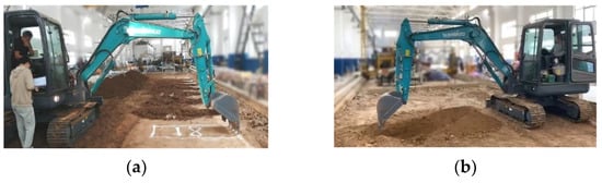
Figure 6.
Scene of manual excavation and autonomous excavation. The number in figure represents the engine speed sets at 1800 rpm. (a) Manual excavation; (b) Autonomous excavation.

Table 1.
D–H parameters of SWE50 excavator.
Table 2.
Kinodynamic feasibility constraints of the excavator.
5.2. Field Test
In this research, the proposed method was tested on a 5-ton autonomous excavator platform. For a fair comparison with a skilled operator (Figure 6), the size of the trench was set as 2 × 0.8 × 1 m and the engine speed of excavator was set as 1800 rpm for the test. The distance between the farthest edge of the excavation area and the crawler was 3.5 m. During the dumping stage, the body rotated 90° counterclockwise. As shown in Figure 7a, for an operation cycle that included seven shovels of excavation, the operation time was as consistent as possible. First, the excavator performed 15 operation cycles (note that it required fast and smooth excavation trajectories) and recorded the excavation trajectories of a skilled operator. Then, the waypoints were obtained through the method in Section 3. Finally, the excavation trajectory was generated using the method in Section 4. It should be noted that this paper focuses on the specified dimension of the trench. Afterwards, the autonomous excavation was completed by controlling the excavator arm (i.e., boom, stick and bucket) to track the generated trajectory. To compare angle and pressure, this paper only compares the joint angle of the excavator working devices (i.e., this trajectory is YZ projection as shown in Figure 7b) and the corresponding cylinder pressure (boom, stick, bucket) (Figure 8 and Figure 9).
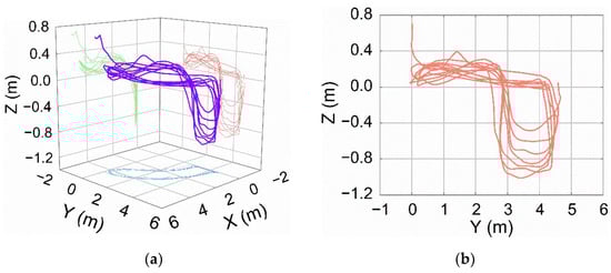
Figure 7.
Bucket-tip trajectory in pose space according to our proposed method. Purple, blue, green and red curves are optimal trajectory, XY projection, XZ projection and YZ projection, respectively. (a) Optimal trajectory; (b) YZ projection of optimal trajectory.
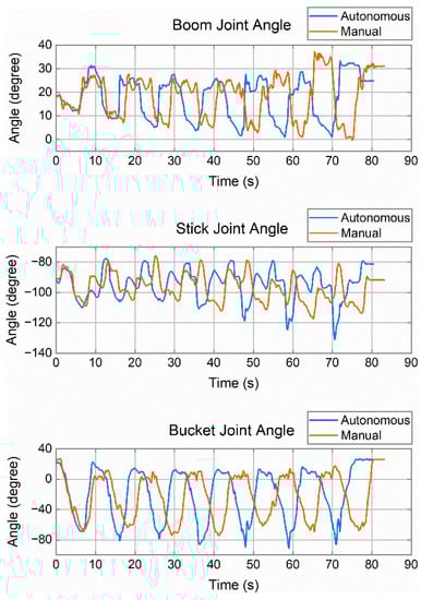
Figure 8.
A comparison of joint trajectory between autonomous and manual excavation. The blue curve is autonomous excavation and the red curve is manual excavation.
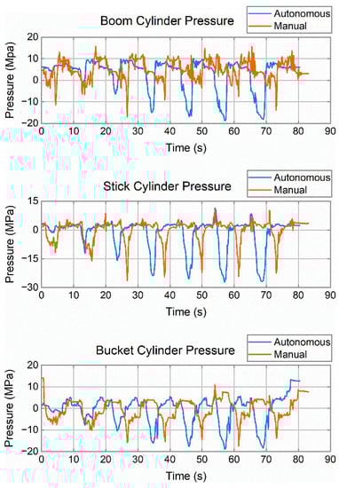
Figure 9.
A comparison of autonomous and manual excavation cylinder pressure. The blue curve is autonomous excavation and the red curve is manual excavation.
By comparing the autonomous excavation trajectory using the proposed method with the excavation trajectory of a skilled operator, as shown in Figure 8, we see that the method of this paper presents a shorter time while satisfying the dynamic feasibility constraints. In the experiment, the time of autonomous excavation was 80.4 s, while that of the operator was 83.2 s, as listed in Table 3. By using this method proposed, the speed and acceleration during the excavation motion are closer to the dynamic feasibility limit; hence, autonomous excavation tends to move faster. However, it can be seen that the angle fluctuation of each joint in autonomous excavation (comparison of standard deviation in Table 3) is larger when compared with that of manual excavation.
Table 3.
Comparison of autonomous and manual excavation joint motion.
On the other hand, as shown in Figure 9, the maximum absolute pressure of the working device was larger than that of manual excavation, due to the aggressiveness of the excavator being fully used. However, this led to a larger standard deviation of the pressure of the working device for autonomous excavation motion (as shown in Table 4); this is because a large jerk of the cylinder results in unstable motion during the operation, and the stability of the movement is therefore worse than manual operation.
Table 4.
Comparison of manual and autonomous excavation cylinder pressure.
For a fair comparison, we compared the proposed method against the previous excavation trajectory generation research based on optimization and bucket capacity [8,19]. In the case of an average excavation cycle, the time used in this paper was 11.5 s with a bucket capacity of 0.18 m3, while the previous research [19] presented 14.59 s with a bucket capacity of 0.02 m3. Additionally, the difference in excavation efficiency is that this paper considered the dynamic feasibility limit of the actuators, thereby making full use of the physical properties of the excavator itself, while the previous research only considered a single time constraint, this leading to the difference in excavation time between the two. In turn, smoother excavation trajectories also promoted better time optimization.
6. Conclusions
In this paper, a novel trajectory generation method is proposed for autonomous excavator teach-and-plan. Detailed conclusions are the following:
- In this paper, the waypoints used for optimal trajectory generation were obtained by combining a manual excavation model with trajectory topology information using the excavation trajectories of skilled operators;
- These waypoints were iteratively optimized in a nonlinear optimization framework to generate fast, smooth and efficient excavation motions while satisfying kinodynamic feasibility constraints;
- A comparison experiment between autonomous excavation and manual excavation highlights the superiority of this method in aggressiveness.
In this work, we assumed that the excavation environment was relatively static (e.g., no earthwork collapses) and that the autonomous excavator was instructed to track the reference trajectory once it was generated. In future research, we will focus on the following aspects:
- To add reactive local replanning to the current framework to handle a dynamic excavation environment. In this way, the generated repetitive trajectory will be used as a reference trajectory for the autonomous excavator. Then, the autonomous excavator will track the reference trajectory and avoid the problem of changes in trench size through local trajectory planning;
- Combine the excavation volume constraint, and transform it into a constraint of the trajectory optimization problem. Then, a full excavation bucket will be achieved.
Author Contributions
Conceptualization, J.Z., Y.H. and M.T.; methodology, J.Z., C.L. and X.X.; software, J.Z. and C.L.; validation, J.Z. and C.L.; formal analysis, J.Z. and X.X.; data curation, J.Z.; writing—original draft preparation, J.Z.; writing—review and editing, J.Z., M.T. and X.X.; supervision, Y.H., M.T. and X.X.; project administration, Y.H. and M.T.; funding acquisition, Y.H. All authors have read and agreed to the published version of the manuscript.
Funding
This research was funded by the Fundamental Research Funds for the Central Universities of Chang’an University, grant number 300102259503.
Institutional Review Board Statement
Not applicable.
Informed Consent Statement
Not applicable.
Data Availability Statement
Not applicable.
Acknowledgments
The authors are gratefully thankful for the support by the Fundamental Research Funds for the Central Universities of Chang’an University. The authors also thank graduate researchers Zhiqiang Wang, Chaofan Li, Yujie Hou, Peng Tan, Fanwei Meng and Hao Huang for their assistance in this research.
Conflicts of Interest
The authors declare no conflict of interest.
Appendix A
Given the initial and final velocity and acceleration are both zero, and the continuity of acceleration:
It can be obtained from Equations (6)–(8) and (A1):
Hence, a linear equation is obtained, which can be written as:
where
and
References
- Melenbrink, N.; Werfel, J.; Menges, A. On-site autonomous construction robots: Towards unsupervised building. Autom. Constr. 2020, 119, 103312. [Google Scholar] [CrossRef]
- Du, Y.; Dorneich, M.C.; Steward, B. Virtual operator modeling method for excavator trenching. Autom. Constr. 2016, 70, 14–25. [Google Scholar] [CrossRef][Green Version]
- Sing, S. Synthesis of Tactical Plans for Robotic Excavation; Carnegie Mellon University: Pittsburgh, PA, USA, 1995. [Google Scholar]
- Bradley, D.A.; Seward, D.W. Developing real-time autonomous excavation-the LUCIE story. In Proceedings of the 1995 34th IEEE Conference on Decision and Control, New Orleans, LA, USA, 13–15 December 1995; pp. 3028–3033. [Google Scholar]
- Stentz, A.; Bares, J.; Singh, S.; Rowe, P. A robotic excavator for autonomous truck loading. Auton. Robot. 1999, 7, 175–186. [Google Scholar] [CrossRef]
- Sakaida, Y.; Chugo, D.; Kawabata, K.; Kaetsu, H.; Asama, H. The analysis of excavator operation by skillful operator. In Proceedings of the 23rd International Symposium on Automation and Robotics in Construction, Tokyo, Japan, 3–5 October 2006; pp. 543–547. [Google Scholar]
- Sakaida, Y.; Chugo, D.; Yamamoto, H.; Asama, H. The analysis of excavator operation by skillful operator-extraction of common skills-. In Proceedings of the 2008 SICE Annual Conference, Chofu, Japan, 20–22 August 2008; pp. 538–542. [Google Scholar]
- Zhang, Y.; Sun, Z.; Sun, Q.; Wang, Y.; Li, X.; Yang, J. Time-jerk optimal trajectory planning of hydraulic robotic excavator. Adv. Mech. Eng. 2021, 13, 16878140211034611. [Google Scholar] [CrossRef]
- Kim, Y.B.; Ha, J.; Kang, H.; Kim, P.Y.; Park, J.; Park, F.C. Dynamically optimal trajectories for earthmoving excavators. Autom. Constr. 2013, 35, 568–578. [Google Scholar] [CrossRef]
- Yang, Y.; Long, P.; Song, X.; Pan, J.; Zhang, L. Optimization-based framework for excavation trajectory generation. IEEE Robot. Autom. Lett. 2021, 6, 1479–1486. [Google Scholar] [CrossRef]
- Gao, F.; Wang, L.; Wang, K.; Wu, W.; Zhou, B.; Han, L.; Shen, S. Optimal trajectory generation for quadrotor teach-and-repeat. IEEE Robot. Autom. Lett. 2019, 4, 1493–1500. [Google Scholar] [CrossRef]
- Yamaguchi, T.; Yamamoto, H. Motion analysis of hydraulic excavator in excavating and loading work for autonomous control. In Proceedings of the 23rd International Symposium on Automation and Robotics in Construction, Tokyo, Japan, 3–5 October 2006; pp. 602–607. [Google Scholar]
- Shao, H.; Yamamoto, H.; Sakaida, Y.; Yamaguchi, T.; Yanagisawa, Y.; Nozue, A. Automatic excavation planning of hydraulic excavator. In Proceedings of the International Conference on Intelligent Robotics and Applications, Wuhan, China, 15–17 October 2008; pp. 1201–1211. [Google Scholar]
- Koiwai, K.; Yamamoto, T.; Nanjo, T.; Yamazaki, Y.; Fujimoto, Y. Data-driven human skill evaluation for excavator operation. In Proceedings of the 2016 IEEE International Conference on Advanced Intelligent Mechatronics (AIM), Banff, AB, Canada, 12–15 July 2016; pp. 482–487. [Google Scholar]
- Sekizuka, R.; Ito, M.; Saiki, S.; Yamazaki, Y.; Kurita, Y. Evaluation system for hydraulic excavator operation skill using remote controlled excavator and virtual reality. In Proceedings of the 2019 IEEE/RSJ International Conference on Intelligent Robots and Systems (IROS), Macau, China, 3–8 November 2019; pp. 3229–3234. [Google Scholar]
- Du, Y.; Dorneich, M.C.; Steward, B. Modeling expertise and adaptability in virtual operator models. Autom. Constr. 2018, 90, 223–234. [Google Scholar] [CrossRef]
- Yoo, S.; Park, C.-G.; You, S.-H.; Lim, B. A dynamics-based optimal trajectory generation for controlling an automated excavator. Proc. Inst. Mech. Eng. Part C J. Mech. Eng. Sci. 2010, 224, 2109–2119. [Google Scholar] [CrossRef]
- Zou, Z.; Chen, J.; Pang, X. Task space-based dynamic trajectory planning for digging process of a hydraulic excavator with the integration of soil–bucket interaction. Proc. Inst. Mech. Eng. Part K J. Multi-Body Dyn. 2019, 233, 598–616. [Google Scholar] [CrossRef]
- Guan, C.; Wang, F.; Zhang, D.-y. NURBS-based time-optimal trajectory planning on robotic excavators. J. Jilin Univ. (Eng. Technol. Ed.) 2015, 45, 540–546. [Google Scholar] [CrossRef]
- Sun, Z.; Zhang, Y.; Li, H.; Sun, Q.; Wang, Y. Time optimal trajectory planning of excavator. J. Mech. Eng. 2019, 55, 166–174. [Google Scholar] [CrossRef]
- Yang, Y.; Pan, J.; Long, P.; Song, X.; Zhang, L. Time variable minimum torque trajectory optimization for autonomous excavator. arXiv 2020, arXiv:2006.00811. [Google Scholar] [CrossRef]
- Wind, H.; Renner, A.; Bender, F.A.; Sawodny, O. Trajectory generation for a hydraulic mini excavator using nonlinear model predictive control. In Proceedings of the 2020 IEEE International Conference on Industrial Technology (ICIT), Buenos Aires, Argentina, 26–28 February 2020; pp. 107–112. [Google Scholar]
- Lee, D.; Jang, I.; Byun, J.; Seo, H.; Kim, H.J. Real-time motion planning of a hydraulic excavator using trajectory optimization and model predictive control. In Proceedings of the 2021 IEEE/RSJ International Conference on Intelligent Robots and Systems (IROS), Prague, Czech Republic, 27 September–1 October 2021; pp. 2135–2142. [Google Scholar]
- Son, B.; Kim, C.; Kim, C.; Lee, D. Expert-emulating excavation trajectory planning for autonomous robotic industrial excavator. In Proceedings of the 2020 IEEE/RSJ International Conference on Intelligent Robots and Systems (IROS), Las Vegas, NV, USA, 24 October–24 January 2021; pp. 2656–2662. [Google Scholar]
- Jud, D.; Hottiger, G.; Leemann, P.; Hutter, M. Planning and control for autonomous excavation. IEEE Robot. Autom. Lett. 2017, 2, 2151–2158. [Google Scholar] [CrossRef]
- Jud, D.; Leemann, P.; Kerscher, S.; Hutter, M. Autonomous free-form trenching using a walking excavator. IEEE Robot. Autom. Lett. 2019, 4, 3208–3215. [Google Scholar] [CrossRef]
- Jelavic, E.; Berdou, Y.; Jud, D.; Kerscher, S.; Hutter, M. Terrain-adaptive planning and control of complex motions for walking excavators. In Proceedings of the 2020 IEEE/RSJ International Conference on Intelligent Robots and Systems (IROS), Las Vegas, NV, USA, 24 October–24 January 2021; pp. 2684–2691. [Google Scholar]
- Siciliano, B.; Sciavicco, L.; Villani, L.; Oriolo, G. Robotics: Modelling, Planning and Control, 1st ed.; Springer: London, UK, 2009; p. 632. [Google Scholar] [CrossRef]
- Proakis, J.G.; Manolakis, D.G. Digital Signal Processing: Principles Algorithms and Applications, 4th ed.; Prentice-Hall, Inc.: Upper Saddle River, NJ, USA, 2007; p. 1104. [Google Scholar]
- Douglas, D.H.; Peucker, T.K. Algorithms for the reduction of the number of points required to represent a digitized line or its caricature. Cartogr.Int. J. Geogr. Inf. Geovisualization 1973, 10, 112–122. [Google Scholar] [CrossRef]
- Lin, C.; Chang, P.; Luh, J. Formulation and optimization of cubic polynomial joint trajectories for industrial robots. IEEE Trans. Autom. Control 1983, 28, 1066–1074. [Google Scholar] [CrossRef]
- Gasparetto, A.; Zanotto, V. A technique for time-jerk optimal planning of robot trajectories. Robot. Comput. Integr. Manuf. 2008, 24, 415–426. [Google Scholar] [CrossRef]
- Nocedal, J.; Wright, S.J. Numerical Optimization, 2nd ed.; Springer: New York, NY, USA, 2006; p. 664. [Google Scholar] [CrossRef]


Publisher’s Note: MDPI stays neutral with regard to jurisdictional claims in published maps and institutional affiliations. |
© 2022 by the authors. Licensee MDPI, Basel, Switzerland. This article is an open access article distributed under the terms and conditions of the Creative Commons Attribution (CC BY) license (https://creativecommons.org/licenses/by/4.0/).