Polygonal Wear Mechanism of High-Speed Train Wheels Based on Lateral Friction Self-Excited Vibration

Abstract

This work details research on the formation mechanism of wheel polygonalization in high-speed trains and its effect factors by numerical modeling in order to prevent the increasingly prevalent problem of wheel polygonal wear. The lateral self-excited vibration model of a wheel was developed using the LuGre friction model and self-excited vibration theory. The properties of wheel self-excited vibration and the crucial condition of Hopf bifurcation were investigated; the process of wheel polygonal wear was simulated and the results were validated using field tracking data. The results demonstrated that periodic self-excited vibration generated by Hopf bifurcation is a required condition for polygonal wheel attrition at a given speed. The wheel’s polygonal wear has the following characteristics: “Constant speed—Self-excited—Fixed frequency—Divisible.” The order of the polygon is determined by the ratio of the wheel lateral self-excited vibration frequency to its rotational frequency. Wheel polygonal wear was caused by the vertical dynamic force of the wheel rail. The findings of the study can serve as a theoretical foundation for the prediction and reduction of wheel polygonal wear.

1. Introduction

Wheel polygonalization, particularly high-order polygonalization, is becoming increasingly popular. This not only causes premature wheel scrapping, but also damages or causes failure of vehicle and track components, jeopardizing operational safety [1,2]. Wang, et al. [3] undertook field tracking experiments of high-speed EMUs from various railway lines, operating speeds, and train models, and found that wheelbase, fastener type, and ambient temperature are all strongly connected to polygonal wear. Tao, et al. [4] studied the polygonal wear characteristics of Chinese mainstream electric locomotive wheels. They discovered the process of polygonal wear generation and major influencing elements, and the influence of wheel re-profiling on the wheel polygon was also researched and addressed. Wu, et al. [5] conducted extensive field tests to examine the process of high-order polygonal wear on high-speed wheels. It was discovered that altering the running speed significantly prevented polygonal wear. Nielsen and Johansson [6] investigated the categorization, fundamental causes, and effects of abnormalities in long-wavelength wheel tread. Johansson, et al. [7] modelled the evolution of wheel polygonal wear and discovered that vertical track anti-resonance and P2resonance at 165 Hz were the sources of polygonal wear. Morys [8] discovered that the third-order initial polygonal wear arouses the first-order bending vibration of the wheelset, generating lateral creep and increasing the development of polygonal wear.

Chen, et al. [9] postulated that self-excited friction vibration of a wheel–rail system generates polygonal wear in 2011, and projected comparable consequences to that of a high-speed train. Zhao, et al. [10] investigated the features of wheel–rail self-excited vibration, as well as the mechanism and affecting variables of polygonal wheel wear. They claimed that polygonation was easily induced by friction self-excited vibration caused by saturation of wheel–rail creep force on a straight path. Cui, et al. [11] studied the dynamic cause of rail corrugation by the theories of self-excitation. Wu, et al. [12] investigated the effect of disc brake units on the polygonal wear generation of high-speed railway wheels by friction self-excited vibration. However, whether the condition of self-excited friction vibration can be accomplished in operation, and whether the wear would appear polygon after the self-excited friction vibration, has yet to be examined and validated.

The circumstances of polygonal wear of wheels were examined in this research using the wear work model, and the calculation equation of polygonal wear order of wheels was provided. The stability of wheel self-excited vibration was investigated using a dynamic model of wheel lateral self-excited vibration based on the LuGre friction model. The properties of wheel polygonal wear were discovered, and field data were validated. This establishes a theoretical foundation for comprehending the mechanics of polygonal wear.

2. Conditions of Polygonal Wear

2.1. Model of Wheel Circumference Wear Depth

Archard and wear work models of wheel material wear are examples. The study found that the wheel polygon development tendency of the two models is almost identical; however, the Archard model has a higher wear coefficient. The results of the wear work model are more accurate, and the computation efficiency is greater [13,14]. As a result, the wear work model is used for simulation analysis in this research. The wear mass Δm is proportional to the wear work W_w, according to the following model:

$$\begin{array}{l}\Delta m=K_w\cdot W_w\\ =K_w\cdot {\displaystyle \int P_w}\mathrm{d}t=K_w\cdot {\displaystyle \iint \tau \cdot s\mathrm{d}A\mathrm{d}t}\end{array}$$

(1)

where, K_w and P_w are the wear work coefficient and wear power, respectively, and τ, s, and A are the lateral stress in the contact spot element, the creep speed, the contact spot area, respectively.

Assuming θ is a point of the circumference of wheel rolling, the radius is R(θ) and the radius of the last turn of the wheel is R(θ − 2π). The wear depth Δr = R(θ − 2π) − R(θ). In addition, the wear mass is the product of the wear depth, contact spot area, and material density, that is, Δm = ρAΔr.

The wear depth results of the global technique and the local method for the contact model concur well. However, the latter’s calculation speed is double that of the former [15]. As a result, this research employs a global technique to investigate the contact parameters on the whole wheel–rail contact region, focusing on the average value of normal force, tangential force, and relative velocity. The tangential force and slip velocity of each element at the contact site are considered to have identical tangential stress τ_e and slip velocity s_e. Combining Equation (1) and r(θ) yields the equation for determining wear depth Δr(θ).

$$\begin{array}{l}\Delta r(\theta )=\frac{\Delta m}{\rho A}=K_w\cdot W_w=K_w\cdot {\displaystyle \iint \frac{\tau \cdot s}{\rho A}\mathrm{d}A\mathrm{d}t}=K_w\cdot \frac{({\tau }_{e}A)\cdot L_e}{\rho b\cdot L_e}\\ =K_w\cdot \frac{F_{\tau }}{\rho b}\end{array}$$

(2)

where Fτ is tangential creep force, ρ is density of wheel material, and b is average width of the wear zone.

The remaining radius of the wheel circle θ is

$$R(\theta )=R(\theta -2\pi )-\Delta r(\theta )$$

(3)

2.2. The Conditiom of Polygonal Wear

According to Equation (2), wheel wear is proportional to the tangential creep force. When the tangential creep force changes at a given frequency, the wear depth changes as well, resulting in wheel polygonation. The peak of wear happens just once in a tangential vibration cycle when the tangential creep force reaches its maximum.

The time interval between two consecutive wear peaks is 1/f₁ if the tangential vibration frequency is f₁. The wheel rotation duration is 1/f₂ if the wheel rotational frequency is f₂. The peak value of wear N within a rolling circle may then be calculated.

$$N=\frac{f_1}{f_2}$$

(4)

while $f_2=V/2\pi R$,

$$f_1=N{f}_2=\frac{NV}{\pi D}$$

(5)

where V is the speed of the train and D is the nominal diameter of the wheel. There are two cases:

(1)

The wear depth at a certain position around the wheel is the same for each wheel rolling circle when the tangential vibration frequency is an approximate integer multiple of the wheel rotational frequency. The wear peak always emerges in certain regions, and the wheel circumference will become polygonal after a long period.

(2)

When the tangential vibration frequency is not an approximate integer multiple of the wheel rotational frequency, and the wear depth at a certain spot around the wheel varies within two rounds of wheel rolling. The last circle’s highest point of wear may wear less. After a long period of operation, the wheel circumference will be consistent, and polygonal wear will not be visible.

According to the preceding study, tangential vibration is simply a required condition for polygonal wear. The ratio of wheel tangential vibration frequency to wheel rotational frequency determines the sequence of wheel polygonal wear. As a result, the tangential vibration condition of the wheel must be analyzed to establish the range of factors that might lead to polygonation.

3. Analysis of Lateral Self-Excited Vibration of Wheel–Rail Contact

Tangential force is also known as creep force, and it is further subdivided into lateral creep force and longitudinal creep force. We already investigated the influence of longitudinal creep force on polygonal wheel wear [16], thus this article focuses solely on the effect of lateral creep.

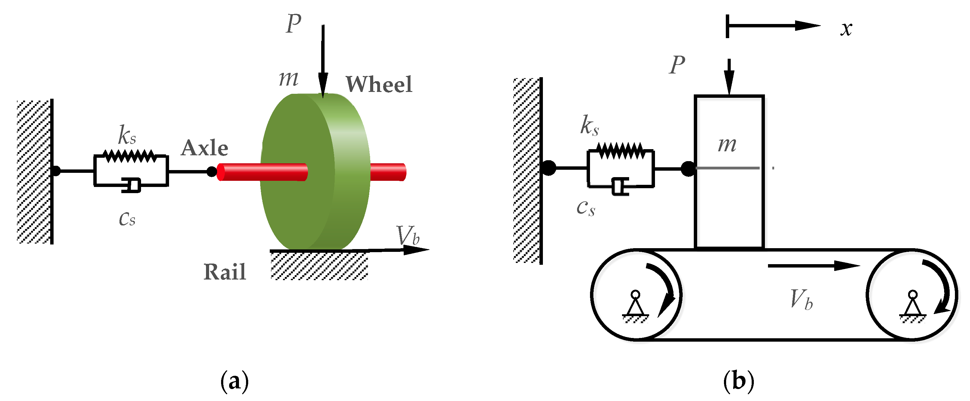
3.1. Model of Lateral Self-Excited Friction Vibration of Wheel

The wheel–rail system connects the sprung mass to the under rail foundation; the vibration of the wheelset and rail subsystem is the primary source of polygonal wheel degradation. As a result, as shown in Figure 1a, the model of wheel–rail lateral self-excited friction is created in this research, using the following assumptions:

(1)

The wheel–rail contact is simplified to cylinder–plane contact by ignoring the slope of the tread and the curvature of the rail.

(2)

Owing to the symmetry of the wheelset and track construction, only half of the wheel–rail subsystem is chosen.

(3)

The axle is considered a massless elastic entity, with the mass centered on the wheel. The symmetrical constraint is placed on the symmetrical surface, and the connection mode of wheel and axle is equivalent to the lateral stiffness damping provided by the flexibility of 1/2 axle and 1 wheel.

(4)

The sprung mass of the vehicle body and the under foundation of the rail are simplified into wheel load P, which includes static load P0 and dynamic load ΔP, and the rail rigidity is assumed to be infinite.

In Figure 1b, m, c_s, and k_s represent the wheel equivalent mass, damping, and stiffness, respectively. V_b is the lateral linear velocity of the wheel relative to the rail surface, and V_b = Vsinψ, where V is the speed and ψ is the rolling angle of the wheelset.

While the lateral movement of the wheel on the rail is as simple as the turn of the belt pulley (as illustrated in Figure 1b), the creep force between the wheel and the rail provides the vibration energy input. Assume that the wheel’s displacement to the original position (i.e., the position of the spring and damper when no force is applied) is x and the creep speed between the wheel and the belt (rail) is as follows:

$$V_r=V\sin \psi -\dot{x}$$

(6)

Then, the lateral vibration equation of the wheel is as follows:

$$m\ddot{x}+c_s\dot{x}+k_{s}x=F_{\tau }$$

(7)

where F_τ is the wheel–rail creep force, and F_τ = μP.

The wheel–rail creep force has a significant impact on the lateral vibration of the wheel–rail. There is a complex nonlinear relationship between the creep coefficient μ and the creep rate [17,18], as shown in Figure 2. When the creep speed is between 0 and 0.37 m/s, the creep coefficient rapidly increases, the creep force is static friction, and the slope of the creep coefficient curve is positive and steep. When the creep speed exceeds 0.37 m/s, the wheel starts to slide, the creep force progressively changes from static to dynamic friction, and the creep coefficient drops as the creep speed increases. The slope of the creep coefficient curve is negative at this point and subsequently declines.

It can be seen that the creep force Fτ is a function of creep speed Vr:

$$F_{\tau }=f(V_r)=f(V\sin \psi -\dot{x})$$

(8)

The creep force is expanded by first-order Taylor at the creep speed:

$$\begin{array}{l}{F}_{\tau }=f(V_{r0})+f^{\prime }(V_{r0})[(V\sin \psi -\dot{x})-V_{r0}]\\ =[f(V_{r0})+f^{\prime }(V_{r0})(V\sin \psi -V_{r0})]-f^{\prime }(V_{r0})\dot{x}\end{array}$$

(9)

Substituting Equation (9) into Equation (7), a vibration equation based on Taylor expansion of creep force is obtained.

$$m\ddot{x}+[c_s+f^{\prime }(V_{r0})]\dot{x}+k_{s}x=0$$

(10)

That is

$$m\ddot{x}+(c_s+c_{fe})\dot{x}+k_{s}x=0$$

(11)

where C_fe is the equivalent damping of creep force and is equal to the slope of the creep speed-creep coefficient curve.

The equation has an approximate solution:

$$x=A{e}^{\alpha t}\sin (\omega t+\varphi )$$

(12)

where A is the constant, ω is circular frequency of the system, $\omega ={\omega }_n\sqrt{1+{\xi }^2},{\omega }_n=\sqrt{k_s/m}$,$\alpha =-(c_s+c_{fe})/m$, damping ratio $\xi =c_s/(2\sqrt{m{k}_s})$, and $\varphi$ is the phase angle.

According to Equation (12), α < 0, under the initial disturbance, the vibration of the wheel will gradually converge to zero. That is, in the positive slope of the creep coefficient- creep speed curve shown in Figure 2, c_s + c_fe > 0, and the wheel tends to be stable.

When α > 0, in the negative slope, and c_s + c_fe < 0. Wheel amplitude increases exponentially with time, and the wheel tends towards unstable dynamic sliding.

When α = 0, c_s + c_fe = 0, the wheel amplitude does not change with time, and the wheel tends towards unstable steady sliding, resulting in the periodic change in lateral creep force Fτ, which leads to polygonal wear of the wheel. The system obviously does not contain external excitation, but the wheel produces self-excited vibration.

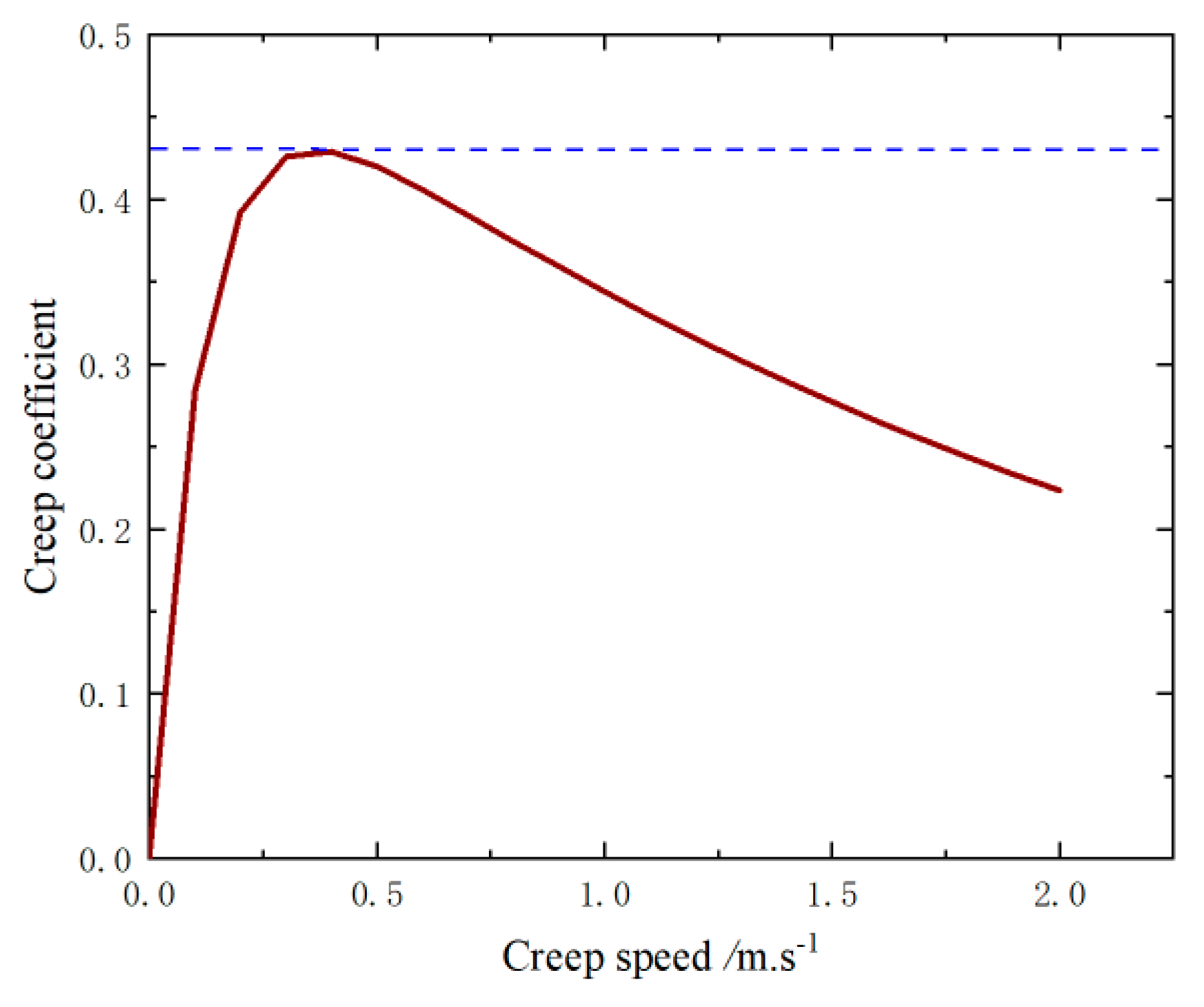
3.2. LuGre Friction Model

The production of self-excited vibration in a wheel–rail system requires a negative slope of the creep coefficient curve. Self-excited vibration causes unstable continuous sliding of the wheel, resulting in polygonal wear. It is critical to correctly duplicate the force transmission between the wheel and the rail in order to examine the self-excited vibration of the wheel. The wheel lateral vibration is mainly dry friction motion, while the LuGre model presented by Canudas, et al. [19] accurately represents the “negative slope” in the friction process and fits the experimental results nicely. As a result, the LuGre model was utilized in this work to represent lateral creep force.

$$\{\begin{array}{l}{F}_{\tau }={\sigma }_0\mathrm{z}+{\sigma }_1\dot{z}+{\sigma }_2{V}_r\\ \dot{z}=V_r-\frac{\left|V_r\right|}{g(V_r)}{\sigma }_{3}z\\ g(V_r)=F_s+(F_m-F_s)e^{-\left|V_r/V_s\right|{}^{\phi }}\end{array}$$

(13)

where σ₀ and σ₁ are the equivalent stiffness and damping coefficient of brush sliding displacement and sliding speed after differential treatment by friction force, respectively. σ₂ is the relative viscous damping coefficient, σ₃ is the wheel–rail contact stiffness, z is the elastic deformation of brush, V_s is the Stribeck speed in steady-state friction characteristics, φ is Stribeck index of steady-state friction, F_m is the maximum static friction force (F_m = μ_mP₀sinψ), F_s is the sliding friction (F_s = μ_sP₀sinψ), μ_m is the maximum static friction coefficient, and μ_s is the dynamic friction coefficient.

The vibration differential equation of the system can be obtained by combining Equations (6), (7), and (13):

$$\{\begin{array}{l}m\ddot{x}+c_s\dot{x}+k_{s}x+{\sigma }_0\mathrm{z}+{\sigma }_1\dot{z}=0\\ \dot{z}=(\dot{x}-V\cdot \sin \psi )-\frac{|\dot{x}-V\cdot \sin \psi |}{F_s+(F_m-F_s)e^{-\left|(\dot{x}-V\cdot \sin \psi )/V_s\right|\phi }}{\sigma }_{0}z\end{array}$$

(14)

The equation describes the process of wheel lateral vibration evolution, and its equilibrium solution corresponds to the system’s stable state. The periodic solution indicates that the system generates self-excited vibration, which could result in wheel polygonation.

3.3. Wheel Rail Vertical Force Model

Sleeper spacing, pits, the initial polygonal of wheel tread, or wheel eccentricity can all cause a periodic change in vertical wheel–rail contact pressure. As a result, the wheel rail vertical force model is as follows:

$$F_z=P_0(1+k_d\sin n_d\omega t)$$

(15)

where P₀ is wheel load and k_d and N_d are the dynamic load coefficient and frequency ratio, respectively.

3.4. The Lateral Stiffness of the Wheel Is Determined

Before solving the above model, the modal mass, stiffness, and damping of the wheel must be determined. These parameters are related to the flexible wheel mode with the highest lateral vibration trend. The wheel is discretized into a vibration system with n concentrated masses, each with one degree of freedom in the U direction.

The motion equation of the system is follows:

$$[M]\{\ddot{U}\}+[C]\{\dot{U}\}+[K]\{U\}=-[M]\{I\}{\ddot{u}}_b(t)$$

(16)

The structural displacement response can be transformed from physical coordinates to modal coordinates within the linear range.

$$\{U\}=[\mathsf{\Phi }]\{q\}={\displaystyle \sum _{i=1}^n\left\{{\varphi }_i\right\}}{q}_i$$

(17)

The unit vector {I}, which represents the rigid body displacement of the system, can also be expressed as the linear superposition of each modal vector {φ_i},

$$\{I\}={\displaystyle \sum _{i=1}^n\left\{{\phi }_i\right\}}{\gamma }_i$$

(18)

where γ_i is the rigid body displacement mode participation factor, which indicates the contribution amount of each restricted mode when the system is not deformed and just follows the foundation rigid body displacement.

The mass matrix [M] and stiffness matrix [K] satisfy the modal orthogonality, and the damping matrix [C] is assumed to also satisfy the modal orthogonality. Then, Equation (16) can be decoupled into n independent equations.

$$M_i{\ddot{q}}_i+C_i{\ddot{q}}_i+K_i{q}_i=-M_i{\gamma }_i{\ddot{u}}_b(t)$$

(19)

where M_i, C_i, and K_i are defined as follows:

$$\begin{array}{l}{M}_i={\left\{{\phi }_i\right\}}^{\mathrm{T}}[M]\{{\phi }_i\}\\ C_i={\left\{{\phi }_i\right\}}^{\mathrm{T}}[C]\{{\phi }_i\}\\ K_i={\left\{{\phi }_i\right\}}^{\mathrm{T}}[K]\{{\phi }_i\}\end{array}$$

(20)

Solve Equation (16) to obtain q_i, and then use Equation (17) to obtain {U}.

The structural modal vector {φ_i} only reflects the ratio of the displacements of each node, which can be multiplied by any constant factor, so the value of γ_i is not fixed. The values of M_i, C_i, and K_i maintain the same proportion relationship, as follows:

$$\begin{array}{l}{K}_i/M_i={\omega }_i^2\\ C_i/M_i=2{\zeta }_i{\omega }_i\end{array}$$

(21)

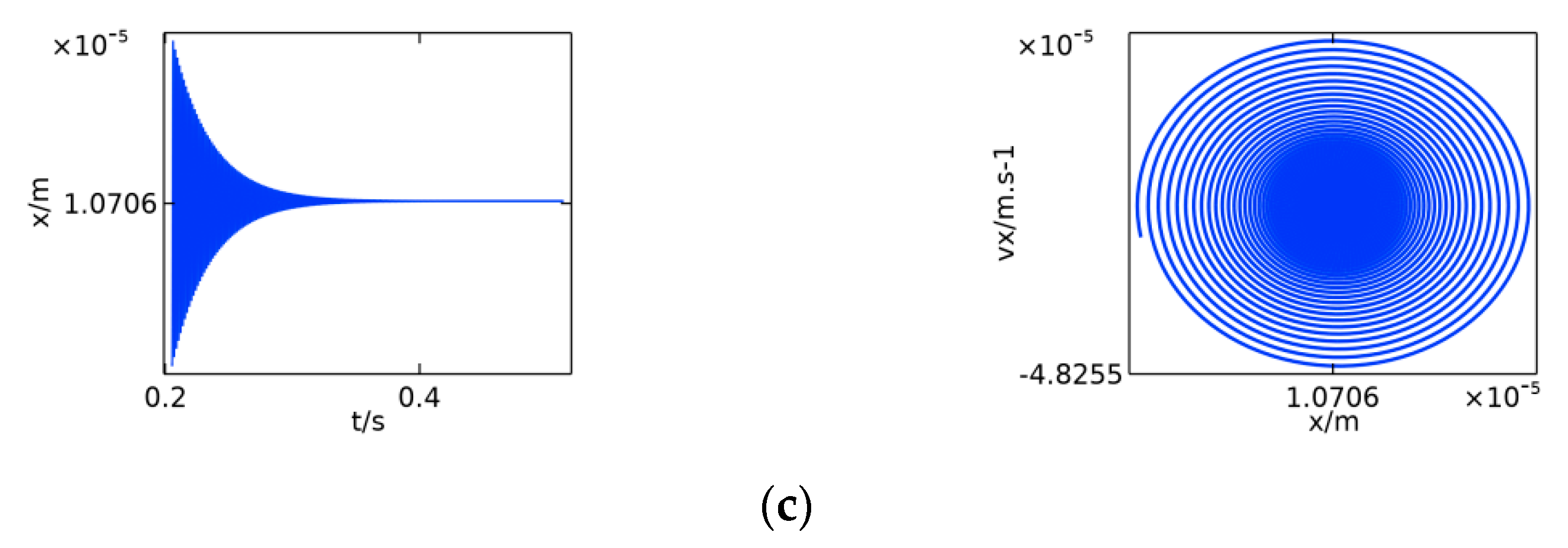
3.5. Analysis of System Stability

Letting x₁ = x and x₃ = z, Equation (14) will be

$$\{\begin{array}{l}{\dot{x}}_1=x_2\\ {\dot{x}}_2=-(c_s{x}_2+k_s{x}_1+{\sigma }_0{x}_3+{\sigma }_1{\dot{x}}_3)/m\\ {\dot{x}}_3=(x_2-V\sin \Psi )-\frac{|x_2-V\sin \Psi |}{F_s+(F_m-F_s)e^{-\left|\right(x_2-V\sin \Psi )/V_s|\varphi }}{\sigma }_0{x}_3\end{array}$$

(22)

Substituting $\dot{ x_1}=\dot{x_2}=\dot{x_3}$ = 0 into Equation (22), the equilibrium point is

$$\{\begin{array}{l}{x}_{10}=-\frac{F_s+(F_m-F_s)e^{-(V\sin \Psi /V_s)}{}^{\varphi }}{k_s}\\ x_{20}=0\\ x_{30}=\frac{F_s+(F_m-F_s)e^{-(V\sin \Psi /V_s)}{}^{\varphi }}{{\sigma }_0}\end{array}$$

(23)

Make

$$f(x_2,x_3)=\frac{|x_2-V\cdot \sin \psi |}{F_s+(F_m-F_s)e^{-\left|(x_2-V\cdot \sin \psi )/V_s\right|{}^{\phi }}}{\sigma }_0{x}_3$$

(24)

At the equilibrium point, Taylor expansion is done, and the linear component is inserted into Equation (22). The following is the related linear system state equation:

$$\{\begin{array}{l}{\dot{x}}_1=x_2\\ {\dot{x}}_2=-(c_s{x}_2+k_s{x}_1+{\sigma }_0{x}_3+{\sigma }_1{\dot{x}}_3)/m\\ {\dot{x}}_3=(a_{x2}+1)x_2+a_{x3}{x}_3+a_{x1}\end{array}$$

(25)

where

$$\{\begin{array}{l}{a}_{x2}=\frac{\partial f}{\partial x_2}(x_{20},x_{30})=1+\frac{\phi {(V\cdot \sin \psi )}^{\phi }}{[1+F_s{e}^{-(V\cdot \sin \psi /V_s){}^{\phi }}]V_s{}^{\phi -1}}\\ a_{x3}=\frac{\partial f}{\partial x_3}(x_{20},x_{30})=\frac{V\cdot \sin \psi }{F_s+(F_m-F_s)e^{-(V\cdot \sin \psi )/V_s){}^{\phi }}}{\sigma }_0\\ a_{x1}=-V\cdot \sin \psi \end{array}$$

The Jacobi matrix of the equation of state is

$$A=\left[\begin{array}{ccc}0& 1& 0\\ -k_s/m& (a_{x2}+1)-c_s/m& a_{x3}-{\sigma }_0/m\\ 0& (a_{x2}+1)& a_{x3}\end{array}\right]$$

(26)

The eigenroot equation of the matrix is

$$\begin{array}{l}\left|\lambda E-A\right|=0\Rightarrow \\ \left|\begin{array}{ccc}\lambda & -1& 0\\ -k_s/m& \lambda -(a_{x2}+1)+c_s/m& -a_{x3}+{\sigma }_0/m\\ 0& -(a_{x2}+1)& \lambda -a_{x3}\end{array}\right|=0\Rightarrow \end{array}$$

$${\lambda }^3+a_1{\lambda }^2+a_2\lambda +a_3=0$$

(27)

where

$$\{\begin{array}{l}{a}_1=-(a_{x2}+1-\frac{c_s}{m})\\ a_2=(a_{x2}+1)({\sigma }_0-a_{x3})+a_{x3}(a_{x2}+1-\frac{c_s}{m})\\ a_3=\frac{k_s}{m}{a}_{x3}\end{array}$$

(28)

$$D=\left|\begin{array}{ccc}{a}_1& 1& 0\\ a_3& a_2& a_1\\ 0& 0& a_3\end{array}\right|$$

(29)

According to the Routh–Hurwitz criterion, the determinant of the coefficients of Equation (27) is D. According to Equation (29) = 0, the critical conditions of system Hopf bifurcation are as follows:

$$a_1{a}_2{a}_3-a_{{}_3}^2=0$$

(30)

Substituting Equation (28) into Equation (30), the following can be obtained

$$\frac{a_{x3}}{a_{x2}+1}\frac{k_s}{m}-({\sigma }_0-\frac{a_{x2}{a}_{x3}}{a_{x2}+1})\frac{c_s}{m}+(a_{x2}+1){\sigma }_0-2a_{x2}{a}_{x3}=0$$

(31)

4. The Numerical Simulation

The parameters of CRH₃ are as follows: wheel diameter D = 920 mm; wheel load P₀ = 80 kN; and other parameters: σ₀ = 5.07 × 10⁹ N/m, σ₁ = 3.33 × 10⁵ N·s/m, σ₃ = 4.05 × 10⁶ N/m, V_s = 0.2 m/s, φ = 0.9, μ_m = 0.9, μ_s = 0.7, and ψ = 0.3.

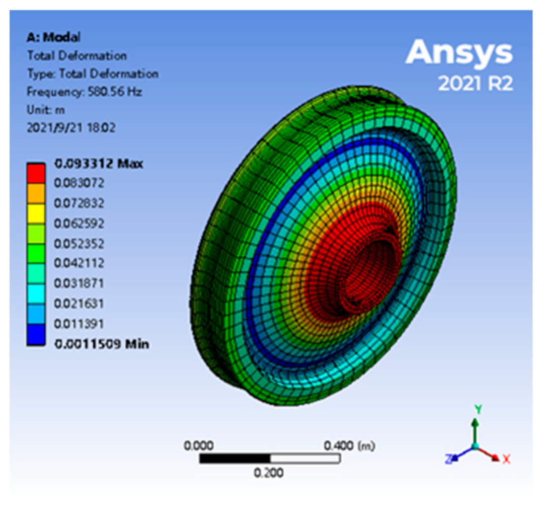
4.1. Wheel Modal Parameters

The CAD model of CRH₃ wheels was created and loaded into CAE tools for the first 16 modes’ analysis, the ninth of which is seen in Figure 3. The mode of this order can be observed to be wheel umbrella deformation, and the lateral deformation of the wheel hub is visible, which adds significantly to the lateral vibration. As a result of substituting the natural frequency (580.56 Hz) and modal mass (383 kg) of the mode of this order into Equation (20), the modal stiffness is 5.07 × 10⁹ N/m.

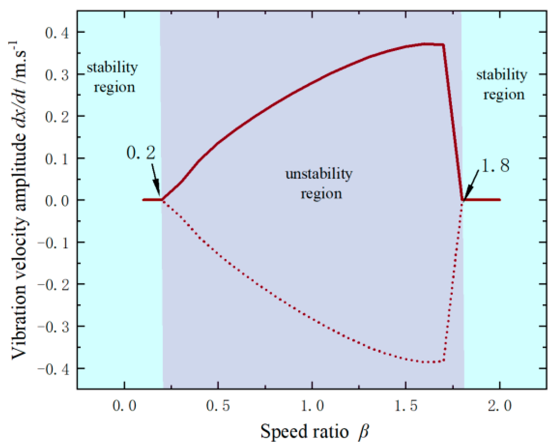
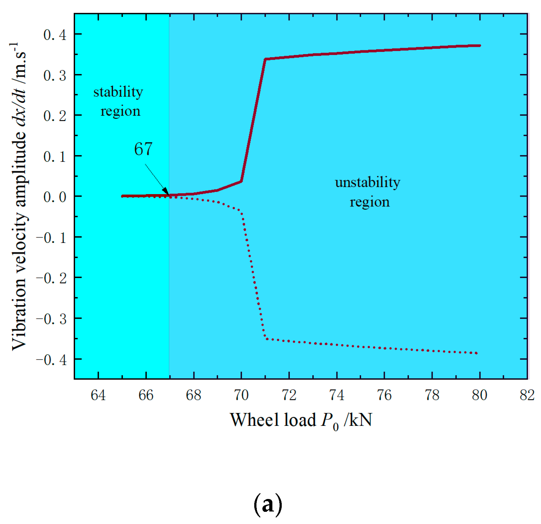
4.2. System Bifurcation Point Is Determined

Draw crucial curves for the speed ratio β, damping ratio ξ, and wheel load P₀, as indicated in Figure 4. The parameter domain is divided into three sections by the critical border of parameters β and P: the area of β < β₁ and β > β₂ is stable, while the region of β₁ < β < β₂ is unstable. The instability zone grows as P₀ increases.

The alterations in the ξ–β critical curve are comparable to those in the P₀–β critical curve. The instability zone shrinks fast as ξ increases. The vibration equation is solved and the impact of each parameter is explored to validate this result and determine the changing characteristics at the critical point.

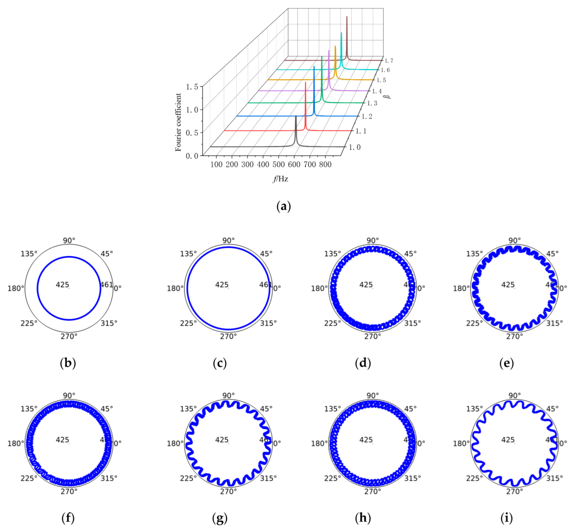
4.3. Influence of Parameters on Self-Excited Vibration Characteristics

4.3.1. Speed

Taking the speed ratio β = 0.1~2.0 to investigate the vibration characteristics at various rotating speeds, the bifurcation diagram in Figure 5 shows that, when the speed is low, the wheel cannot create self-excited vibration. When β = 0.2, the stable equilibrium point loses stability, and Hopf bifurcation leads to periodic oscillation, i.e., the wheel generates self-excited vibration. The system becomes stable again at β = 1.8 and is increased further.

The time domain diagrams and phase diagrams at different speeds in Figure 6 show that, when the speed is low (V = 36 km/h), the time domain diagrams increasingly converge. The stable focus in the phase diagram is the equilibrium point, and the wheel cannot create self-excited vibration. The time domain figure displays the constant amplitude and the phase diagram illustrates the elliptic limit cycle when V = 180 km/h. The system loses stability when the stable equilibrium point becomes unstable, and the wheel creates self-excited vibration. When the speed is increased further, to V = 324 km/h, supercritical Hopf bifurcation returns to the system. The time domain diagram progressively converges, the limit cycle disappears in the phase diagram, and the equilibrium point reverts to being the stable point. The system is generally stable, and the wheel cannot produce self-excited vibration.

As a result, while the vehicle is traveling at speeds ranging from 36 to 324 km/h, the wheel can create self-excited vibration, implying that polygonal wear may occur.

4.3.2. Wheel Load

The vibration characteristics of a wheel load at P₀ = 65~80 kN were investigated using β = 1.6. The bifurcation diagram in Figure 7 demonstrates this. With the increase in wheel load, the stable equilibrium point loses stability when P₀ = 67 kN, and Hopf bifurcation leads to periodic oscillation, that is, the wheel generates self-excited vibration.

When P₀ < 67 kN, the time domain graph progressively converges, the phase diagram’s equilibrium point is the stable focus, and the wheel cannot generate self-excited vibration. As the speed increases, the time domain graphic displays the constant amplitude waveform and the phase diagram reveals the elliptic limit cycle in P₀ > 67 kN. The system loses stability when the stable equilibrium point becomes the unstable focus, and the wheel creates self-excited vibration.

4.3.3. Wheel Rail Vertical Dynamic Force

Using a speed ratio β = 1.6 and a wheel load P₀ = 80 kN, the vibration characteristics are investigated using dynamic load coefficients k_d = 0.0025, 0.025, and 0.25, as well as frequency ratios n_d = 1 and 3.

The spectrum of the system with the amplitude and frequency of the wheel load dynamic load shown in Figure 8a,b shows that the wheel dynamic load excites the same frequency response. The amplitude of the wheel dynamic load influences the low-frequency response amplitude, and the frequency of the wheel dynamic load influences the low-frequency response frequency. Both have no effect on the size of higher-order frequency, implying that the vertical force of the wheel rail has no effect on the magnitude of fixed frequency. According to Figure 8c, the polygonal wear consists of a low order (3rd) with the same frequency as the wheel rail vertical force and a high order (20th) with the fixed frequency.

4.3.4. Damping Ratio

Taking speed ratio β = 1.6 and a wheel load of P₀ = 80 kN, the vibration characteristics are investigated for damping ratios ξ = 0~0.15.

The bifurcation diagram of the system changing with the damping ratio shown in Figure 9 shows that, when the damping ratio is small, the wheels generate self-excited vibration; when the damping ratio is increased to 0.09, subcritical Hopf bifurcation occurs, the equilibrium point becomes the stable focus, and the wheel does not generate self-excited vibration.

5. Evolution Verification of Wheel Polygonal Wear

5.1. Numerical Simulation Verification

The lateral creep force spectrum within the speed range of the self-excited vibration is drawn to verify the theoretical analysis conclusion that the wheel polygonal wear will evolve when the wheel rotational frequency is divided into the wheel lateral vibration frequency after the self-excited vibration of the wheel is generated, as shown in Figure 10a. The vibration frequency of the lateral creep force with periodic oscillation generated by Hopf bifurcation is independent of vehicle speed, and it is fixed around 588.47 Hz at various vehicle speeds. This finding is congruent with the conclusion in [20] that polygonal wheel wear is “frequency fixed”. Given the wheel mass and lateral stiffness, the lateral vibration frequency is $f_1=\frac{1}{2\pi }\sqrt{\frac{k_s}{m}}=580.4$ Hz. It is clear that the frequency corresponds to the natural frequency of wheel lateral vibration.

Furthermore, within the speed range that creates self-excited vibration, the lateral creep force is substituted into the wheel circumferential wear formula, and the polygon wear characteristics of the wheel are shown. The wear characteristics in Figure 10b–i show that, when the vehicle speed is 36 or 324 km/h, that is, when the wheel does not have lateral self-excited vibration, the circumferential wear is uniform. The wheel wear will finally be uniform after long-term operation when the vehicle speed is 198, 234, and 270 km/h; however, there are evenly distributed wear peaks in the wheel circumferential direction only when the vehicle speed is 252, 288, and 308 km/h. After a long period of operation, obvious regular 24th, 21st, and 20th order polygons will be formed, and the product of wheel rotational frequency and wear order is approximately equal to 588 Hz, indicating that the wheel polygonal wear exhibits the “divisible” feature.

To summarize, when the wheel has polygon wear, it exhibits “self-excitation—constant speed—fixed frequency—divisible” properties. That is, the incidence and evolution of wheel polygonal wear must fulfill the criteria that, while the wheel is moving at a constant speed, it creates self-excited periodic vibration with a constant frequency, and the frequency of the self-excited vibration is divided by the wheel rotational frequency. The findings of the simulation validate the theoretical analysis.

5.2. Actual Vehicle Tracking Verification

The CRH₃ EMU has a top speed of 300 km/h. According to field measurements, the wheel diameter life cycle has three stages of high-speed growth of polygonal wheel wear. The wheel diameters are 830, 875, and 915mm, respectively, corresponding to polygon wear of 18th, 19th, and 20th orders [2]. The rotational frequency f₂ and lateral vibration frequency f₁ of the matching wheelset may be estimated using the present vehicle recorded data, as given in

Table 1. Analysis of wheel polygonal wear parameters.

D/mm	ω/(rad·s−1)	f2/Hz	N	f1/Hz
915	182.1	29.0	20	580.1
875	190.5	30.3	19	576.3
830	200.8	32.0	18	575.6

.

Table 1 shows that polygonal wear occurs when the train is traveling at 300 km/h and the wheel diameters are 830, 875, and 915 mm, respectively. There is a constant frequency of 580 Hz in all three circumstances. The “fixed frequency” is equal to the multiple of the corresponding wheel rotational frequency, and the integral multiple causes 18th, 19th, and 20th order wheel polygon wear. It is clear from the measured data of current automobiles that the polygonal wear of wheels exhibits apparent “fixed frequency” features. This is consistent with the study result.

6. Conclusions

The properties of lateral self-excited vibration and polygonal wear of wheels are explored using the LuGre friction model and self-excited vibration theory, and the conditions for the generation and evolution of polygonal wear are disclosed. The following findings are reached after verifying the measured data of current vehicles:

• The dynamic model of the wheel lateral self-excited vibration is constructed, and the lateral self-excited vibration stability of the system is investigated. The Hopf bifurcation points are found for vehicle speed, dampening, and wheel load.
• It is discovered that the polygonal wear of the wheel exhibits “constant speed–self excitation–fixed frequency–divide” features. The existing vehicle tracking data had been confirmed.
• The order of the wheel is the ratio of the wheel lateral self-excited vibration frequency to its rotational frequency.
• The wheel–rail vertical dynamic force excites the same frequency low-order wheel polygon, but has little impact on the high-order wheel polygon, and its effect on wheel polygonal wear requires additional investigation.

References

1. Barke, D.W.; Chiu, W.K. A review of the effects of out-of-round wheels on track and vehicle components. Proc. Inst. Mech. Eng. Part F Rail. Rapid. Transit 2005, 219, 151–175. [Google Scholar] [CrossRef]
2. Jin, X.S.; Wu, Y.; Liang, S.L.; Wen, Z.F. Mechanisms and countermeasures of out-of-roundness wear on railway vehicle Wheels. J. Southwest Jiaotong Univ. 2018, 53, 1–14. (In Chinese) [Google Scholar]
3. Wang, P.; Tao, G.Q.; Yang, X.X.; Wen, Z.F. Analysis of Polygonal Wear Characteristics of Chinese High-Speed Train Wheels. J. Southwest Jiaotong Univ. 2021, 1–9. Available online: http://kns.cnki.net/kcms/detail/51.1277.U.20211124.1532.002.html (accessed on 21 July 2022). (In Chinese).
4. Tao, G.Q.; Wang, L.F.; Wen, Z.F.; Guan, Q.H.; Jin, X.S. Measurement and assessment of out-of-round electric locomotive wheels. Proc. Inst. Mech. Eng. Part F Rail. Rapid. Transit 2018, 232, 275–287. [Google Scholar] [CrossRef]
5. Wu, Y.; Du, X.; Zhang, H.J.; Wen, Z.F.; Jin, X.S. Experimental analysis of the mechanism of high-order polygonal wear of wheels of a high-speed train. J. Zhejiang Univ. Sci. A Appl. Phys. Eng. 2017, 18, 579–592. [Google Scholar] [CrossRef]
6. Nielsen, J.C.O.; Johansson, A. Out-of-round railway wheels—A literature survey. Proc. Inst. Mech. Eng. Part F Rail. Rapid. Transit 2000, 214, 79–91. [Google Scholar] [CrossRef]
7. Johansson, A.; Andersson, C. Out-of-round railway wheels—A study of wheel polygonalization through simulation of three-dimensional wheel-rail interaction and wear. Veh. Syst. Dyn. 2005, 43, 539–559. [Google Scholar] [CrossRef]
8. MORYS. Enlargement of out-of-round wheel profiles on high speed trains. J. Sound Vib. 1999, 227, 65–978. [Google Scholar]
9. Chen, G.X.; Jin, X.S.; Wu, P.B.; Dai, H.Y.; Zhou, Z.R. Finite element study on the generation mechanism of polygonal wear of railway wheels. J. China Railw. Soc. 2011, 33, 14–18. (In Chinese) [Google Scholar]
10. Zhao, X.N.; Chen, G.X.; Lv, J.Z.; Zhang, S.; Wu, B.W.; Zhu, Q. Studyon the mechanism for the wheel polygonal wear of high-speed trains in terms of the frictional self-excited vibration theory. Wear 2019, 426–427, 1820–1827. [Google Scholar] [CrossRef]
11. Cui, X.L.; Li, T.; Bao, P.; Wen, X.; Yang, Z. Research on the Dynamic Cause of Rail Corrugation in the Braking Section of High-Speed Railways Under Multiple Vibration Inducements. J. Vib. Eng Technol. 2022. [Google Scholar] [CrossRef]
12. Wu, B.W.; Qiao, Q.F.; Chen, G.X.; Lv, J.Z.; Zhu, Q.; Zhao, X.N.; Ouyang, H. Effect of the unstable vibration of the disc brake system of high-speed trains on wheel polygonalization. Proc. Inst. Mech. Eng. Part F Rail. Rapid. Transit 2020, 234, 80–95. [Google Scholar] [CrossRef]
13. Peng, B.; Iwnicki, S.; Shackleton, P.; Crosbee, D. Comparison of wear models for simulation of railway wheel polygonization. Wear 2019, 436–437, 203010. [Google Scholar] [CrossRef]
14. Fu, B.; Bruni, S.; Luo, S.H. Study on wheel polygonization of a metro vehicle based on polygonal wear simulation. Wear 2019, 438–439, 203071. [Google Scholar] [CrossRef] [Green Version]
15. Pombo, J.; Ambrósio, J.; Pereira, M.; Lewis, R.; Dwyer-Joyce, R.; Ariaudo, C.; Kuka, N. Development of a wear prediction tool for steel railway wheels using three alternative wear functions. Wear 2011, 271, 238–245. [Google Scholar] [CrossRef]
16. Dong, Y.H.; Cao, S.Q. Generation and evolution conditions of polygonal wear of high-speed wheel. Shock. Vib. 2021, 2021, 1–10. [Google Scholar] [CrossRef]
17. Ishikawa, Y.; Kawamura, A. Maximum Adhesive Force Control in Super High-Speed Train. In Proceedings of the Power Conversion Conference, Nagaoka, Japan, 6 August 1997; pp. 951–954. [Google Scholar]
18. Ye, Y.G.; Zhu, B.; Huang, P.; Peng, B. OORNet: A deep learning model for on-board condition monitoring and fault diagnosis of out-of-round wheels of high-speed trains. Measurement 2022, 199, 111268. [Google Scholar] [CrossRef]
19. De Wit, C.C.; Olsson, H.; Astrom, K.-J.; Lischinsky, P. A new model for control of systems with friction. IEEE Trans. Autom. Control. 1995, 40, 419–425. [Google Scholar] [CrossRef] [Green Version]
20. Wu, Y.; Jin, X.S.; Cai, W.B.; Han, J.; Xiao, X.B. Key Factors of the Initiation and Development of Polygonal Wear in the Wheels of a High-Speed Train. Appl. Sci. 2020, 10, 5880. [Google Scholar] [CrossRef]
Figure 1. Model of lateral self-excited friction vibration of wheel: (a) wheel–rail lateral self-excited vibration model; (b) wheel–rail friction self-excited vibration model.
Machines 10 00608 g001
Figure 2. Relationship curve between creep speed and creep coefficient of wheel-rail contact.
Machines 10 00608 g002
Figure 3. The ninth mode of the wheel mode.
Machines 10 00608 g003
Figure 4. Critical curve between parameters β and P0, ξ: (a) P0–β critical curve; (b) ξ–β critical curve.
Machines 10 00608 g004
Figure 5. Bifurcation diagram of the system with the variation in β.
Machines 10 00608 g005
Figure 6. Time domain diagram and phase diagram of wheel vibration at different speeds: (a) V = 36 km/h; (b) V = 180 km/h; and (c) V = 324 km/h.
Machines 10 00608 g006aMachines 10 00608 g006b
Figure 7. Influence of system with wheel load: (a) bifurcation diagram of the system; (b) time domain diagram and phase diagram at P0 = 67 kN; (c) time domain diagram and phase diagram at P0 = 80 kN.
Machines 10 00608 g007aMachines 10 00608 g007b
Figure 8. Effect of wheel rail vertical dynamic force: spectrum diagram under (a) nd = 3 and (b) kd = 0.25; wear characteristic under (c) nd = 3 and kd = 0.25.
Machines 10 00608 g008
Figure 9. Bifurcation diagram of the system with the damping ratio.
Machines 10 00608 g009
Figure 10. Frequency spectrum and circumferential wear shape under difference speed: (a) frequency spectrum; circumferential wear shape at (b) β = 0.2 (V = 36 km/h); (c) β = 1.8 (V = 324 km/h); (d) β = 1.1 (V = 198 km/h); (e) β = 1.2 (V = 216 km/h); (f) β = 1.3 (V = 234 km/h); (g) β = 1.4 (V = 252 km/h); (h) β = 1.5 (V = 270 km/h); (i) β = 1.6 (V = 288 km/h).
Machines 10 00608 g010