Article

Risk Assessment Model-Guided Configuration Optimization for Free-Floating Space Robot Performing Contact Task

Key Laboratory of Space Utilization, Technology and Engineering Center for Space Utilization, Chinese Academy of Sciences, Beijing 100094, China
*
Author to whom correspondence should be addressed.
Machines 2022, 10(9), 720; https://doi.org/10.3390/machines10090720
Submission received: 30 June 2022 / Revised: 19 August 2022 / Accepted: 19 August 2022 / Published: 23 August 2022
(This article belongs to the Topic Recent Advances in Robotics and Networks)

Abstract

:
The use of free-floating space robots for contact tasks is very promising in space exploration. However, severe damage or obvious disturbance may occur if inappropriate operation is implemented. In this paper, a novel risk assessment method is first proposed to give a clear description of the risk state before contact happens and provide guidance for configuration optimization to reduce risk on contact tasks. Firstly, the dynamics model of a free-floating space robot is given. On this basis, two important risk assessment indicators, the maximum contact force and the base attitude disturbance caused by contact, are derived. By integrating the risk assessment indicators, a novel risk assessment model is proposed for a free-floating space robot performing a contact task. It is a multidimensional and extensible risk assessment space which could give a clear description of the risk state before contact happens. Thereafter, considering the results given by the risk assessment model, the configuration optimization for a free-floating space robot is implemented based on the design of optimization factor in null space. Finally, numerical simulation for a 7-degree-of-freedom free-floating space robot performing a contact task is carried out, and the simulation results verify the effectiveness of the proposed method.

1. Introduction

In the past decades, space robots have been playing an important role in space contact tasks, such as on-orbit construction and assembly, target capture and asteroid sampling [1,2,3]. During the contact process, there are two major problems, namely, the maximum contact force and the base attitude disturbance caused by contact, that need to be focused on. If the maximum contact force exceeds the limit that the space robot allows, the robot itself or the target may be damaged. When the inertia of the base is not large enough, the eccentric external force and torque will cause an obvious base attitude disturbance, which will affect the communication with the ground and power supply for the space robot, and compensating for the disturbance using the attitude control system will consume a large amount of fuel, which is limited in space. Therefore, the minimization of maximum contact force and the minimization of base attitude disturbance attract the attention of scholars.
On the basis of the assumption that the contact is an instantaneous phenomenon, and the contact effect can be regarded as a contact-–impact impulse applied on the end-effector, the contact model is then established by the theorem of impulse [4,5,6,7]. This method is called the discrete contact dynamics modeling method, which can realize the simple and efficient contact dynamics analysis of space robots. However, it can only obtain the final changes of the space robotic system caused by contact and cannot obtain the information during the entire contact process, including the maximum contact force. Thereafter, the null-space optimization methods for redundant space robots or the intelligent optimization methods are adopted to minimize the contact-impact impulse by adjusting capture configuration [8,9,10,11]. However, as the contact-impact impulse is the integration of the contact force over the entire contact period, the minimization of the contact-impact impulse is not equivalent to the minimization of the maximum contact force. In order to obtain the information during contact process, a continuous contact analysis method needs to be introduced. A general and comprehensive analysis on continuous contact force models based on Hertz’s law combined with the hysteresis damping factor is present in [12,13,14], and these models can be directly applied to the space robotic system by measuring the relative indentation on the contact point [15,16,17]. This method requires all the motion equations of robotic system integrated over the entire period of contact, and thus it can provide accurate results but may not be very efficient. With the assumption that the duration of contact period is small enough that the configuration and the direction of contact remain the same during the contact period, an effective mass concept is proposed to analyze the contact process of the space robot performing the contact task [18,19]. This method can improve the computational efficiency, and give an analytic solution of the contact information, but there exist singularity problems for certain configurations, and for the space robot in free-floating mode, especially with the initial velocity of the base, there exists an obvious error of the contact information. In the follow-up research, Zhang solves the problems of singularity and obvious errors for certain cases by introducing the base attitude variable into the integrated effective mass and gives the analytical expression of the maximum contact force under non-central contact for the first time [20].
For the minimization of the base attitude disturbance, compensation mechanisms, such as base-mounted reaction wheel and balance arm, are proposed by some scholars [21,22,23]. However, there may be several drawbacks for these compensation mechanisms. Firstly, the overall mass of the space robotic system is increased. Secondly, their capacity to compensate for the base attitude disturbance is limited. Thirdly, the complexity of the space robotic system is increased, which is not preferred in the control scheme. Therefore, the methods by planning the robotic manipulator motion to minimize the base attitude disturbance are also proposed. Some scholars derived the motion coupling relationship between the free-floating base and robotic manipulator based on the conservation of momentum and angular momentum and used this coupling relationship to plan the motion of the robotic manipulator to reduce the base attitude disturbance [24,25,26,27]. However, the base attitude disturbance caused by contact is not considered in the coupling motion planning methods above. The contact dynamics analysis of a free-floating space robot subject to a force impulse at the end-effector is presented in [28], where the preferable directions of the contact force are defined as the directions that can minimize the impact moment transfer toward the base. Based on this idea, a “straight arm capture” concept is proposed in [29,30]. By configuration optimization, no base attitude disturbance exists when the direction of the contact force is along the line connecting the centroid of the robotic manipulator and the centroid of the base. The direct mapping relationship between the base attitude disturbance and the contact-impact impulse is established in [31], and the goal of reducing base attitude disturbance is achieved by designing the null-space configuration optimization factor.
The above optimization methods for reducing the maximum contact force and the base attitude disturbance are beneficial for the free-floating space robot performing contact tasks. However, existing research is mainly aimed at optimizing a single objective of the two risk assessment indicators, and the optimization objective is described in a qualitative statement as “as small as possible”. Since the two risk assessment indicators are not consistent or even opposite in some configurations, it cannot be ensured that by optimizing one indicator, the two indicators can meet the requirements at the same time. For example, when the space robot is fully stretched to contact the target, it conforms to the concept of straight-arm capture, which can make the base attitude undisturbed. However, this configuration will cause a significant increase in the maximum contact force. At the same time, the risk has rarely been assessed before performing the contact task, which is actually a necessary part. According to the risk assessment results, it can be judged whether the contact task needs to be optimized or whether the contact task can be successfully performed, even after optimization.
To the best of our knowledge, this is the first contact risk assessment method proposed for a free-floating space robot performing a contact task. The maximum contact force and the base attitude disturbance are considered simultaneously to form a multi-dimensional risk assessment space. It can objectively describe the risk level of the space robot performing contact tasks and provide guidance for the optimization of risk assessment indicators. The rest of this paper is organized as follows. The dynamics model of a free-floating space robot is given in Section 2. On this basis, two important risk assessment indicators, the maximum contact force and the base attitude disturbance caused by contact, are derived in Section 3. Section 4 provides a novel risk assessment method which could give a clear description of the risk state before contact happens and the corresponding operation suggestions. A configuration optimization method guided by the risk assessment model is proposed in Section 5. The effectiveness of the proposed method is verified by numerical simulations in Section 6. Finally, conclusions are drawn in Section 7.

2. Dynamics Model of Free-Floating Space Robot

A general model of free-floating space robot with n revolute joints is shown in Figure 1, where Σ I is the inertial frame, Σ B is the base frame, Σ E is the end-effector frame, Σ i is the ith joint frame with z axis representing the rotation direction (i = 1, 2, …, n), r 0 is the position vector of the origin of base frame, a i is the vector from the origin of joint frame i to the centroid of link i, b 0 is the vector from the origin of base frame to the origin of joint frame 1, and b i is the vector from the centroid of link i to joint frame i + 1. p i , p e are the position vectors of joint i and the end-effector, respectively.
The position vector of the centroid of link i is
r i = r 0 + k = 1 i a k + k = 0 i 1 b k
The angular velocity and the linear velocity of link i are
ω i = ω 0 + k = 1 i z k θ ˙ k
v i = v 0 + ω 0 × r i r 0 + k = 1 i z k × r i p k θ ˙ k
where ω 0 , v 0 are the angular velocity and the linear velocity of the base, z k is the unit vector of the kth joint rotation direction, and θ ˙ k is the kth joint angular velocity.
The kinetic energy of a free-floating space robot is expressed as
T = 1 2 i = 0 n ω i T I i ω i + m i v i T v i
where m 0 , I 0 are the mass and inertia matrix of the base, and m i , I i are the mass and inertia matrix of the ith link with i = 1 ~ n.
Substituting Equations (2) and (3) into Equation (4), it can be obtained that
T = 1 2 v 0 T , ω 0 T , θ ˙ T H v 0 ω 0 θ ˙
where θ ˙ = θ ˙ 1 , θ ˙ 2 , , θ ˙ n T and H is called the system inertial matrix with specific expression as follows.
H = [ M E M r 0 g × T i = 1 n m i J ν i M r 0 g × i = 0 n I i + m i r 0 i × T r 0 i × i = 1 n I i J ω i m i r 0 i × T J ν i i = 1 n m i J ν i T i = 1 n J ω i T I i m i J ν i T r 0 i × i = 1 n J ω i T I i J ω i + m i J ν i T J ν i ]
where M represents the total mass of the system, E is an identity matrix, r 0 g is the vector from the origin of the base frame to the mass centroid of the system, r 0 i is the vector from the origin of the base frame to the centroid of link i, and r × is the skew symmetric matrix of vector r . The linear velocity Jacobian matrix and angular velocity Jacobian matrix corresponding to the ith link centroid each has the following expression.
J ν i = z 1 × r i p 1 , z 2 × r i p 2 , , z i × r i p i , 0 , , 0 3 × n
J ω i = z 1 , , z i , 0 , , 0 3 × n
The potential energy is neglected, as the system is in a microgravity environment and the flexible characteristics of the joints and links are not considered. Substituting Equation (5) into the Lagrange equation, the dynamics model governing the motion of a free-floating space robot can be obtained [32,33].
H ϕ ¨ + C = F b _ m + J b _ m T F e
where ϕ ¨ = x ¨ b T , θ ¨ T T with x ¨ b = v ˙ 0 T , ω ˙ 0 T T and θ ¨ = θ ¨ 1 , θ ¨ 2 , , θ ¨ n T , and C = c b T , c m T T with c b , c m is the velocity-dependent nonlinear terms of the base and the manipulator. F b _ m = F b T , τ m T T with F b = f b T , τ b T T is the external force/torque applied on the base and τ m an n-dimensional vector of control torques applied at the joints. F e = f e T , τ e T T is the external force/torque applied on the end-effector, and J b _ m = J b , J m with J b , J m is the Jacobian matrices of the base and the manipulator, respectively.

3. Contact Risk Assessment Indicators

Recall the note that when a free-floating space robot performs a contact task, two main aspects need special attention, namely the maximum contact force and the base attitude disturbance caused by contact. In the following, the two key indicators will be obtained by specific theoretical derivation.

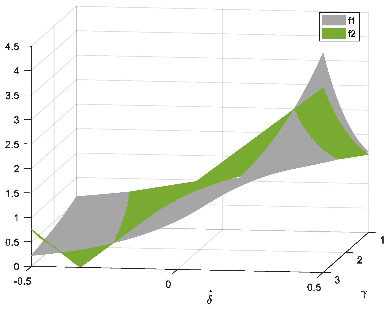
3.1. The Maximum Contact Force

Generally, the contact happens at the end-effector when performing tasks, and thus the study of effective mass perceived at the end-effector will be focused on. The linear and the angular velocity of the end-effector can be calculated by
ω e = ω 0 + k = 1 n z k θ ˙ k
v e = v 0 + ω 0 × p e r 0 + k = 1 n z k × p e p k θ ˙ k
Combing Equations (10) and (11), it can be obtained that
x ˙ e = J b x ˙ b + J m θ ˙ = J b _ m ϕ ˙
where x ˙ e = v e T , ω e T T , ϕ ˙ = x ˙ b T , θ ˙ T T with x ˙ b = v 0 T , ω 0 T T .
Considering the dynamics model of the free-floating space robot, as the inertial matrix H is invertible, multiply J b _ m H 1 on both sides of Equation (9) and combine Equation (12), the dynamics model with respect to the variables of the end-effector can be obtained.
H ^ x ¨ e + C ^ = F ^ b _ m + F e
where H ^ = J b _ m H 1 J b _ m T 1 , C ^ = J b _ m T C H ^ J ˙ b _ m ϕ ˙ , F ^ b _ m = J b _ m T F b _ m with J b _ m T is the generalized inverse of J b _ m T .
The analysis of the inertial properties perceived at the end-effector depends on the study of matrix H ^ [19,34]. The effective mass perceived at the end-effector can be expressed as
m e = 1 u T H ^ ν 1 u
where u is the unit direction vector of the applied force, H ^ ν = J b _ mv H 1 J b _ mv T 1 with J b _ mv representing the linear velocity Jacobian matrix.
On this basis, the free-floating space robot can be regarded as a single body from the perspective of the end-effector. When performing the contact task, the effective mass m e can be directly substituted into the contact model to obtain the information during contact process.
The classical model of the continuous contact force between two bodies is shown in Equation (15) which incorporates a spring and a damper in parallel connecting the contact point [13,35].
F = Κ δ α + λ δ α δ ˙
where δ is the relative indentation between contacting bodies and δ ˙ is the velocity of relative indentation, λ is the hysteresis damping factor, Κ and α are the contact stiffness parameter and the nonlinear power exponent determined from material and geometric properties of the local region of the contacting bodies. α is generally set to be 1.5 [36], and Κ becomes the function of curvature radius R 1 , R 2 at the contact point.
Κ = 4 3 π σ 1 + σ 2 R 1 R 2 R 1 + R 2
where σ i is the material parameter related to the Young’s modulus E i and Poisson’s ratio ς i ,
σ i = 1 ς i 2 π E i , i = 1 , 2
From Equation (15), the following mathematical representation of the dynamics system can be obtained.
M r δ ¨ + λ δ α δ ˙ + Κ δ α = 0
where δ ¨ is the acceleration of relative indentation, M r = m e m t / m e + m t with m e the effective mass perceived at the end-effector and m t the target mass.
Through some mathematical manipulation, the expression of relative indentation can be obtained.
δ α + 1 = M r α + 1 λ 2 λ δ ˙ δ ˙ ( ) + K ln λ δ ˙ + K λ δ ˙ ( ) + K
where δ ˙ ( ) is the initial relative contact velocity.
Substituting δ ˙ = 0 into Equation (19), the maximum deformation can be expressed as
δ max = M r α + 1 λ 2 λ δ ˙ ( ) + K ln K λ δ ˙ ( ) + K 1 α + 1
And the analytical expression of the maximum contact force can be approximately expressed as [20]
F max = Κ M r α + 1 λ 2 λ δ ˙ ( ) + K ln K λ δ ˙ ( ) + K α α + 1 .
In order to obtain the information of the entire contact process, Equation (19) needs to be solved. Substituting δ = 0 into Equation (19), the following transcendental equation can be obtained:
e γ δ ˙ = γ δ ˙ + 1 γ δ ˙ ( ) + 1 e γ δ ˙ ( )
where γ = λ / K .
The two functions f 1 δ ˙ , γ = e γ δ ˙ and f 2 δ ˙ , γ = γ δ ˙ + 1 / γ δ ˙ ( ) + 1 e γ δ ˙ ( ) are shown in Figure 2 with δ ˙ 0.5 , 0.5 m/s, γ 1 , 3 and δ ˙ ( ) = 0.4 m/s. The intersection points of the two functions are the solution of Equation (22). When δ = 0 , there should be two values of δ ˙ , namely δ ˙ ( ) and δ ˙ ( + ) which means the instantaneous velocity when the contacting bodies depart. However, it can be seen that the number of solutions is also related to γ , e.g., there are three solutions when γ = 3 . Therefore, necessary constraints must be added to Equation (22).
In fact, the value of γ is not selected randomly, and it depends on K and λ as the definition. The calculation of K is discussed above. The energy loss during the contact process can be quantified by calculating the changes of the system energy by the concept of restitution coefficient c r or the work of the damping force, and based on this theory, there are several expressions of the hysteresis damping factor λ , which are named after the proposers as shown in Table 1 [12,13,14].
It can be seen that the models of the hysteresis damping factor have the following expression form.
λ = f c r K δ ˙ ( )
Thus,
γ = λ K = f c r δ ˙ ( )
The value of γ depends on restitution coefficient c r and initial relative contact velocity δ ˙ ( ) . Based on this, two constraints are added to Equation (22): Constraint 1. The value of γ should be obtained by Equation (24); Constraint 2. The absolute value of any solution should be less than δ ˙ ( ) based on the fact that there exists energy loss during contact process.
However, which model is the perfect one to be employed should be analyzed. A model selection method is proposed in the following. It is known that restitution coefficient c r is used to describe the velocity relationship before and after contact. δ ˙ t ( + ) = c r δ ˙ ( ) is used to calculate the ideal post-contact velocity, and based on Equation (22), a model-based post-contact velocity defined by δ ˙ m ( + ) can also be obtained. Therefore, the model error can be evaluated by comparing the deviation of the post-contact velocities as follows.
ξ = δ ˙ m ( + ) δ ˙ t ( + ) δ ˙ t ( + ) × 100 % = c r _ m c r c r × 100 %
where c r _ m = δ ˙ m ( + ) / δ ˙ ( ) .
When δ ˙ = δ ˙ m ( + ) , the following equation can be obtained from Equation (22).
e λ K δ ˙ m ( + ) δ ˙ ( ) = λ δ ˙ m ( + ) + K λ δ ˙ ( ) + K
Combining Equations (22) and (24)–(26), it can be obtained that
e f c r 1 + ξ c r 1 = f c r 1 + ξ c r + 1 f c r + 1 , c r _ m c r e f c r 1 ξ c r 1 = f c r 1 ξ c r + 1 f c r + 1 , c r _ m < c r
Although it is very hard to show an intuitive relationship between c r and ξ , it can be concluded that ξ is only dependent on c r . Based on the analysis, c r and ξ are respectively used as the input and the output to draw Figure 3.
From Figure 3, it can be seen that the Hunt-Crossley, Herbert-McWhannell, Lee- Wang, and Lankarain-Nikravesh models are more suitable for the case with high input restitution coefficient, and conversely, the Gharib-–Hurmuzlu model is suitable for the case with low input restitution coefficient. The Gonthier et al. model, Flore et al. model, Hu-–Guo model and Zhang et al. model have better performance over the entire range. Generally, the restitution coefficient can be known in advance based on the contact environment, and in order to obtain more accurate information during the contact period, a suitable model with the smallest model error should be selected according to the input restitution coefficient.
Further, from Equation (19), the contact time can also be obtained.
t = λ 2 M r α + 1 2 α α + 1 δ ˙ ( ) δ ˙ d δ ˙ λ δ ˙ + K M r λ δ ˙ δ ˙ ( ) + K ln λ δ ˙ + K λ δ ˙ ( ) + K α α + 1
Equation (28) describes the contact duration time. When δ ˙ = 0 , t means the duration time during the compression phase, and when δ ˙ = δ ˙ + , t means the duration time during the entire contact process.
So far, the contact time, the relative indentation and the velocity of relative indentation can all be obtained, and through the contact force model Equation (15), the continuous contact force during the entire contact period can be obtained.

3.2. The Base Attitude Disturbance Caused by Contact

Rewrite the dynamics model as [31]
M E M r 0 g × T H b m ν M r 0 g × H ω H b m ω H b m ν T H b m ω T H m v ˙ 0 ω ˙ 0 θ ¨ + c b ν c b ω c m = f b τ b τ m + J b ν T J b ω T J m T F e
where H b m ν = i = 1 n m i J ν i , H b m ω = i = 1 n I i J ω i m i r 0 i × T J ν i , H ω = i = 0 n I i + m i r 0 i × T r 0 i × , H m = k = 1 n J ω k T I k J ω k + m k J ν k T J ν k , H m = k = 1 n J ω k T I k J ω k + m k J ν k T J ν k , c b ν , c b ω are the linear and angular velocity-dependent nonlinear terms of the base, J b ν , J b ω are the linear and angular Jacobian matrices of the base.
Equation (29) is reformulated with respect to the base attitude and the joint angles by eliminating the base linear velocity acceleration term v ˙ 0 .
H ˜ ω H ˜ b m ω H ˜ b m ω T H ˜ m ω ˙ 0 θ ¨ + c ˜ b ω c ˜ m = τ ˜ b τ ˜ m + J ˜ b ω T J ˜ m T F e
where H ˜ ω = H ω + M r 0 g × r 0 g × , H ˜ b m ω = H b m ω r 0 g × H b m ν , H ˜ m = H m H b m ν T H b m ν / M , c ˜ b ω = c b ω r 0 g × c b ν , c ˜ m = c m H b m ν T c b ν / M , τ ˜ b = τ b r 0 g × f b , τ ˜ m = τ m H b m ν T f b / M , J ˜ b ω T = J b ω T r 0 g × J b ν T , J ˜ m T = J m T H b m ν T J b ν T / M .
Eliminate θ ¨ in Equation (30), and it can be obtained that
H ^ ω ω ˙ 0 + c ^ b ω = τ ^ b + J ^ b ω T F e
where H ^ ω = H ˜ ω H ˜ b m ω H ˜ m 1 H ˜ b m ω T , c ^ b ω = c ˜ b ω H ˜ b m ω H ˜ m 1 c ˜ m , τ ^ b = τ ˜ b H ˜ b m ω H ˜ m 1 τ ˜ m , J ^ b ω T = J ˜ b ω T H ˜ b m ω H ˜ m 1 J ˜ m T .
For the free-floating space robot, no external force/torque is applied on the base and thus f b = 0 , 0 , 0 T , τ b = 0 , 0 , 0 T . Integrate Equation (31) over an infinitesimally small time period Δ t from an arbitrary time t 0 and cancel the velocity-dependent terms and internal forces and replace all accelerations with the respective finite changes of velocity which will be denoted as δ . The following equation can be obtained.
δ ω 0 = H ^ ω 1 J ^ b ω T t 0 t 0 + Δ t F e d t
where Δ t means the duration time during the entire contact period and F e means the contact force, which can be both obtained from the continuous contact model derived in Section 3.1.

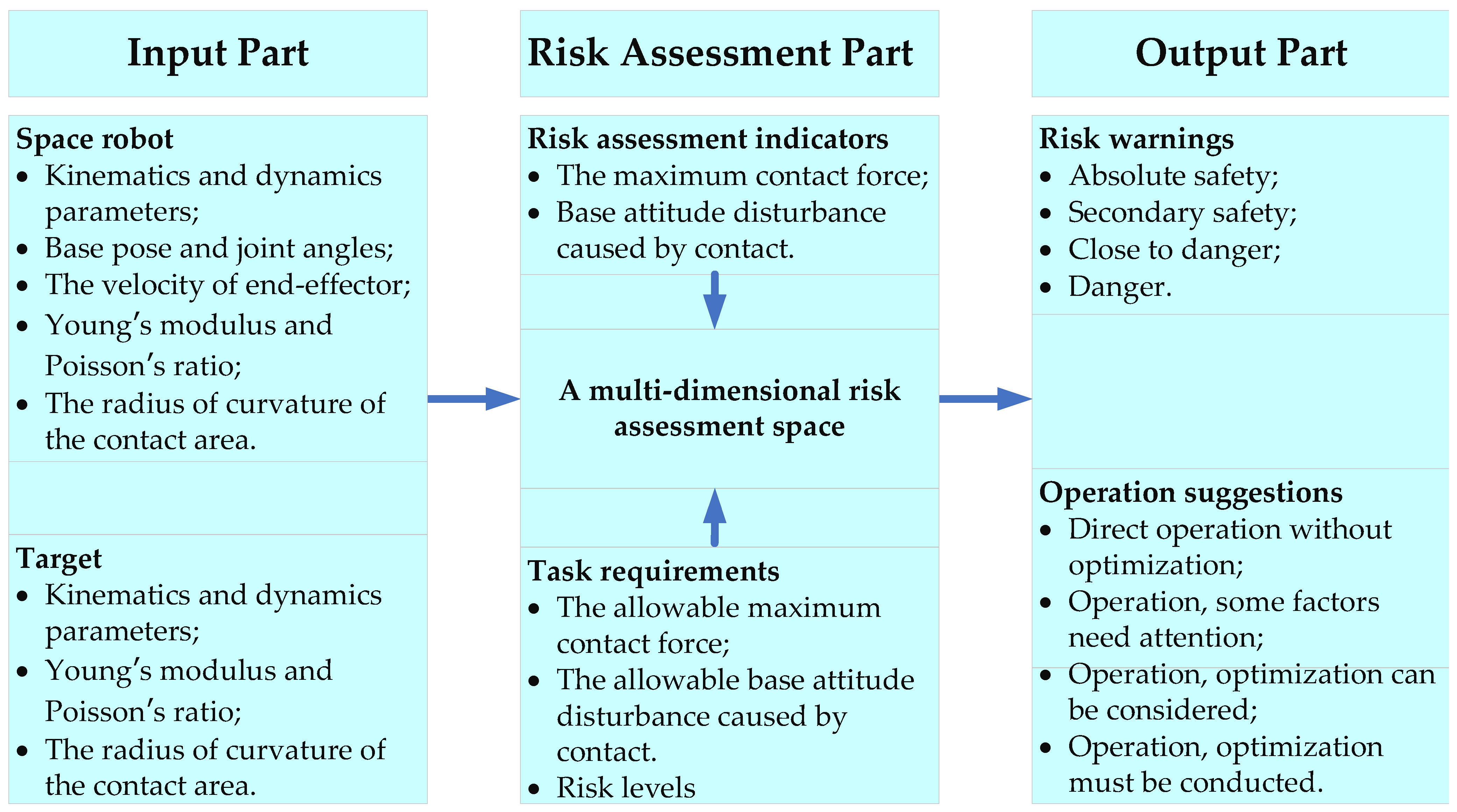
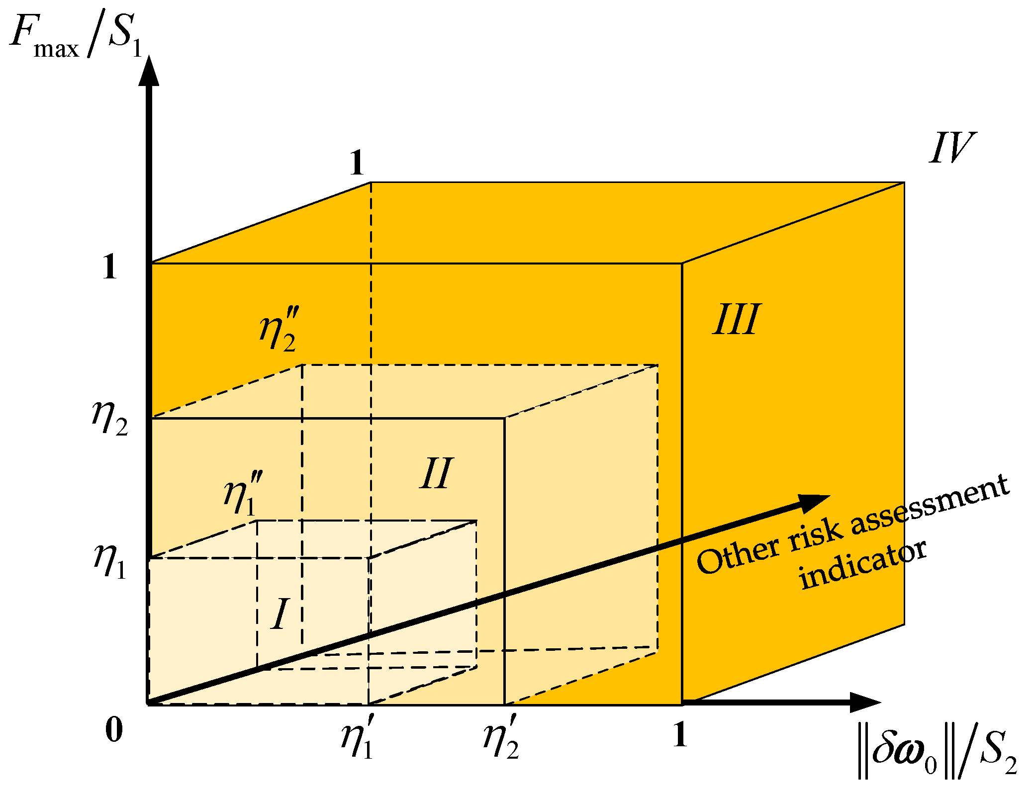
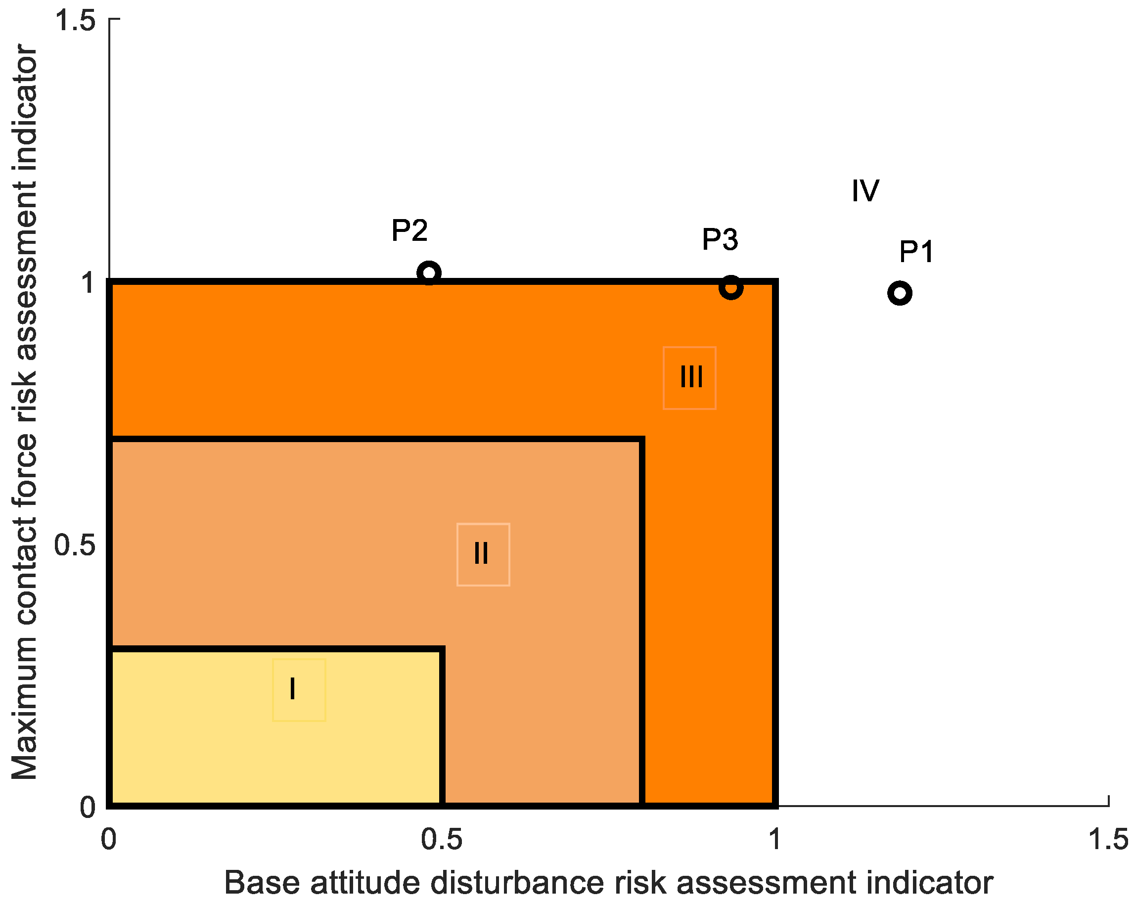
4. Contact Risk Assessment Model

As shown in Figure 4, the risk assessment method proposed in this paper mainly consists of three parts: the input part, the risk assessment part and the output part. Pre-contact information of the space robot and the target is needed in the input part. It includes the kinematics and dynamics parameters of the space robot, the base pose and the joint angles, the velocity of the end-effector, and the mass and velocity of the target. The above input information can be used to calculate the value of the effective mass perceived at the end-effector of the space robot. The Young’s modulus, Poisson’s ratio and the radius of curvature of the contact area are needed to obtain the hysteresis damping factor and the contact stiffness parameter. The risk assessment indicators which are developed in Section 3.1 and Section 3.2 are both included in the risk assessment part. By combining the mechanical design standard or the task requirements, the risk warnings and the corresponding operation suggestions are given in the output part.
It is assumed that four risk levels and two risk indicators are considered in the risk assessment part, and the corresponding two-dimensional risk assessment space is shown in Figure 5 with its x-axis representing the base attitude disturbance indicator and y-axis representing the maximum contact force indicator. S 1 is the allowable maximum contact force on the end-effector and S 2 is the 2-norm of the allowable maximum base attitude disturbance. Therefore, F max / S 1 0 , 1 and δ ω 0 / S 2 0 , 1 are the necessary conditions to ensure the safety of the contact tasks. η 1 , η 2 and η 1 , η 2 are the threshold values which need to be pre-determined for each indicator based on the mechanical design standard or the task requirements. Four risk levels are explained as follows.
Risk I. F max / S 1 0 , η 1 and δ ω 0 / S 2 0 , η 1 .
For most contact tasks performed by a space robot, F max / S 1 and δ ω 0 / S 2 are expected to be as small as possible. Therefore, Risk I actually means absolute safety, and the operation suggestion is direct operation without further optimization.
Risk II. F max / S 1 η 1 , η 2 and δ ω 0 / S 2 0 , η 2 ; F max / S 1 0 , η 2 and δ ω 0 / S 2 η 1 , η 2 .
Risk II means secondary safety, and the operation suggestion is operation with the attention on the indicators, which exceeds the absolute safety zone.
Risk III. F max / S 1 η 2 , 1 and δ ω 0 / S 2 0 , 1 ; F max / S 1 0 , 1 and δ ω 0 / S 2 η 2 , 1 .
When F max / S 1 1 or δ ω 0 / S 2 1 , it means that F max or δ ω 0 is close to its limit. Therefore, Risk III means close to danger, and the operation suggestion is operation and that some optimization strategies can be considered.
Risk IV. F max / S 1 1 , + ; δ ω 0 / S 2 1 , + .
In this condition, F max or δ ω 0 exceeds its limit, which will lead to the failure of the contact task. Therefore, Risk IV means danger, and the operation suggestion is stop and that optimization strategies must be conducted until the risk assessment result is satisfying.
If there are three risk assessments indicators, the three-dimensional risk assessment space is shown in Figure 6. The points in different cubes represent different risk levels. If there are more than three risk assessments indicators, a multi-dimensional risk assessment space is shown in Figure 7 with five risk assessment indicators in total and two kinds of risk levels. There are four risk levels for risk assessment indicators 1–4, and three risk levels for risk assessment indicator 5. The steps to make a multi-dimensional risk assessment space are as follows:
Step 1: Draw coordinate axes according to the number of risk assessment indicators, and each coordinate axis represents a risk assessment indicator.
Step 2: Normalize each risk assessment indicator and mark them on the coordinate axis according to the risk levels (the yellow circle in Figure 7).
Step 3: Correspondingly connect the risk level points of each risk assessment indicator from the highest risk level to the lowest risk level. If the risk levels of each risk assessment indicators are inconsistent, the insufficient risk level points are replaced by the lowest risk level point.
Step 4: According to the parameters in the input part and the calculation method in the risk assessment part of the risk assessment model, the values of each risk assessment indicator are marked on the corresponding axis as the red marker ‘*’ in Figure 7.
Step 5: If all risk assessment indicators fall within Risk I, it means absolute safety. If the risk assessment indicators are in different risk levels, the highest risk level shall prevail.
Step 6: If the value of all risk assessment indicators does not exceed 1, then the contact task can be performed, and it is better to properly optimize for the close-to-danger indicators. If at least one risk assessment indicator is in risk level IV, then the task must be stopped until the optimization results meet the requirements.

5. Contact Risk Assessment Model-Guided Configuration Optimization

Figure 8 shows the flow chart of the risk assessment model-guided configuration optimization. Firstly, a multi-dimensional risk assessment space is established according to the risk assessment indicators and task requirements. Secondly, according to the pre-contact parameters of the free-floating space robot, the risk level of the contact task is judged to determine whether it needs to be optimized. Thirdly, if the task is judged as not to be optimized by the risk assessment model, then it is operated directly. If the task is judged to need optimization, the risk assessment model-guided optimization method is used to optimize the contact configuration of the free-floating space robot. Finally, re-judge whether the optimized contact configuration meets the risk level. If the task requirements are still not satisfied, the task cannot be performed. The null-space optimization method with self-regulation weights is derived in detail as follows.
According to Equation (12), the non-minimum-norm solutions based on the Jacobian pseudoinverse can be written in the following form:
ϕ ˙ = J b _ m x ˙ e + k E J b _ m J b _ m ε
where, J b _ m is the pseudoinverse of J b _ m , E J b _ m J b _ m is the null space of J b _ m , k is the gain coefficient and ε is the optimization factor in null space. The velocities in null space produce a change in the configuration of space robot without affecting its velocity at the end-effector. To ensure that the capture pose of the end-effector is not affected by the configuration optimization, set x ˙ e = 0 , 0 , 0 , 0 , 0 , 0 T in Equation (33).
ϕ ˙ = k E J b _ m J b _ m ε
For reducing the base attitude disturbance caused by contact, the following optimization function is defined according to Equation (32).
f 1 = δ ω 0
For reducing the maximum contact force, its optimization function is
f 2 = F max = Κ M r α + 1 λ 2 λ δ ˙ ( ) + K ln K λ δ ˙ ( ) + K α α + 1
Combining Equations (35) and (36), the optimization factor is designed as
ε = k 1 ε 1 + k 2 ε 2
where ε 1 = f 1 x b , f 1 y b , f 1 z b , f 1 α , f 1 β , f 1 γ , f 1 θ 1 , , f 1 θ n T , ε 2 = f 2 x b , f 2 y b , f 2 z b , f 2 α , f 2 β , f 2 γ , f 2 θ 1 , , f 2 θ n T , x b , y b , z b , α , β , γ represents the pose of the base, k 1 and k 2 are the weights which are designed as follows.
k 1 = 0 1 δ ω 0 S 2 Δ 2 1 F max S 1 Δ 1 + δ ω 0 S 2 Δ 2 2 δ ω 0 S 2 Δ 2 1 δ ω 0 S 2 Δ 2 > 1 , F max S 1 Δ 1 1 δ ω 0 S 2 Δ 2 > 1 , F max S 1 Δ 1 > 1 , k 2 = 0 1 F max S 1 Δ 1 1 F max S 1 Δ 1 + δ ω 0 S 2 Δ 2 2 F max S 1 Δ 1 1 F max S 1 Δ 1 > 1 , δ ω 0 S 2 Δ 2 1 F max S 1 Δ 1 > 1 , δ ω 0 S 2 Δ 2 > 1
where Δ 1 , Δ 2 are the safety thresholds.
Equation (38) means that when the risk assessment indicator is in Risks I–III, the contact task can be directly performed without optimization. When the risk assessment indicator is in Risk IV, the optimization for the indicator must be conducted. If more than one risk assessment indicator needs to be optimized, the weights are set according to the proportion exceeding the risk value, which can realize self-regulation.

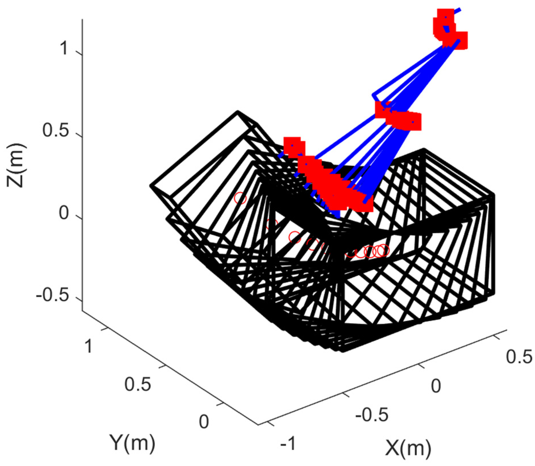
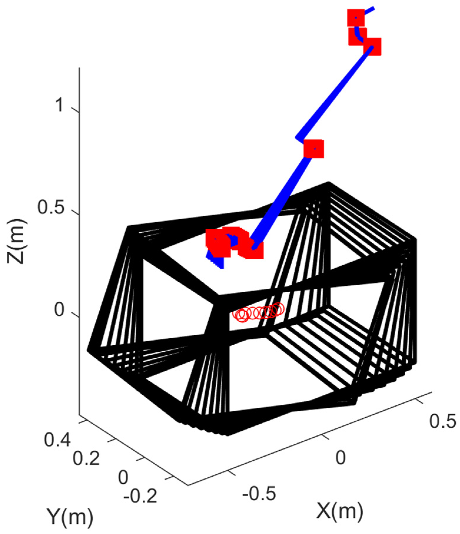
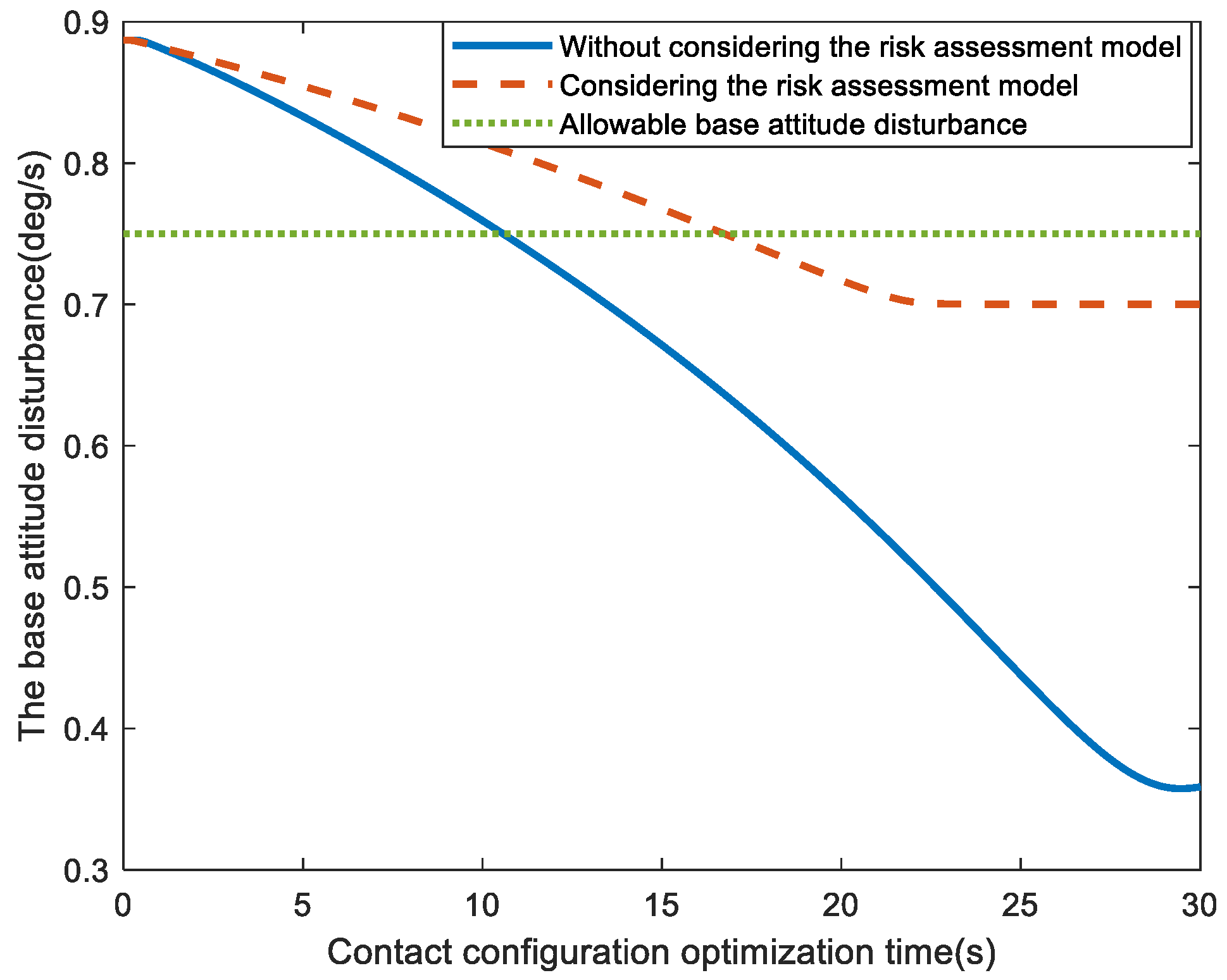
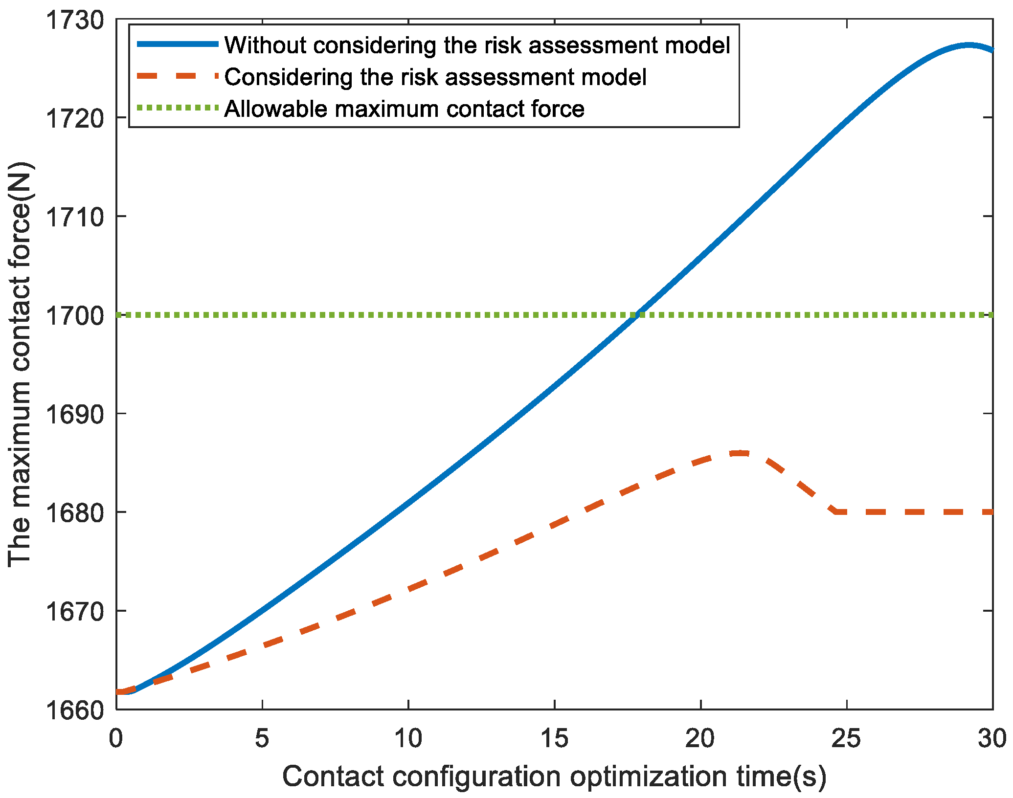
6. Numerical Simulations

The robot with a 7-DOF humanoid arm structure is one of the most representative space robots. It has redundant characteristics relative to the task space, can flexibly complete various tasks and has a wide range of application prospects. The famous space robot Canadarm2 has the same structure [37]. At the same time, the optimization method proposed in this paper also requires the space robot to have redundant characteristics. Therefore, a 7-DOF free-floating space robot as shown in Figure 9 is studied, where a = 0.4 m, b = 0.3 m, c = 0.1 m, d = 0.1 m, e = 0.5 m, f = 0.1 m, g = 0.5 m, h = 0.1 m, k = 0.1 m, and l = 0.1 m. Its dynamics parameters are listed in Table 2.
The initial contact configuration is [0,90,50,–10,58,90,0]deg, and the position and Euler angle of the base are [0,0,0]m and [0,0,0]deg, respectively, as shown in Figure 10. The other parameters related to the continuous contact model are set as u = 0.99 , 0 , 0.14 T , c r = 0.8 , K = 10 9   N / m 1.5 , δ ( ) = 0.1   m / s , m t = 60   kg , and the Zhang et al. model in Table 1 is selected as the hysteresis damping factor. The entire contact process can be calculated by the derivation in Section 3, which can help to obtain the maximum contact force of 1661.78 N and the base attitude disturbance of 0.89 deg/s. Assume that the allowable maximum contact force is 1700 N and the allowable base attitude disturbance is 0.75 deg/s, then set Δ 1 = 20 N and Δ 2 = 0.05 deg/s for safety. The risk assessment space with η 1 = 0.3 , η 2 = 0.7 , η 1 = 0.5 ,   η 2 = 0.8 is shown in Figure 11. Point p 1 represents the risk location corresponding to the above condition. It belongs to Risk IV, which means dangerous, and the risk assessment indicator of base attitude disturbance must be optimized.
In the first case, the optimization does not consider the risk assessment model, and only optimizes the base attitude disturbance. The optimization process is shown in Figure 12. The contact configuration is optimized without affecting the end-effector pose. In the second case, the risk assessment model-guided optimization method with self-regulation weights proposed in the paper is adopted, considering both the base-attitude-disturbance indicator and the maximum-contact-force indicator. The optimization process is shown in Figure 13. The contact configuration is optimized without affecting the end-effector pose.
Figure 14 and Figure 15 show the comparison of the optimization with and without considering the risk assessment model. For the optimization case without considering the risk assessment model, the base attitude disturbance is reduced from 0.89 deg/s to 0.36 deg/s, which meets the requirement of being below 0.75 deg/s as shown in Figure 14. However, the two risk assessment indicators are not consistent, because the optimization of the base-attitude-disturbance indicator causes the maximum-contact-force indicator to become worse. It can be seen from Figure 15 that the corresponding maximum contact force during the base attitude disturbance optimization increases from 1661.78 N to 1726.92 N, which does not meet the requirement of being below 1700 N. Point p 2 in Figure 11 represents this risk location. For the optimization case, considering the risk assessment model, the base attitude disturbance is reduced from 0.89 deg/s to 0.70 deg/s, and the maximum contact force increases from 1661.78 N to 1685.98 N and then decreases to 1680.00 N under the effect of weight self-regulation. Point p 3 in Figure 11 represents this risk location; both the risk assessment indicators meet the requirements, and the contact task can be performed by the free-floating space robot. Therefore, it is necessary to consider the risk assessment model in the optimization process. When setting the optimization parameters, the maximum allowable value of the risk assessment indicators can be set to other risk level thresholds according to the task requirements.

7. Conclusions

In order to improve the risk cognition and self-optimizing ability of a free-floating space robot when performing contact tasks, a novel risk assessment method is first proposed in this paper. It is a muti-dimensional and extensible risk assessment space which can give a clear description of the risk status before contact happens and provide guidance for configuration optimization to reduce risk on contact tasks. In this paper, two major risk assessment indicators, namely the maximum contact force and the base attitude disturbance, are integrated into the risk assessment model to form a two-dimensional risk assessment space. In order to make both risk assessment indicators meet the task requirements, a risk assessment model-guided configuration optimization method with self-regulation weights is proposed. The numerical simulation results verify the effectiveness of the proposed method.
The risk assessment model and the risk assessment model-guided configuration optimization method with self-regulation weights are the main contributions of the paper. The risk assessment model is common to both redundant and non-redundant space robots. It is extensible and can be integrated into more risk indicators to form a multi-dimensional risk assessment space. At present, the paper only considers the two risk indicators of the base attitude disturbance and the maximum contact force. In the future, more risk assessment factors, such as the joint torque and manipulability, will be considered. For the risk assessment model-guided configuration optimization method, it is only applicable to redundant space robots due to the use of null-space optimization algorithm. If there is a need to carry out the risk assessment model-guided configuration optimization for a non-redundant space robot, the task constraints can be reduced to form available null space.

Author Contributions

Conceptualization, L.Z. and S.W.; funding acquisition, L.Z.; methodology, L.Z.; writing—original draft, L.Z.; writing—review and editing, S.W. All authors have read and agreed to the published version of the manuscript.

Funding

This research was funded by National Natural Science Foundation of China, grant number 61903354.

Institutional Review Board Statement

Not applicable.

Informed Consent Statement

Not applicable.

Data Availability Statement

The data used to support the findings of this study are included within the paper.

Acknowledgments

Thanks to the reviewers who provided insight and expertise that greatly assisted in revising the manuscript.

Conflicts of Interest

The authors declare no conflict of interest.

References

  1. Xue, Z.H.; Liu, J.G.; Wu, C.C.; Tong, Y.C. Review of In-Space Assembly Technologies. Chin. J. Aeronaut. 2021, 24, 21–47. [Google Scholar]
  2. Zhu, A.; Ai, H.; Chen, L. A Fuzzy Logic Reinforcement Learning Control with Spring-Damper Device for Space Robot Capturing Satellite. Appl. Sci. 2022, 12, 2662. [Google Scholar] [CrossRef]
  3. Flores-Abad, A.; Ou, M.; Pham, K.; Ulrich, S. A Review of Space Robotics Technologies for On-Orbit Servicing. Prog. Aerosp. Sci. 2014, 68, 1–26. [Google Scholar]
  4. Yoshida, K.; Dragomir, N. Space Robot Impact Analysis and Satellite-Base Impulse Minimization Using Reaction Null-Space. In Proceedings of the IEEE International Conference on Robotics and Automation, Nagoya, Japan, 21–27 May 1995; pp. 1271–1277. [Google Scholar]
  5. Chen, G.; Jia, Q.X.; Sun, H.X.; Hong, L. Analysis on Impact Motion of Space Robot in the Object Capturing Process. Jiqiren 2010, 32, 432–438. [Google Scholar] [CrossRef]
  6. Raina, D.; Gora, S.; Maheshwari, D.; Shah, S.V. Impact Modeling and Reactionless Control for Post-Capturing and Manoeuvring of Orbiting Objects Using a Multi-Arm Space Robot. Acta. Astronaut. 2021, 182, 21–36. [Google Scholar] [CrossRef]
  7. Fan, M.; Tang, L. Impact Analysis and Trajectory Planning Stabilization Control for Space Robot after Capturing Target. Yuhang Xuebao 2021, 42, 1305–1316. [Google Scholar]
  8. Wee, L.B.; Walker, M.W. On the Dynamics of Contact Between Space Robots and Configuration Control for Impact Minimization. IEEE Trans. Rob. Autom. 1993, 9, 581–591. [Google Scholar]
  9. Jia, Q.X.; Zhang, L.; Chen, G.; Sun, H.X. Pre-Impact Trajectory Optimization of Redundant Space Manipulator with Multi-Target Fusion. Yuhang Xuebao 2014, 35, 639–647. [Google Scholar]
  10. Hu, J.C.; Wang, T.S. Pre-Impact Configuration Designing of a Robot Manipulator for Impact Minimization. J. Mech. Robot. 2017, 9, 031010. [Google Scholar] [CrossRef]
  11. Zhang, L.; Jia, Q.X.; Chen, G.; Sun, H.X. The Precollision Trajectory Planning of Redundant Space Manipulator for Capture Task. Adv. Mech. Eng. 2014, 6, 371673. [Google Scholar] [CrossRef]
  12. Machado, M.; Moreira, P.; Flores, P.; Lankarani, H.M. Compliant Contact Force Models in Multibody Dynamics: Evolution of the Hertz Contact Theory. Mech. Mach. Theory. 2012, 53, 99–121. [Google Scholar]
  13. Flores, P.; Machado, M.; Miguel, T.S.; Martins, J.M. On the Continuous Contact Force Models for Soft Materials in Multibody Dynamics. Multibody. Syst. Dyn. 2011, 25, 357–375. [Google Scholar] [CrossRef]
  14. Zhang, J.; Li, W.H.; Zhao, L.; He, G.P. A Continuous Contact Force Model for Impact Analysis in Multibody Dynamics. Mech. Mach. Theory 2020, 153, 103946. [Google Scholar] [CrossRef]
  15. Fang, Q.; Cui, M.M. Space Robot Capture Collision Force Control Method Based on Explicit Force Control. Chin. Space Sci. Technol. 2019, 39, 1–10. [Google Scholar]
  16. Ji, H.W.; Li, M.; Wang, X.C.; Li, Y.; Dou, L.H. Contact-Impact Dynamics Simulation for Space Manipulator Using Equivalent Spring-Damping Model. In Proceedings of the World Congress on Intelligent Control and Automation, Shenyang, China, 29 June–4 July 2014; pp. 3186–3191. [Google Scholar]
  17. Wu, S.; Mou, F.L.; Liu, Q.; Cheng, J. Contact Dynamics and Control of a Space Robot Capturing a Tumbling Object. Acta Astronaut. 2018, 151, 532–542. [Google Scholar] [CrossRef]
  18. Zhang, L.; Jia, Q.X.; Chen, G.; Sun, H.X.; Cao, L.F. Impact Analysis of Space Manipulator Collision with Soft Environment. In Proceedings of the 9th IEEE Conference on Industrial Electronics and Applications, Hangzhou, China, 9–11 June 2014; pp. 1965–1970. [Google Scholar]
  19. Jia, Q.X.; Zhang, L.; Chen, G.; Sun, H.X. Collision Analysis of Space Manipulator Multibody System Based on Equivalent Mass. Yuhang Xuebao 2015, 36, 1356–1362. [Google Scholar]
  20. Zhang, L. Configuration Optimization for Free-Floating Space Robot Capturing Tumbling Target. Aerospace 2022, 9, 69. [Google Scholar] [CrossRef]
  21. Shi, L.L.; Katupitiya, J.; Kinkaid, N. A Robust Attitude Controller for a Spacecraft Equipped with a Robotic Manipulator. In Proceedings of the American Control Conference, Boston, MA, USA, 6–8 July 2016; pp. 4966–4971. [Google Scholar]
  22. Dimitrov, D.N.; Yoshida, K. Utilization of the Bias Momentum Approach for Capturing a Tumbling Satellite. In Proceedings of the IEEE/RSJ International Conference on Intelligent Robots and Systems, Sendai, Japan, 28 September–2 October 2004; pp. 3333–3338. [Google Scholar]
  23. Han, D.; Huang, P.F.; Liu, X.Y.; Yang, Y. Combined Spacecraft Stabilization Control After Multiple Impacts During the Capture of a Tumbling Target by a Space Robot. Acta. Astronaut. 2020, 176, 24–32. [Google Scholar] [CrossRef]
  24. Xie, Y.R.; Wu, X.D.; Inamori, T.; Shi, Z.; Sun, X.Z.; Cui, H.T. Compensation of Base Disturbance Using Optimal Trajectory Planning of Dual-Manipulators in a Space Robot. Adv. Space Res. 2019, 63, 1147–1160. [Google Scholar] [CrossRef]
  25. Yan, L.; Xu, W.F.; Hu, Z.H.; Liang, B. Multi-Objective Configuration Optimization for Coordinated Capture of Dual-Arm Space Robot. Acta Astronaut. 2020, 167, 189–200. [Google Scholar]
  26. Zhang, Q.; Wang, L.; Zhou, D.S. Trajectory Planning of 7-DOF Space Manipulator for Minimizing Base Disturbance. Int. J. Adv. Rob. Syst. 2016, 13, 44. [Google Scholar] [CrossRef]
  27. James, F.; Shah, S.V.; Singh, A.K.; Madhava, K.K.; Misra, A.K. Reactionless Maneuvering of a Space Robot in Precapture Phase. J. Guid. Control. Dyn. 2016, 39, 2417–2423. [Google Scholar] [CrossRef]
  28. Nenchev, D.N.; Yoshida, K. Impact Analysis and Post-Impact Motion Control Issues of a Free-Floating Space Robot Subject to a Force Impulse. IEEE Trans. Rob. Autom. 1999, 15, 548–557. [Google Scholar] [CrossRef]
  29. Cong, P.C.; Sun, Z.W. Pre-Impact Configuration Planning for Capture Object of Space Manipulator. In Proceedings of the International Symposium on Systems and Control in Aerospace and Astronautics, Shenzhen, China, 10–12 December 2008; p. 4776179. [Google Scholar]
  30. Cong, P.C.; Zhang, X. Preimpact Configuration Analysis of a Dual-Arm Space Manipulator with a Prismatic Joint for Capturing an Object. Robotica 2013, 31, 853–860. [Google Scholar] [CrossRef]
  31. Zhang, L.; Jia, Q.X.; Chen, G.; Sun, H.X. Pre-impact Trajectory Planning for Minimizing Base Attitude Disturbance in Space Manipulator Systems for a Capture Task. Chin. J. Aeronaut. 2015, 28, 1199–1208. [Google Scholar] [CrossRef]
  32. Liang, B.; Xu, W.F. Space Robotics: Modelling, Planning and Control; Tsinghua University Press: Beijing, China, 2017; pp. 125–143. [Google Scholar]
  33. Xu, W.F.; Liang, B.; Li, C.; Liu, Y.; Xu, Y.S. Autonomous Target Capturing of Free-Floating Space Robot: Theory and Experiments. Robotica 2009, 27, 425–445. [Google Scholar] [CrossRef]
  34. Khatib, O. Inertial Properties in Robotic Manipulation. An Object-level Framework. Int. J. Rob. Res. 1995, 14, 19–36. [Google Scholar] [CrossRef]
  35. Hertz, H. Über Die Berührung Fester Elastischer Körper. J. Reine Angew. Math. 1881, 92, 156–171. [Google Scholar]
  36. Flores, P.; Ambrósio, J.; Claro, J.C.P.; Lankarani, H.M. Contact-Impact Force Models for Mechanical Systems. In Kinematics and Dynamics of Multibody Systems with Imperfect Joints: Models and Case Studies; Friedrich, P., Peter, W., Eds.; Springer: Berlin, Germany, 2008; Volume 34, pp. 47–56. [Google Scholar]
  37. Chen, G.; Zhang, L.; Jia, Q.X.; Sun, H.X. Singularity Analysis of Redundant Space Robot with the Structure of Canadarm2. Math. Probl. Eng. 2014, 2014, 735030. [Google Scholar] [CrossRef]
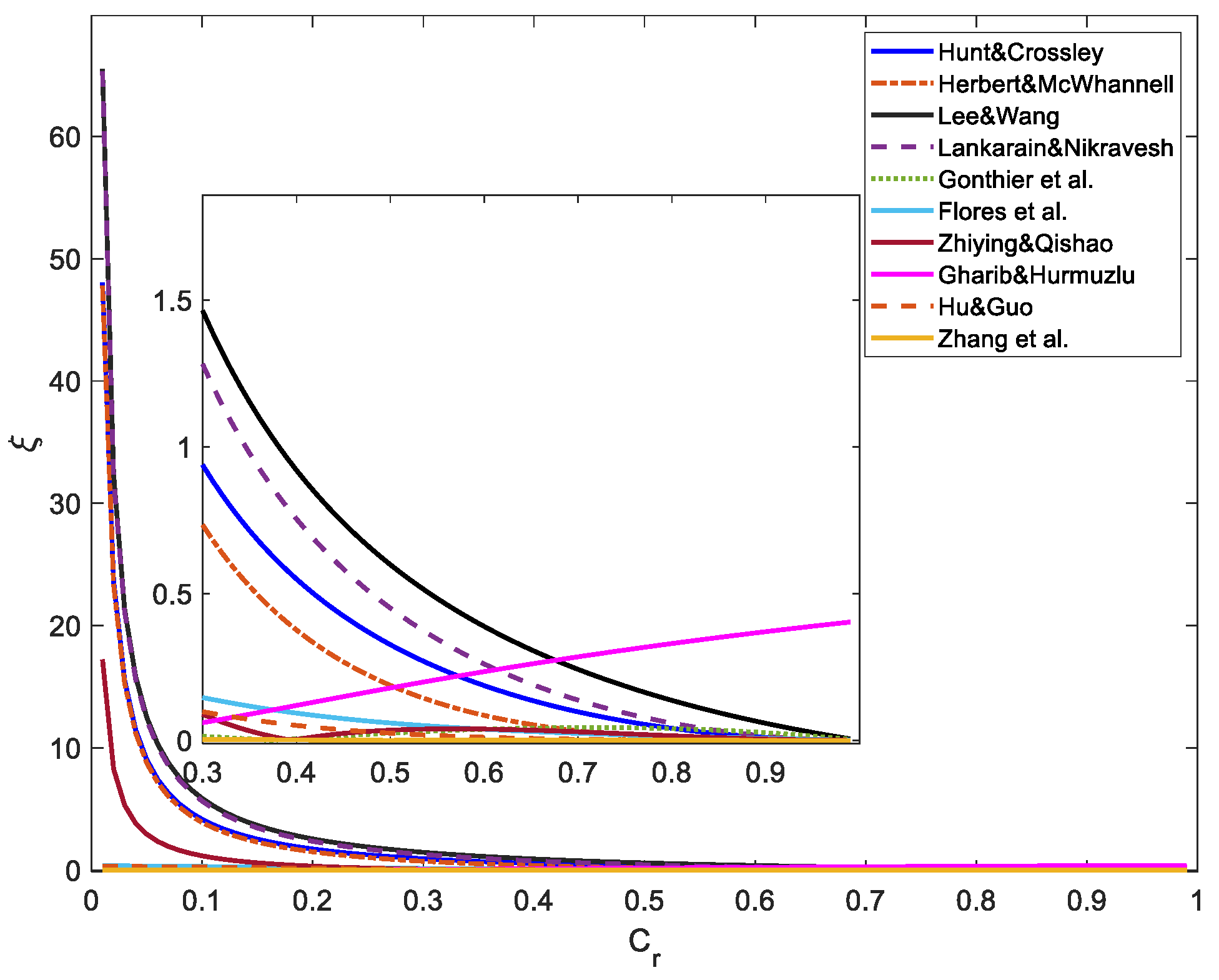
Figure 1. A general model of free-floating space robot.
Machines 10 00720 g001
Figure 2. The surfaces of f 1 and f 2 with respect to γ and δ ˙ .
Machines 10 00720 g002
Figure 3. The relationship between c r and ξ .
Machines 10 00720 g003
Figure 4. Three parts of proposed risk assessment method.
Machines 10 00720 g004
Figure 5. Two-dimensional risk assessment space.
Machines 10 00720 g005
Figure 6. Three-dimensional risk assessment space.
Machines 10 00720 g006
Figure 7. Multi-dimensional risk assessment space.
Machines 10 00720 g007
Figure 8. Flow chart of risk assessment model-guided configuration optimization method.
Machines 10 00720 g008
Figure 9. A 7-DOF free-floating space robot.
Machines 10 00720 g009
Figure 10. Initial contact configuration of free-floating space robot.
Machines 10 00720 g010
Figure 11. The risk assessment results of contact task.
Machines 10 00720 g011
Figure 12. The configuration optimization process without considering the risk assessment model.
Machines 10 00720 g012
Figure 13. The configuration optimization process considering the risk assessment model.
Machines 10 00720 g013
Figure 14. The optimization of the base attitude disturbance with and without considering the risk assessment model.
Machines 10 00720 g014
Figure 15. The change of the maximum contact force with and without considering the risk assessment model.
Machines 10 00720 g015
Table 1. Classical expressions of hysteresis damping factor.
ModelHysteresis Damping FactorModelHysteresis Damping Factor
Herbert–McWhannell λ = 6 1 c r 2 c r 1 2 + 3 K δ ˙ ( ) Hunt-Crossley λ = 3 1 c r 2 K δ ˙ ( )
Lankarain–Nikravesh λ = 3 1 c r 2 4 K δ ˙ ( ) Lee-Wang λ = 3 1 c r 4 K δ ˙ ( )
Flores et al. λ = 8 1 c r 5 c r K δ ˙ ( ) Gonthier et al. λ = 1 c r 2 c r K δ ˙ ( )
Zhiying–Qishao λ = 3 1 c r 2 e 2 1 c r 4 K δ ˙ ( ) Hu-Guo λ = 3 1 c r 2 c r K δ ˙ ( )
Zhang et al. λ = 3 1 c r 2 0.6181 e 3.52 c r + 0.899 e 0.09025 c r c r K δ ˙ ( ) Gharib–Hurmuzlu λ = 3 1 c r 2 c r K δ ˙ ( )
Table 2. Dynamics parameters.
PartMass (kg)Inertia Matrix (kg·m2)
Link 14diag ([0.50, 0.12, 0.50])
Link 24diag ([0.50, 0.12, 0.50])
Link 38diag ([0.46, 5.02, 5.02])
Link 48diag ([0.46, 5.02, 5.02])
Link 54diag ([0.50, 0.50, 0.12])
Link 64diag ([0.50, 0.50, 0.12])
Link 75diag ([0.50, 0.50, 0.12])
Base100diag ([50, 50, 50])
Publisher’s Note: MDPI stays neutral with regard to jurisdictional claims in published maps and institutional affiliations.

