Abstract
Rolling bearings are an important part of rotating machinery, and are of great significance for fault diagnosis and life monitoring of rolling bearings. Analyzing fault signals, extracting effective degradation information and establishing corresponding models are the premise of residual life prediction of rolling bearings. In this paper, first, the time-domain features were extracted to form the eigenvector of the vibration signal, and then the index representing the bearing degradation was found. It was found that the time-domain index could effectively describe the degradation information of the bearing, and the multi-dimensional time-domain characteristic information could effectively describe the attenuation trend of the vibration signal of the rolling bearing. On this basis, appropriate feature vectors were selected to describe the degradation characteristics of bearings. Aiming at the problems of large amounts of data, large amounts of information redundancy and unclear performance index of multi-dimensional feature vectors, the dimensionality of multi-dimensional feature vectors was reduced with principal component analysis, thus, simplifying the multi-dimensional feature vectors and reducing the information redundancy. Finally, in view of the support vector machine (SVM)’s needs to determine kernel function parameters and penalty factors, the squirrel optimization algorithm (SOA) was used to adaptively select parameters and establish the state-life evaluation model of rolling bearings. In addition, mean absolute error (MAE) and root mean squared error (RMSE) were used to comprehensively evaluate SOA. The results showed that the SOA reduced the errors by 5.1% and 13.6%, respectively, compared with a genetic algorithm (GA). Compared with particle swarm optimization (PSO), the error of SOA was reduced by 7.6% and 15.9%, respectively. It showed that SOA-SVM effectively improved the adaptability and regression performance of SVM, thus, significantly improving the prediction accuracy.
1. Introduction
The remaining useful life (RUL) estimation of rolling bearings is one of the key factors in condition-based maintenance, which began in the middle of the last century [1]. The acceleration sensor was used to obtain the acceleration signal of the bearing, and the working state of rolling bearings was determined by the peak change. In the past half-century, the theory of condition monitoring and life prediction of rolling bearings has been enriched, which provides a reliable basis for accurately predicting the RUL of rolling bearings.
The fatigue life of a rolling bearing refers to the working time or the total number of cycles of the bearing when the rolling element or any part from the inner and outer rings of the bearing falls off fatigue after the bearing is enabled. In order to obtain the characteristic points of the performance degradation of spatial rolling bearings and characterize the evolution trend of the life degradation of rolling bearings, it is impossible to rely on only a certain characteristic index, and a variety of characteristic indexes must be collected to comprehensively reflect their state [2]. At present, the main methods of rolling bearing life prediction are mechanical life prediction [3], probability and statistics life prediction [4] and new information technology life prediction [5].
Due to the difficulty of modeling, the traditional mechanical and probabilistic methods cannot be used in the actual equipment condition monitoring and life prediction. Therefore, intelligent condition monitoring has gradually become a hot topic in rolling bearing life prediction. Support vector machines (SVMs), neural networks, fuzzy calculations, genetic algorithms and so on have been widely used in the life prediction of rolling bearings. With the neural network algorithm, it is easy to fall into “over training” and “over learning”, which affects the generalization accuracy. Moreover, if the optimization parameters are selected incorrectly, the neural network will fall into a local minimum [6].
SVM was first proposed by Vapnik in 1995, which is a learning machine based on a VC dimension theory and a structural risk minimization principle [7]. It can effectively avoid the difficult problems of over-learning, under-learning, local minima and so on in neural network algorithms, and also has good generalization ability under the condition of small samples [8]. SVM plays an important role in pattern recognition, regression estimation and probability density function estimations. Sun et al. [9] used the SVM to predict bearing RUL and established a bearing life prediction model with high accuracy. Zhao et al. [10] used the least square support vector machine to predict the degradation performance of bearings. Chen et al. [11] successfully established the RUL model of space bearing by combining similarity theory with the SVM. Bao et al. [12] used the fuzzy support vector regression machine to predict the life degradation trend of slewing bearings, which can well predict the real-time life degradation trend.
Parameter optimization is the key factor for SVM classification performance. Some scholars have introduced the swarm intelligence algorithm to optimize the parameters of the SVM. Huang et al. [13] used the genetic algorithm (GA) to optimize SVM parameters, which effectively improved the classification performance of the SVM. However, due to the complex operations of the genetic algorithm, the optimization speed is slow. Feng et al. [14] proposed using particle swarm optimization (PSO) to optimize SVM parameters. Although the convergence speed was improved, it was easy to fall into local optimal solutions. Guermoui et al. [15] improved the artificial bee colony (ABC) algorithm to optimize the SVM, and achieved a more accurate performance. These intelligent algorithms have certain advantages in SVM parameter optimization, but at the same time, they have defects, such as slow optimization speed and can easily fall into local optimization.
In recent years, Xue et al. developed a novel swarm optimization approach, named sparrow search algorithm (SSA) [16]. SSA tested performance based on 19 benchmark functions. The results showed that the proposed SSA was superior to PSO, grey wolf optimizer (GWO) and gravitational search algorithm (GSA) in terms of accuracy, convergence speed, stability and robustness. However, when solving complex engineering optimization problems, the convergence speed of the algorithm decreases with the decrease in the search range in the later iterations. Moreover, with the decline of the sparrow population diversity, the population tends to be single. Then it can easily fall into local optimization, and jump repeatedly at the origin and the optimal position [17]. In addition, SSA has very good performance when solving the problem that the optimal solution is near the origin, which is far better than other algorithms. Nevertheless, SSA performs poorly when the optimal solution of the problem is far from the origin [18]. Since sparrow in SSA converges to the current optimal solution by jumping directly to the vicinity of the current optimal solution instead of moving to the optimal solution, this leads to SSA easily falling into the local optimal solution and its global search ability is weak [19].
Compared with precise algorithms, meta-heuristic algorithms rely less on mathematical modeling and derivation [20]. The RUL estimation of rolling bearings based on a meta-heuristic algorithm is a very rich field, and its application has been rapidly developed. Qiu et al. [21] proposed an ensemble RUL prediction model with GA, SVR, and WPHM, and the accuracy and effectiveness of the proposed method were validated by a bearing experiment. Souto et al. [22] compared two possible preprocessing techniques to improve the input quality of the PSO-SVM algorithm in the RUL prediction. Cheng et al. [23] developed a novel deep learning-based two-stage RUL prognostic approach by using fast search and find of density peaks clustering (FSFDPC) and a multi-dimensional deep neural network (MDDNN). Pan et al. [24] found a new method based on deep belief networks (DBNs) and improved the support vector data description (SVDD) in the rolling bearing performance degradation assessment, and introduced the SSA into the parameters optimization process of SVDD.
The squirrel optimization algorithm (SOA) [25] is also a simple and efficient new optimization algorithm, which has the characteristics of fast convergence and powerful optimizing ability. Unlike the SSA, the SOA gradually moves towards the optimal solution. As a new algorithm, it shows tremendous development potential. Jain et al. [25] proved that the performance of the SOA algorithm is better than some well-known meta-heuristic algorithms, such as GA and BA, by conducting optimization tests on 26 classical test functions and 7 CEC214 test set functions. Khare [26] used the method of experimental design to calibrate the parameters of the algorithm. On 240 randomly generated problems, the algorithm, including SOA was compared with five well-known meta-heuristic algorithms generated in recent years. Experiments showed that SOA had better robustness under the same accuracy, which indicated that the SOA algorithm may also have good effects on bearing life estimation. Sakthivel et al. [27] verified the practicability of the proposed algorithm on six different power test systems with different scales and complexity. Simulation results showed that the proposed SOA method was superior to other existing heuristic optimization techniques in terms of solution quality, robustness and computational efficiency. In the SOA algorithm, the seasonal change conditions were checked to prevent the algorithm from falling into local optimization. Basu [28] solved the complex economic dispatch problem of multi-regional cogeneration by the SOA. Through simulation experiments, it was verified that SOA had better performance than GWO, PSO, differential evolution (DE) and evolutionary programming (EP) algorithms.
In order to improve the accuracy of the bearing RUL prediction, this paper proposes to improve the SVM based on SOA. In the process of determining the relevant parameters of the model, the past algorithms were prone to falling into local optimization when optimizing the parameters. Therefore, in order to obtain the best bearing health index, determine the best model parameters and establish a high-precision and stable predictive performance model, the bearing degradation performance index model will be established based on the bearing performance index obtained from dimension reduction by principal component analysis (PCA). In addition, SOA, PSO and GA algorithms will be used to optimize SVM for bearing life prediction, and the prediction results of different models will be compared through the prediction evaluation index.
2. Feature Extraction and Pattern Recognition
2.1. Feature Extraction Based on Principal Component Feature Fusion
PCA is a common data analysis method that is used to reduce the dimensions of large datasets by reducing the number of indicators in the dataset and retaining most of the information on the indicators in the original dataset. PCA is applicable to dimensionality reduction technology on both labeled and unlabeled data [22]. This paper establishes the extraction method of feature information in the time-domain and frequency-domain, and then uses PCA to reduce the dimension of the feature vector set of bearing vibration signal extraction, which can effectively eliminate the redundancy in the original multi-dimensional feature information, and better characterize the rolling bearing fault information and life degradation trend.
As early as 1962, two American scholars first used the time-domain index to characterize the degradation characteristics. With the development of related theories, the application of time-domain characteristic parameters in engineering is increasing [29]. According to whether there are dimensions, time-domain signals can be divided into two categories: dimensional signals and dimensionless signals. Dimensional eigenvalues mainly include: maximum value, minimum value, peak value, mean value, variance, mean square value, root mean square, etc. The numerical value of the dimensional eigenvalue will change with the physical unit, which brings great difficulty to the operation. Therefore, dimensionless indexes are also used in signal analysis, such as peak index, pulse index, margin index, kurtosis index, waveform index and skewness. Set a signal{xn}(n = 1~N), where N is the number of sampling points, time domain signals used in this paper are shown in Table 1 and Table 2.

Table 1.
Calculation formula of dimensional indicators in time-domain signals.

Table 2.
Calculation formula of dimensionless indicators in time-domain signals.
This paper uses Cincinnati’s dataset [30] to verify the algorithm, and selects the sample data with a bearing speed of 2000 r/min and a sampling rate of 20 kHz. As is shown in Table 3, the data was collected 984 times, each time for 10 min, and the life cycle of the bearing was approximately 164 h.

Table 3.
The full-life cycle dataset.
Since the degradation characteristic information of rolling bearings is complex, with tendency and variability, if a single characteristic is selected as the attenuation index, the degradation information of bearings cannot be completely described. In order to obtain the characteristic points of the performance degradation of spatial rolling bearings and characterize the evolution trend of the life degradation of rolling bearings, some reliable time-domain characteristics were chosen in this paper: root mean square value, square root amplitude, absolute average value, variance, waveform index, skewness index, kurtosis index and so on.
The premise of using PCA is that there should be a strong linear correlation between the variables in the original data. If the linear correlations between the original variables are small and there is no simplified data structure for them, then PCA is virtually meaningless. Therefore, when applying PCA, we should first make a statistical test of its applicability. We set up a KMO (Kaiser-Meyer-Olkin-measure of sampling accuracy) test experiment. KMO is based on comparing the relative sizes of the simple correlation coefficients and the partial correlation coefficients between the original variables. When the square sum of partial correlation coefficients among all variables is far less than the square sum of simple correlation coefficients among all variables, the partial correlation coefficient between variables is very small, and the KMO value is close to 1. The variables are suitable for principal component analysis.
Kaiser gives the commonly used KMO measurement standard: a measurement of 0.9 or above indicates that it is very suitable; a measurement of 0.8 means suitable; a measurement of 0.7 means general; a measurement of 0.6 means not suitable; a measurement of 0.5 or less is extremely unsuitable. In our paper, the KMO of the selected multidimensional features is approximately 0.8 through the KMO test and experimental analysis, which is suitable for PCA analysis. In data dimension reduction processing in terms of time-domain features, the data features are very wide and highly correlated with each other. In the case of a large amount of data, it is easy to overfit the model. At this time, PCA analysis can be used to reduce the data dimension. The PCA method is used to fuse the time-domain feature indexes into the comprehensive feature indexes, and eliminate the insensitive redundant features hidden in the high-dimensional feature sets. In addition, we expect to obtain a one-dimensional curve describing the performance degradation of a rolling bearing, so that the index can better represent the operating state of the bearing and can be used as the evaluation index of bearing state change. This paper uses principal component analysis (PCA) to synthesize multiple characteristic indexes to reduce the dimension and form a principal component with more characteristics. The specific extraction process and algorithm design are as follows:
Step 1: Collect the full-cycle time-domain vibration signals, and convert the vibration signals into the index eigenvector group X.
Step 2: The eigenvector is normalized, and then transposed to obtain the standardized matrix N.
Step 3: The feature vector set is simplified by the PCA algorithm.
Step 4: According to the results of the PCA, the contribution rate, number and dimension of principal components are obtained.
Step 5: The full-cycle life decline index is analyzed based on the simplified eigenvector set.
In order to verify the prediction results, the sample points of the full-life cycle are divided into a test set and a training set 1:1, and the sample point interval becomes 20 min.
2.2. Pattern Recognition Based on SVM
In the field of pattern recognition, the accuracy of the SVM in speech recognition, face recognition, article classification and other fields has exceeded the traditional learning methods. SVM aims to find a balance between the complexity of the model and learning ability with limited sample information, so it has better generalization and adaptability in processing sample data [31].
The SVM is applied to the regression problem, which can retain all the main features [32]. Given the training data , a regression model will be achieved, with parameters w and b that make f(x) and y as close as possible [22]. The traditional regression model usually calculates the loss directly according to the difference between the model output f(x) and the actual output y. Only when f(x) and y are exactly the same, the loss is 0. Support vector regression (SVR) assumes that the absolute value of the difference between f(x) and y can be less than ϵ. Therefore, the SVR problem can be written as:
where, C is the penalty factor, is:
Introducing relaxation variables :
Then we can get:
Lagrange function is introduced to transform the optimization problem into a convex quadratic programming problem, and finally the dual form of the SVR is obtained:
where is a function, and α and are Lagrange operators:
The SVR solution is as follows:
where x is replaced by the kernel function ϕ (x), then the samples of the input space can be mapped to the high-dimensional feature space. The final model can be achieved:
If the kernel function K satisfies the Mercer condition,
Then only by introducing the kernel function to do an inner product operation in the original space, it is not necessary to calculate the specific form of nonlinear mapping Φ. Gaussian-radial basis function (RBF) is a commonly used kernel function:
2.3. Establish SOA-SVM Model
When using the kernel function, its parameters g and error penalty coefficient C have an important impact on the performance of the SVM. If not set properly, the model will overlearn. The SOA [25] uses the foraging strategy of flying squirrels as the principle to construct a mathematical model to find the best parameters. The principle is that there are n squirrels in the deciduous forest, and each squirrel stays on a tree. The fitness value of each squirrel’s location describes the level of food sources, namely, the best food source (pecan tree), normal food source (oak) and no food source (ordinary tree). Each squirrel looks for food alone and optimizes the use of food resources through dynamic foraging behavior. In the forest, there are only three types of trees, ordinary trees, oaks and pecans. The position of flying squirrels is represented by vectors in SOA and each vector has multiple dimensions. Therefore, flying squirrels can glide in one-dimensional, two-dimensional, three-dimensional or super-dimensional search spaces to change their own position.
The dimensionality reduction vector containing degradation features is divided into a training set and a test set according to parity 1:1. Then the SOA is used to automatically find out the optimal kernel function parameters and penalty factors, so as to establish an accurate prediction model and improve the adaptive ability of the SVM. Figure 1 is the flowchart of the SOA-SVM algorithm. The algorithm design steps are as follows:
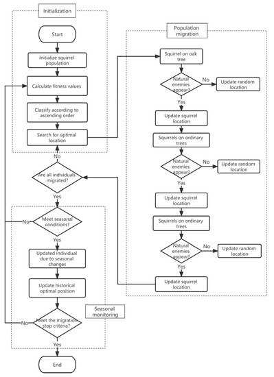
Figure 1.
The working process of the SOA-SVM algorithm.
Step 1: Define the input parameters, generate random positions in n squirrels, and evaluate the fitness value of each squirrel’s position. The positions of flying squirrels are arranged in ascending order by fitness.
Step 2: Define the population size, iteration times, sliding distance parameters and predator existence probability of the squirrel algorithm. Regression MSE is used as a fitness value and a fitness function. Determine the location of the hickory tree and the oak tree according to the MSE, that is, the location information of the global optimal solution and the local optimal solution.
Step 3: For squirrels still foraging in the forest, move closer to pecans and oaks, respectively. After updating the location information, calculate the seasonal monitoring value and compare it with the minimum seasonal constant. If the seasonal monitoring value is less than the minimum seasonal constant, the seasonal monitoring condition is true, and the squirrel that cannot search the forest can be relocated according to Levy’s flight.
Step 4: Repeat step 2 and step 3 until the iteration conditions are achieved or the maximum number of iterations is exceeded, and the optimization process is ended. Taking the squirrel position information on hickory trees as the global optimal solution, the adaptive SVM parameters C and g are obtained.
There are three main parameters in the SOA model: natural enemy occurrence probability, sliding scale factor and sliding constant. In this model, the squirrel’s sliding distance is in the range of 9–20 m. Too long a distance will cause great disturbance, which may lead to unsatisfactory performance of the algorithm. Therefore, dividing by a scale factor is helpful to realize the equilibrium state between global search and local optimization. Similar to the scale factor, the sliding constant achieves the balance between global search and local search, and the probability of natural enemies determines the moving strategy. Khare et al. [28] tested these three main parameters of the SOA algorithm by establishing comparative experiments. The algorithm had the best performance when the daily enemy occurrence probability was 0.15, the scale factor was 30, and the sliding constant was 1.5. In order to ensure the performance of the SOA, this paper adopted the same parameter settings for the SOA algorithm. In addition, the total number of individuals in the population was set to 20, the maximum number of iterations was set to 100, and the fitness function was set to MSE. Then, we performed a comparative experiment of PSO and GA, and set the experimental parameters. PSO was proposed by Kennedy and Eberhart in 1995. The idea of the algorithm is to search by particles, following the optimal particles in the solution space [33]. It is a classic case of using PSO to optimize SVM parameters. Yan Z et al. [34] improved and optimized the PSO algorithm to build a prediction model of the SVM in the bearing RUL prediction. In this experiment, there are three main parameters, two learning factors and inertia weight. Generally, the two learning factors are equal, and the range is between 0 and 4. The inertia weight of the other parameters affects the local search ability and the global search ability. When the inertia weight is small, it tends to exert the local search ability of PSO. When the inertia is large, the global search ability of the PSO algorithm will be emphasized. Generally, using 0.8 as the weight is a good choice, which can balance the local and global search [35]. Therefore, we set the parameter learning factor: the two learning factors are 2 and the weight is 0.8. We then chose the same fitness function, the population size was set to 20, and the iteration number was 100. Similarly, GA is a very classic heuristic intelligent algorithm. Due to its simplicity and rapidity, many scholars have applied it to the optimized SVM parameters [36]. In this comparative experiment, the main parameters of GA were as follows: the coding length was 20, the individual selection probability was 0.9, the same fitness function was selected, the population size was set to 20, and the iteration number was 100 [37].
In addition, in order to demonstrate the reliability of the heuristic algorithm experiment, the traditional grid search algorithm (GSA) was also used in the comparison test. The so-called grid search was used to traverse as many (C, g) values as possible and then cross-validate to find the (C, g) pair with the highest cross-validation accuracy. The implementation of the “grid search” algorithm is very simple. The idea of the algorithm is: set the parameter range, set the step size, cross-check each reduced range and calculate the accuracy. Therefore, the optimal C and g can be found by setting the loop function according to this idea. In this test, the parameter for V-fold cross validation is 5. The penalty parameter C has a range of [2−8, 2−9], and the RBF kernel parameter G has a range of [2−7, 2−8]. In this case, the default search step is 1.
3. Results
3.1. Life Cycle Index
Since Bearing 1 was damaged, the first channel dataset was selected as the full-cycle life characteristic test to characterize multiple indicators. The sample data of each test (with an interval of ten minutes) was calculated separately. In this way, the full-cycle expression of a single indicator was obtained. It is convenient to characterize the time-domain indicators of each full-cycle life of the bearing, which are shown in Figure 2 and Figure 3.
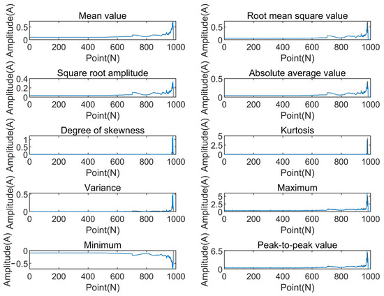
Figure 2.
Dimensional indicators of rolling bearings.
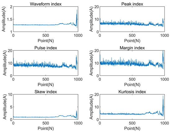
Figure 3.
Dimensionless indicators of rolling bearings.
From Figure 2 and Figure 3, it can be seen that the weight of various indicators in the whole life cycle of bearings is different, and the working conditions of bearings are also different. For example, the mean value and skewness in Figure 2 almost do not contain degradation characteristics, and kurtosis is not reflected until the bearing is almost invalid, which shows that they are extremely sensitive to early fault information. The dimensionless indicators’ peak index and pulse index in Figure 3 are poor in stability. Although they show some degradation information, the indicators are generally noisy and fluctuate greatly, so they should not be used as the deterioration performance indexes of bearings. Therefore, it is critical to find the indicators that can better capture this degradation trend and that are more sensitive to early failure.
3.2. Degradation Index
Extract the characteristic information of the selected dataset in the time-domain, frequency-domain and time-frequency domain, then use principal component analysis to reduce the dimension to obtain the degradation performance index, and select the first principal component. The results are shown in Figure 4.
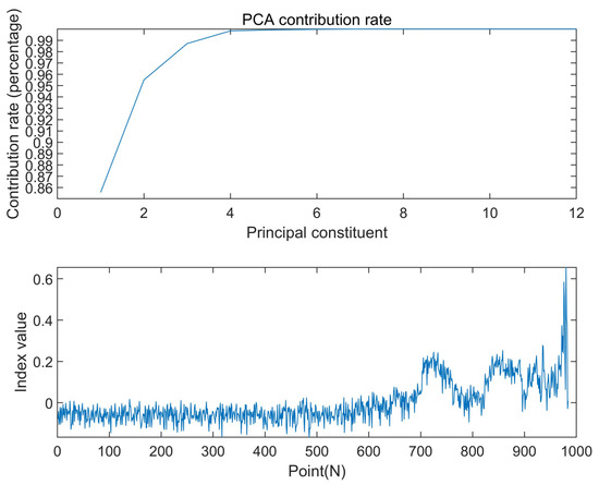
Figure 4.
PCA index of bearing life.
It can be seen from Figure 4 that the upward fluctuation begins at approximately 600 points, indicating that the bearing deterioration performance index obtained through PCA is more sensitive to the early fault information of the bearing. Compared with the single kurtosis index before dimension reduction, the overall stability of the kurtosis index is slightly poor, and it is not reflected until 750 points (Figure 3). The results show that using PCA to simplify the data can get a better performance degradation index over the whole life cycle of the bearing.
This indicator summarizes the degradation trend during the whole life of the bearing. It includes the whole process of rolling bearing vibration signal from the stable (normal) state in the early stage, to the early fault and the time when the later fault occurs. According to the previous analysis, one point represents 10 min. After conversion, when the rolling bearing testbed is operated for approximately 95 h, the performance index changes abruptly, indicating that the rolling bearing has a tendency towards early failure. The performance index rises steadily from 95 h to 117 h and changes abruptly at 117 h. From 117 h to 150 h, its performance index shows a serious shock trend. After 150 h, the change in its performance index is very irregular. At this time, the rolling bearing has a serious failure, which is just consistent with the experimental platform data.
According to the experimental method described in the previous section, the sample points of the whole life cycle of the PCA index set are divided equally into test set and training set at 1:1, and the whole life indexes of the test set and training set are shown in Figure 5 and Figure 6. The results show that the training group and the test group can still represent the whole life cycle, reducing the amount of calculation while maintaining a relatively complete bearing degradation information.
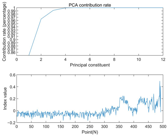
Figure 5.
PCA index of the training set.
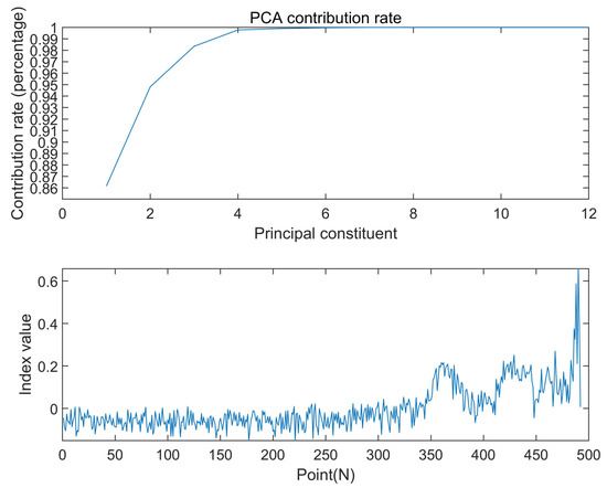
Figure 6.
PCA index of the test set.
3.3. Prediction Model
The best SVM parameters, C and g, for regression prediction analysis are C = 3.70986 and g = 0.249359, respectively. The iteration times are shown in Figure 7. The squirrel algorithm was used to obtain the actual and predicted values of the test set, as shown in Figure 8. The squirrel algorithm completed the optimization in the first twenty generations, and jumped out of local search many times, with a good convergence speed and a global search ability.
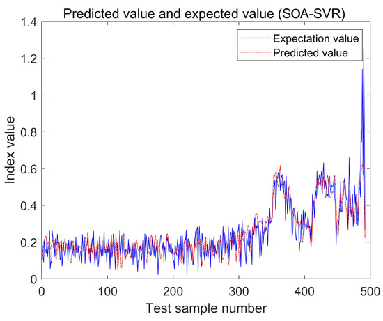
Figure 7.
The regression prediction analysis of the test set.
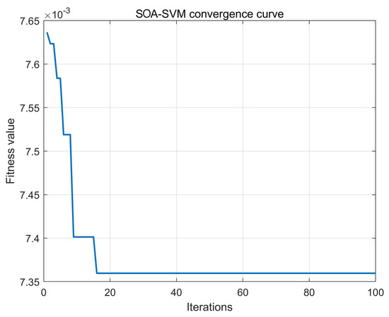
Figure 8.
The convergence curve of the test set.
From the prediction results, the first sudden change in the bearing occurred at 116.7 h (as shown in point 350 in Figure 8), which can be regarded as the early failure of the rolling bearing. From 116.7 h to 150 h (point 450 in Figure 8), the working index of the rolling bearing had obvious vibration, which can be judged as the medium failure period of the rolling bearing. Therefore, the prediction results well represented all stages of the bearing’s life cycle. In addition, the comparison with the test set also reflects the accuracy and practicality of the prediction results. It will effectively help engineers detect and maintain bearing equipment in advance.
In order to show the difference between the actual value and the predicted value more subtly, the error between the two was calculated and depicted in Figure 9. The average absolute error MAE is 0.057694, and the average percentage error MAPE is 33.8516%. The MAE can avoid the problem that errors cancel each other out, so it can accurately reflect the actual prediction error. In order to evaluate the prediction accuracy of the squirrel algorithm, evaluation indicators will be established in the next section.
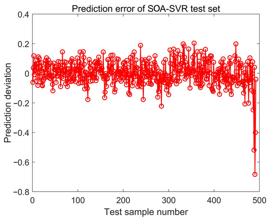
Figure 9.
The prediction error of the test set.
3.4. Evaluating Indicator
With the same population size and the maximum number of iterations, the SOA-SVM, GA-SVM and PSO-SVM algorithms were used to get the best solution, and root mean squared error (RMSE) and mean absolute error (MAE) were used as indicators [38] to compare and analyze the prediction ability. Using the genetic algorithm, training the same training set and verifying the test set, the best parameters, C = 158.477 and g = 0.340508, were obtained. The actual value and predicted value of the test set are shown in Figure 10, and the error diagram is shown in Figure 11. Using the particle swarm optimization algorithm, the best parameters, C = 89.8236 and g = 389.298, were obtained, and the actual value and predicted value of the test set are also printed out in Figure 12, and the error diagram is shown in Figure 13.
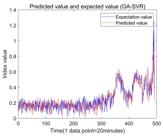
Figure 10.
The regression prediction analysis of the test set by GA-SVR.
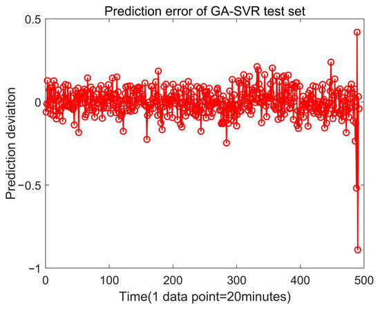
Figure 11.
The prediction error of the test set by GA-SVR.
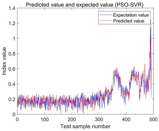
Figure 12.
The regression prediction analysis of the test set by PSO-SVR.
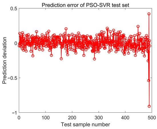
Figure 13.
The prediction error of the test set by PSO-SVR.
According to the prediction results of the PSO and the GA algorithms, both the PSO and GA algorithms completed the prediction of the test set, and there was an obvious upward trend at 116.7 h (point 350 in Figure 10 and Figure 12), which indicated that the bearing had an early failure tendency. From 116.7 h to 150 h (point 450 in Figure 10 and Figure 12), the working index of the rolling bearing had an obvious vibration, which can be judged as the medium failure period of the rolling bearing. This is basically consistent with previous research [39].
Finally, the grid search algorithm was used to train the same training set and verify the test set, and the best parameters, C = 0.1894 and g = 0.01184, were obtained. The actual and predicted values of the test set are shown in Figure 14, and the error diagram is shown in Figure 15.
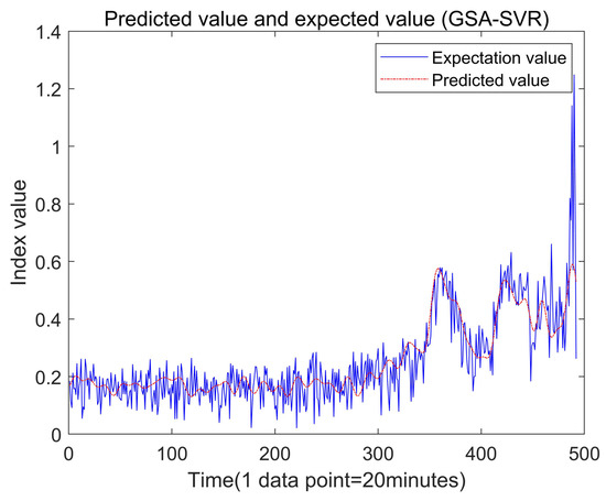
Figure 14.
The regression prediction analysis of the test set by GSA-SVR.
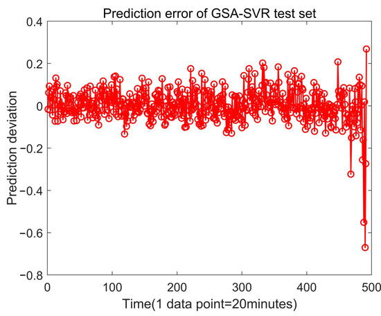
Figure 15.
The prediction error of the test set by GSA-SVR.
The evaluation indicators of the three algorithms are shown in Table 4. Compared with the GA-SVM, the PSO-SVM and the GSA-SVM algorithms, the SOA-SVM algorithm has greater advantages. By analyzing the values of MAE and RMSE, the SOA-SVM algorithm reduces the error by 5.1% and 13.6% compared with the GA-SVM algorithm. Compared with the PSO-SVM algorithm, the SOA-SVM algorithm reduces the error by 7.6% and 15.9%. It is worth mentioning that compared with the GSA-SVM algorithm, the error of the SOA algorithm is reduced by 8.4% and 16.3%, respectively.

Table 4.
The prediction error of the test set by different algorithms.
Based on the analysis of Figure 7, Figure 8, Figure 9, Figure 10, Figure 11, Figure 12, Figure 13, Figure 14 and Figure 15 and Table 4, it can be seen that the early, mild and moderate failures of rolling bearings can be effectively summarized by using the PCA method to fuse multi-dimensional datasets of time-domain features, which provides a data basis for the life prediction of rolling bearings. At the same time, combining SOA algorithms to optimize the kernel function parameters and penalty factors in SVM prediction models can effectively improve the regression accuracy and generalization ability of SVMs, so as to improve the prediction accuracy.
4. Discussion
In 2007, Huang et al. [40] successfully developed a practical life prediction model for ball bearings based on six vibration characteristics. In recent years, more and more studies have shown that the fusion of multi-dimensional eigenvectors can better represent the performance degradation of bearings, and that a single index has defects in representing the overall performance index. In this paper, we extracted the dimensional and non-dimensional indicators of bearings, and finally selected eleven indicators to represent the state indicators of bearings according to their actual performance, which were used in a later study on the decline process of bearings.
Then we used principal component analysis to simplify and reduce the dimensions of the selected features. We find that when we choose the appropriate characteristic indicators for fusion, the accuracy rate is obviously improved [41]. The state of life of the bearing can be intuitively reflected by a curve, so that relevant personnel can judge the state of the bearing more quickly and efficiently when monitoring its dynamic performance indicators. It provides a powerful tool for the maintenance and repair of the bearing.
After we have extracted the bearing degradation feature, we find that this feature can represent the full-cycle life of the bearing. In order to better help inspectors predict the remaining life of the bearing in advance, we adopted the support vector regression algorithm for prediction [42]. Squirrel optimization has shown good prediction ability in many fields since it was developed in 2019, so we proposed using the squirrel optimization algorithm to find the best kernel function parameters and penalty factors, and then apply them to the life prediction of bearings.
The prediction model we established successfully simulated the decline of the performance index of the bearing, and the desired prediction model of the remaining life of the bearing was obtained through SOA-SVM prediction. The model also includes the early failure, mid-failure and severe damage stages of the bearing. In the early stages of failure, the degradation index of the bearing rises rapidly, which indicates that the bearing has a failure tendency. Then, the predicted degradation index of the bearing vibrates violently, and the bearing enters the mid-term failure stage. The analysis shows that the degradation index of bearing performance is very sensitive to its damage, and will cause the bearing to have serious failure, which indicates that the prediction effect is good.
By fitting the bearing test set under the same working condition for each algorithm to get the optimal solution, compared with traditional prediction models, such as GA-SVM and PSO-SVM, the errors of SOA-SVM are slightly smaller, which means that the SOA-SVM proposed in this paper has greater advantages in predicting bearing life. However, when the dimension of the problem increases, the search space increases exponentially, and the data of the local optimal solution increases sharply, the algorithm may fall into a local optimal solution. Meanwhile, the possible population will stagnate at the local optimal solution, and the results may be different each time. Therefore, it will require more bearing data for verification in the future.
Since the publication of the Cincinnati full-cycle life dataset, a large number of scholars have used the dataset to study the full-cycle life of bearings [43]. One of the most important research directions is the estimation of the RUL of bearings based on the global meta-heuristic optimization algorithm. Zhao et al. [44] compared the RUL prediction results of the long-term and short-term memory (LSTM) neural network model with the support vector regression (SVR) by using the bearing life test data, and pointed out the shortcomings of the SVM regression prediction. However, in our study, we used the SOA algorithm to optimize the support vector regression prediction to further improve the accuracy of the SVM regression prediction. Yan et al. [45] defined five degradation stages and used the SVM classifier to evaluate the degradation stages of bearings. Due to its good generalization ability and mathematical foundation, it had high classification accuracy. Unfortunately, they did not adopt an optimization algorithm to improve the accuracy. However, SVM regression prediction combined with an SOA algorithm can provide some prediction data to classify and judge different degradation stages. Yan et al. [34] built an SVM prediction model by improving the optimized PSO algorithm to realize the bearing life prediction, but the prediction accuracy was lower than the SOA algorithm in this paper. However, there is no optimization algorithm that can be superior to all other algorithms in all scenarios [46]. At present, there are still many improvements in the application of an SOA algorithm in the field of bearing RUL prediction.
We have studied the relationship between the bearing time-domain characteristics and its life. Unfortunately, we have not entered into deep integration from other angles, such as frequency domain and time-frequency domain, to seek a better recession index. Some scholars have conducted relevant research in this respect. For example, Prost et al. [47] used time-frequency to analyze the remaining life of bearings. In addition, some scholars have optimized the squirrel algorithm to improve its search ability. RSOA is proposed to enhance the search ability of the squirrel algorithm, and its performance has been improved [48]. The SOA algorithm still has great room for improvement in global and local search capabilities, which is helpful to improve the accuracy and stability of the algorithm as much as possible with a limited number of iterations.
5. Conclusions
The comprehensive characteristic index can relatively accurately describe the fault information and bearing degradation process; however, it increases the computational complexity. In this paper, we proposed using PCA to synthesize multiple characteristic indexes to reduce the dimension and form a principal element with more characteristics. The new principal element was used as the degradation characteristic quantity of bearing life prediction to extract feature vectors. This method reduces the amount of calculation, while maintaining a more complete bearing degradation information. Finally, based on the optimized SVM, we used different algorithms to recognize the degraded features, and complete the life prediction of the bearing. The results showed that the bearing life prediction based on SOA-SVM is the best, which will play a good guiding role in the maintenance and detection of bearing equipment.
Author Contributions
Conceptualization, X.L. and Y.H.; methodology, X.L.; software, S.A.; validation, X.L., Y.S. and Y.H.; formal analysis, S.A.; investigation, X.L.; resources, X.L.; data curation, Y.S.; writing—original draft preparation, S.A.; writing—review and editing, X.L.; visualization, X.L.; supervision, X.L.; project administration, X.L.; funding acquisition, X.L. All authors have read and agreed to the published version of the manuscript.
Funding
This work was financially supported by the National Natural Science Foundation of China (NSFC), under grant no. 52005169.
Institutional Review Board Statement
Not applicable.
Informed Consent Statement
Not applicable.
Data Availability Statement
Data presented in this study are available in this article.
Acknowledgments
The authors acknowledge the financial support from the National Natural Science Foundation of China (grant no. 52005169).
Conflicts of Interest
The authors declare no conflict of interest.
References
- Si, X.S.; Wang, W.; Hu, C.H.; Zhou, D.H. Remaining useful life estimation–A review on the statistical data driven approaches. Eur. J. Oper. Res. 2011, 213, 1–14. [Google Scholar]
- Fuqing, Y.; Kumar, U. Statistical Index Development from Time Domain for Rolling Element Bearings. Int. J. Perform. Eng. 2014, 10, 1–8. [Google Scholar]
- Cao, H.; Niu, L.; Xi, S.; Chen, X. Mechanical model development of rolling bearing-rotor systems: A review. Mech. Syst. Signal Process. 2018, 102, 37–58. [Google Scholar]
- Cui, L.; Wang, X.; Xu, Y.; Jiang, H.; Zhou, J. A novel switching unscented Kalman filter method for remaining useful life prediction of rolling bearing. Measurement 2019, 135, 678–684. [Google Scholar] [CrossRef]
- Zhao, H.; Liu, H.; Jin, Y.; Dang, X.; Deng, W. Feature extraction for data-driven remaining useful life prediction of rolling bearings. IEEE Trans. Instrum. Meas. 2021, 70, 1–10. [Google Scholar] [CrossRef]
- Chang, H.; Yeung, D.Y. Robust locally linear embedding. Pattern Recognit. 2006, 39, 1053–1065. [Google Scholar] [CrossRef]
- Ding, S.; Qi, B.; Tan, H. A review of support vector machine theory and algorithm. J. Univ. Electron. Sci. Technol. 2011, 40, 2–10. [Google Scholar]
- Şentaş, A.; Tashiev, İ.; Küçükayvaz, F.; Kul, S.; Eken, S.; Sayar, A.; Becerikli, Y. Performance evaluation of support vector machine and convolutional neural network algorithms in real-time vehicle type and color classification. Evol. Intell. 2020, 13, 83–91. [Google Scholar] [CrossRef]
- Sun, C.; Zhang, Z.; He, Z. Research on bearing life prediction based on support vector machine and its application. J. Phys. Conf. Ser. 2011, 305, 012028. [Google Scholar] [CrossRef]
- Zhao, F.; Chen, J.; Xu, W. Condition prediction based on wavelet packet transform and least squares support vector machine methods. Proc. Inst. Mech. Eng. Part E J. Process Mech. Eng. 2009, 223, 71–79. [Google Scholar] [CrossRef]
- Chen, Z.; Cao, S.; Mao, Z. Remaining useful life estimation of aircraft engines using a modified similarity and supporting vector machine (SVM) approach. Energies 2017, 11, 28. [Google Scholar] [CrossRef]
- Bao, W.; Wang, H.; Chen, J.; Zhang, B.; Ding, P.; Wu, J.; He, P. Life prediction of slewing bearing based on isometric mapping and fuzzy support vector regression. Trans. Inst. Meas. Control 2020, 42, 94–103. [Google Scholar] [CrossRef]
- Huang, C.L.; Wang, C.J. A GA-based feature selection and parameters optimizationfor support vector machines. Expert Syst. Appl. 2006, 31, 231–240. [Google Scholar] [CrossRef]
- Feng, Z.K.; Niu, W.J.; Tang, Z.Y.; Jiang, Z.Q.; Xu, Y.; Liu, Y.; Zhang, H.R. Monthly runoff time series prediction by variational mode decomposition and support vector machine based on quantum-behaved particle swarm optimization. J. Hydrol. 2020, 583, 124627. [Google Scholar] [CrossRef]
- Guermoui, M.; Gairaa, K.; Boland, J.; Arrif, T. A novel hybrid model for solar radiation forecasting using support vector machine and bee colony optimization algorithm: Review and case study. J. Sol. Energy Eng. 2021, 143, 1–10. [Google Scholar] [CrossRef]
- Xue, J.; Shen, B. A novel swarm intelligence optimization approach: Sparrow search algorithm. Syst. Sci. Control Eng. 2020, 8, 22–34. [Google Scholar] [CrossRef]
- Dong, J.; Dou, Z.; Si, S.; Wang, Z.; Liu, L. Optimization of capacity configuration of wind–solar–diesel–storage using improved sparrow search algorithm. J. Electr. Eng. Technol. 2022, 17, 1–14. [Google Scholar] [CrossRef]
- Jianhua, L.; Zhiheng, W. A hybrid sparrow search algorithm based on constructing similarity. IEEE Access 2021, 9, 117581–117595. [Google Scholar] [CrossRef]
- Zhang, C.; Ding, S. A stochastic configuration network based on chaotic sparrow search algorithm. Knowl.-Based Syst. 2021, 220, 106924. [Google Scholar] [CrossRef]
- Sörensen, K.; Glover, F. Metaheuristics. Encycl. Oper. Res. Manag. Sci. 2013, 62, 960–970. [Google Scholar]
- Qiu, G.; Gu, Y.; Chen, J. Selective health indicator for bearings ensemble remaining useful life prediction with genetic algorithm and Weibull proportional hazards model. Measurement 2020, 150, 107097. [Google Scholar] [CrossRef]
- Souto, M.C.B.; das Chagas MourA, M.; Lins, I.D. Particle swarm-optimized support vector machines and pre-processing techniques for remaining useful life estimation of bearings. Eksploat. I Niezawodn. 2019, 21, 610–618. [Google Scholar]
- Cheng, Y.; Hu, K.; Wu, J.; Zhu, H.; Lee, C.K. A deep learning-based two-stage prognostic approach for remaining useful life of rolling bearing. Appl. Intell. 2022, 52, 5880–5895. [Google Scholar] [CrossRef]
- Pan, Y.; Cheng, D.; Wei, T.; Jia, Y. Rolling bearing performance degradation assessment based on deep belief network and improved support vector data description. Mech. Syst. Signal Process. 2022, 181, 109458. [Google Scholar] [CrossRef]
- Jain, M.; Singh, V.; Rani, A. A novel nature-inspired algorithm for optimization: Squirrel search algorithm. Swarm Evol. Comput. 2019, 44, 148–175. [Google Scholar] [CrossRef]
- Khare, A.; Agrawal, S. Scheduling hybrid flowshop with sequence-dependent setup times and due windows to minimize total weighted earliness and tardiness. Comput. Ind. Eng. 2019, 135, 780–792. [Google Scholar]
- Sakthivel, V.; Suman, M.; Sathya, P. Squirrel search algorithm for economic dispatch with valve-point effects and multiple fuels. Energy Sources Part B Econ. Plan. Policy 2020, 15, 351–382. [Google Scholar] [CrossRef]
- Basu, M. Squirrel search algorithm for multi-region combined heat and power economic dispatch incorporating renewable energy sources. Energy 2019, 182, 296–305. [Google Scholar] [CrossRef]
- Yu, J. Bearing performance degradation assessment using locality preserving projections and Gaussian mixture models. Mech. Syst. Signal Process. 2011, 25, 2573–2588. [Google Scholar] [CrossRef]
- Lee, J.; Qiu, H.; Yu, G.; Lin, J. Rexnord Technical Services: Bearing Data Set. IMS, University of Cincinnati. “Bearing Data Set”, NASA Prognostics Data Repository; NASA Ames Research Center: Moffett Field, CA, USA, 2007. Available online: https://www.nasa.gov/content/prognostics-center-of-excellence-data-set-repository (accessed on 22 June 2022).
- Kashef, R. A boosted SVM classifier trained by incremental learning and decremental unlearning approach. Expert Syst. Appl. 2021, 167, 114154. [Google Scholar] [CrossRef]
- Liu, W.; Chen, F.; Chen, Y. PM2.5 Concentration Prediction Based on Pollutant Pattern Recognition Using PCA-clustering Method and CS Algorithm Optimized SVR. Nat. Environ. Pollut. Technol. 2022, 21, 393–403. [Google Scholar] [CrossRef]
- Garcia-Gonzalo, E.; Fernandez-Martinez, J.L. A brief historical review of particle swarm optimization (PSO). J. Bioinform. Intell. Control 2012, 1, 3–16. [Google Scholar] [CrossRef]
- Zhang, Y.; Tang, B.; Xiong, P. Rolling element bearing life prediction based on multi-scale mutation particle swarm optimized multi-kernel least square support vector machine. Chin. J. Sci. Instrum. 2016, 37, 2489–2496. [Google Scholar]
- Shi, Y.; Eberhart, R. A modified particle swarm optimizer. In Proceedings of the 1998 IEEE International Conference on Evolutionary Computation Proceedings. IEEE World Congress on Computational Intelligence (Cat. No. 98TH8360), Anchorage, AK, USA, 4–9 May 1998; pp. 69–73. [Google Scholar]
- Basharat, S.; Jain, S. Studying Genetic Algorithm and Particle Swarm Optimization In Machine Learning. ICIDSSD 2021, 2020, 81. [Google Scholar]
- Al-Azzawi, D.S. Evaluation of Genetic Algorithm Optimization in Machine Learning. J. Inf. Sci. Eng. 2020, 36, 231–241. [Google Scholar]
- Wang, W.; Lu, Y. Analysis of the mean absolute error (MAE) and the root mean square error (RMSE) in assessing rounding model. IOP Conf. Ser. Mater. Sci. Eng. 2018, 324, 012049. [Google Scholar] [CrossRef]
- Nieto, P.G.; García-Gonzalo, E.; Lasheras, F.S.; de Cos Juez, F.J. Hybrid PSO–SVM-based method for forecasting of the remaining useful life for aircraft engines and evaluation of its reliability. Reliab. Eng. Syst. Saf. 2015, 138, 219–231. [Google Scholar] [CrossRef]
- Huang, R.; Xi, L.; Li, X.; Liu, C.R.; Qiu, H.; Lee, J. Residual life predictions for ball bearings based on self-organizing map and back propagation neural network methods. Mech. Syst. Signal Process. 2007, 21, 193–207. [Google Scholar] [CrossRef]
- Yan, J.; Guo, C.; Wang, X. A dynamic multi-scale Markov model based methodology for remaining life prediction. Mech. Syst. Signal Process. 2011, 25, 1364–1376. [Google Scholar] [CrossRef]
- Borthakur, N.; Dey, A.K. Evaluation of group capacity of micropile in soft clayey soil from experimental analysis using SVM-based prediction model. Int. J. Geomech. 2020, 20, 04020008. [Google Scholar] [CrossRef]
- Gousseau, W.; Antoni, J.; Girardin, F.; Griffaton, J. Analysis of the Rolling Element Bearing data set of the Center for Intelligent Maintenance Systems of the University of Cincinnati. In Proceedings of the CM2016, Shenzhen, China, 11–13 November 2016. [Google Scholar]
- Zhai, Y.; Deng, A.; Li, J.; Cheng, Q.; Ren, W. Remaining Useful Life Prediction of Rolling Bearings Based on Recurrent Neural Network. J. Artif. Intell. 2019, 1, 19. [Google Scholar] [CrossRef]
- Yan, M.; Wang, X.; Wang, B.; Chang, M.; Muhammad, I. Bearing remaining useful life prediction using support vector machine and hybrid degradation tracking model. ISA Trans. 2020, 98, 471–482. [Google Scholar] [CrossRef] [PubMed]
- Wolpert, D.H.; Macready, W.G. No free lunch theorems for optimization. IEEE Trans. Evol. Comput. 1997, 1, 67–82. [Google Scholar] [CrossRef]
- Prost, J.; Boidi, G.; Varga, M.; Vorlaufer, G.; Eder, S. Lifetime assessment of porous journal bearings using joint time-frequency analysis of real-time sensor data. Tribol. Int. 2022, 169, 107488. [Google Scholar] [CrossRef]
- Zhang, X.; Zhao, K.; Wang, L.; Wang, Y.; Niu, Y. An improved squirrel search algorithm with reproductive behavior. IEEE Access 2020, 8, 101118–101132. [Google Scholar] [CrossRef]
Publisher’s Note: MDPI stays neutral with regard to jurisdictional claims in published maps and institutional affiliations. |
© 2022 by the authors. Licensee MDPI, Basel, Switzerland. This article is an open access article distributed under the terms and conditions of the Creative Commons Attribution (CC BY) license (https://creativecommons.org/licenses/by/4.0/).