Friction Prediction and Application to Lateral or Longitudinal Slip Force Prediction

Abstract

The empirical or semi-empirical model is widely used for vehicle simulation because of its high accuracy but relies on massive experimental data of tire force and moment. Therefore, tire mechanical prediction is of great significance to improve tire modeling efficiency and to reduce costs. Typical prediction methods or models based on normalization presented by Pacejka and Radt assume that different loads could be close to one normalized curve, but it is not always accurate enough to predict tire force under pure slip conditions and there is no mention of friction prediction methods. In the paper, a theoretical model considering the deformation of belt/carcass is established, which lays the foundation for a normalization model. A method for separation of friction from test data and the proportional assumption of longitudinal and lateral peak friction coefficient between target tire and reference tire are proposed, and the experimental results show that this assumption is acceptable. Finally, according to the separation of friction method and assumption, a new prediction method for tire force under pure slip conditions is presented and validated by comparison with the experimental data. It shows that the proposed method has good prediction capability with satisfactory accuracy.

1. Introduction

The empirical or semi-empirical is always used for vehicle dynamics and its model parameters are obtained by fitting measurements, which relies on massive experimental data, including MF/PAC2002 [1,2,3,4], TMeasy [5,6,7], UniTire [8,9], Hankook-Tire [10], TameTire [11,12], MF-Swift [13,14], FTire [15,16], CDTire [17,18] and RMOD-K [19,20] model, etc. Compared with the pure cornering force, it is more difficult to obtain the longitudinal slip characteristic for the torque limit of a tire test rig [21], which brings serious challenges to the measurement of large-sized tires represented by electric vehicle tires. Therefore, if there is a method that can realize the prediction of pure longitudinal or pure lateral slip force, it is of great significance to improve tire modeling efficiency and reduce test costs and it can also make up for the lack of longitudinal force measurement ability.

Measurement for testing tire characteristics can be divided into two categories: an indoor test, including typical low-speed flat plank, high-speed flat track, and inner/outer drum test; and an outdoor test by using the Tire Test Trailer or on-vehicle test with six-component force/torque transducer directly [22]. Additionally, different road conditions and speeds usually lead to different friction coefficients and slip stiffness [23,24,25,26,27,28,29,30], which have significant influence on tire mechanical properties. For example, the friction coefficient of indoor test machines is usually larger than that of outdoor road conditions [24,25]. Therefore, how to achieve friction separation through indoor test data? Insertion of different friction coefficients is realized through the indoor friction test, and the tire characteristics under different friction are obtained, which is important for the design and analysis of vehicle dynamics and active safety systems [22] since different studies have developed and used different algorithms to estimate the tire-road friction. Based on the approaches that they have followed, all of the related research can be divided into the following two categories: experiment-based and model-based [31]. In experiment-based approaches, it is attempted to find a correlation between the sensor data (acoustic sensors, temperature sensor, etc.) and tire-road friction related parameters [31,32,33,34,35,36,37]. The model-based approaches try to estimate the friction using simplified mathematical models, which can be divided into three sub-categories: wheel and vehicle dynamic based approaches, slip based approaches, and tire model based approaches [29,38,39,40,41,42]. It is also necessary to analyze the contact of tires with the test stand and to recognize the slip conditions on dynamometric stands [43].

According to tire dynamics theory and previous studies, the two keys to pure condition prediction are normalized curve or nondimensionalization of tire characteristics and dynamic friction. Pacejka proposed the Similarity method based on the normalization theory of the Fiala model [2,44]. A demonstration that, in practice, similarity indeed approximately occurs is given by Radt and Milliken [44,45]; several tires dimensionless plots are shown, and it is found that most of the side force data at different loads can be made to fall on a single dimensionless curve as a function of combined steer and camber angle ratios, provided the camber angle does not exceed 10 degrees. Similarly, it is shown that dimensionless braking force at various loads becomes a single curve as a function of the slip ratio parameter for zero steer angle, and as a function of the steer angle parameter for constant values of the slip ratio parameter [44,45]. Kasprzak, E. M et al. eliminate tire asymmetries in lateral and longitudinal force by using “zero-offset data”, the friction coefficients are determined independently for the left and right sides, and the influence of inflation pressure is taken into account in the dimensionless model [46,47]. These important findings lay a foundation for the prediction of tire mechanical properties. However, in the process of normalization, since the peak friction coefficient is used for normalization, dynamic friction separation is not achieved, which will result in a difference in the normalized curve in the transition region. Because the load will affect the pressure distribution of the contact patch, it will also lead to the difference of the transition region from the normalized curve. Therefore, it is not reasonable to consider the normalized curve under different loads as the same, and the tire specifications studied at the time were generally small which affected the applicability of the conclusions.

R.S. and Bettella, M. explores the possibility of predicting tire mechanical properties based on minimum test data or the basic sets and similarity ideas are used in association with the “Magic Formula”. Advantages are obtained by using a novel nonlinear slip transformation of the longitudinal and sideslip variables. The results are shown to be qualitatively excellent and quantitatively quite good. Of course, the accuracy is not as high as with a full Magic Formula treatment, but the economy is remarkable [48,49,50]. However, because the magic formula cannot express the separation of dynamic friction, the nonlinear transformation becomes complicated and the transformation accuracy is reduced.

The UniTire model realizes the separation of dynamic friction and normalization of dimensionless shear force and has a good basis for prediction [8,9]. In the application of the UniTire model, the friction coefficient is identified together with the normalized curve, which leads to dynamic friction deviation between model and test and so it cannot reflect the normalized curve of the actual tire. Nan Xu et al. [22] give a data-driven tire capacity estimation method based on $\overline{F}~S$ relationship using UniTire, but $\overline{F}$ is obtained similar to Radt and Milliken [44,45], which will also cause similar problems.

This paper proposes a simple method for dynamic friction separation from the larger slip condition, and the pure sideslip and pure longitudinal slip of different tires are normalized according to loads. Experimental results show that the proposed dynamic friction separation method makes the normalized curves highly coincident under a similar load condition. It is found that under similar load conditions, the ratio of lateral and longitudinal peak friction coefficients of different tires is approximately equal and the proportional relation hypothesis of lateral and longitudinal dynamic friction satisfying peak friction coefficient is proposed. The test results show that the hypothesis is reasonable. Finally, there is a new prediction model for pure longitudinal force or pure lateral force based on normalization results by using reference tire and dynamics friction prediction. It shows the prediction results of longitudinal force or lateral force are in good agreement with the experimental data.

2. Method of Dynamic Friction Prediction

2.1. Peak Friction Coefficient Assumption and Validation

According to the observation of the tire force measurements of the passenger tire, the ratio of the longitudinal peak friction coefficient to the lateral peak friction coefficient of the reference tire and the target tire is relatively stable under a similar test condition. Especially considering tire size, tread pattern and compound, and test sequence.

In order to verify the hypothesis of the proportional relationship between the longitudinal and lateral peak friction coefficient of the reference tire and the target tire. Four groups of passenger car tires were selected, as shown in

Table 1. Tire groups and basic information.

Group	Tire Size	Tire No.	Pressure [kPa]	Tread Depth [mm]
(1) Same tire mold and tread compound, different structural design	205/55R16-P1-C1-T1	1	230	6.8
	205/55R16-P1-C1-T2	2	230	6.8
(2) Same tire mold, different tread compound and structural design	205/55R16-P1-C1-T1	3	230	6.8
	205/55R16-P1-C2-T3	4	230	6.8
(3) Same tire pattern, different size, tread compound and structural design	215/55R18-P2-C3-T4	5	250	7.6
	215/60R17-P2-C4-T5	6	250	7.2
(4) Different size with different tire manufacturer	195/55R16-P3-C5-T6	7	225	7.3
	215/60R17-P4-C6-T7	8	245	7.2

. The test speed was 60 km/h. All tire force tests were conducted on the MTS Flat-trac machine, as shown in Figure 1.

The four control groups were analyzed, and the longitudinal peak friction coefficient and lateral peak friction coefficient of these tires were extracted, respectively, as shown in

Table 2. The friction on the side of negative slip velocity.

Tire No.	${\mathit{\mu }}_{\mathit{x}\mathit{m}\mathit{a}\mathit{x}}$			${\mathit{\mu }}_{\mathit{y}\mathit{m}\mathit{a}\mathit{x}}$			${\mathit{\mu }}_{\mathit{x}\mathit{m}\mathit{a}\mathit{x}}/{\mathit{\mu }}_{\mathit{y}\mathit{m}\mathit{a}\mathit{x}}$
	${\mathit{F}}_{\mathit{z}1}$	${\mathit{F}}_{\mathit{z}2}$	${\mathit{F}}_{\mathit{z}3}$	${\mathit{F}}_{\mathit{z}1}$	${\mathit{F}}_{\mathit{z}2}$	${\mathit{F}}_{\mathit{z}3}$	${\mathit{F}}_{\mathit{z}1}$	${\mathit{F}}_{\mathit{z}2}$	${\mathit{F}}_{\mathit{z}3}$
1	1.19	1.18	1.11	1.19	1.06	0.97	1.00	1.11	1.14
2	1.18	1.17	1.11	1.19	1.06	0.97	0.99	1.11	1.15
3	1.19	1.18	1.11	1.19	1.06	0.97	1.00	1.11	1.14
4	1.15	1.16	1.16	1.11	1.04	0.96	1.03	1.12	1.21
5	1.24	1.20	1.16	1.19	1.08	1.00	1.04	1.11	1.16
6	1.27	1.22	1.14	1.23	1.13	1.01	1.03	1.08	1.13
7	1.20	1.17	1.15	1.16	1.02	0.95	1.04	1.14	1.21
8	1.17	1.15	1.13	1.08	1.07	0.94	1.09	1.08	1.20

and

Table 3. The friction on the side of positive slip velocity.

Tire No.	${\mathit{\mu }}_{\mathit{x}\mathit{m}\mathit{i}\mathit{n}}$			${\mathit{\mu }}_{\mathit{y}\mathit{m}\mathit{i}\mathit{n}}$			${\mathit{\mu }}_{\mathit{x}\mathit{m}\mathit{i}\mathit{n}}/{\mathit{\mu }}_{\mathit{y}\mathit{m}\mathit{i}\mathit{n}}$
	${\mathit{F}}_{\mathit{z}1}$	${\mathit{F}}_{\mathit{z}2}$	${\mathit{F}}_{\mathit{z}3}$	${\mathit{F}}_{\mathit{z}1}$	${\mathit{F}}_{\mathit{z}2}$	${\mathit{F}}_{\mathit{z}3}$	${\mathit{F}}_{\mathit{z}1}$	${\mathit{F}}_{\mathit{z}2}$	${\mathit{F}}_{\mathit{z}3}$
1	−1.27	−1.18	−1.06	−1.21	−1.04	−0.96	1.05	1.13	1.10
2	−1.26	−1.16	−1.06	−1.21	−1.03	−0.96	1.05	1.13	1.10
3	−1.27	−1.18	−1.06	−1.21	−1.04	−0.96	1.05	1.13	1.10
4	−1.12	−1.10	−1.15	−1.16	−1.04	−0.94	0.96	1.05	1.23
5	−1.10	−1.12	−1.11	−1.18	−1.08	−1.02	0.93	1.04	1.09
6	−1.19	−1.13	−1.05	−1.25	−1.13	−1.00	0.95	0.99	1.06
7	−1.14	−1.12	−1.12	−1.12	−1.00	−0.92	1.02	1.12	1.22
8	−1.12	−1.15	−1.14	−1.09	−1.02	−0.89	1.02	1.13	1.28

. For the convenience of calculation and comparison, the longitudinal force curve is mirrored on the Y-axis to convert to the same quadrant as the lateral force curve under ISO tire coordinate system.

The uppercase letters in table P represents the pattern type, C represents the compound type, and T represents the structural design type.

Therefore, the following assumptions are made for the longitudinal and lateral peak friction coefficients between the reference tire and the target tire.

$$\frac{{\mu }_{xpeak-ref}}{{\mu }_{ypeak-ref}}\approx \frac{{\mu }_{xpeak-pre}}{{\mu }_{ypeak-pre}}$$

(1)

where the ${\mu }_{xpeak-ref}$ and ${\mu }_{ypeak-ref}$ are the longitudinal and lateral peak friction coefficient of the reference tire, and the ${\mu }_{xpeak-pre}$ and ${\mu }_{ypeak-pre}$ are the longitudinal and lateral peak friction coefficient of the target tire. The target tire refers to the tire to predict the tire force, and the reference tire refers to the tire used as a reference in the prediction process of the target tire.

Figure 2 shows the ratio of the longitudinal and lateral peak friction coefficients of these four tire groups.

According to the above results, the assumption of the longitudinal and lateral peak friction coefficients of the target tire and the reference tire is satisfactory. If the reference tire is further classified, such as tire specification, tread pattern and compound, and test conditions, the friction prediction result is more reliable.

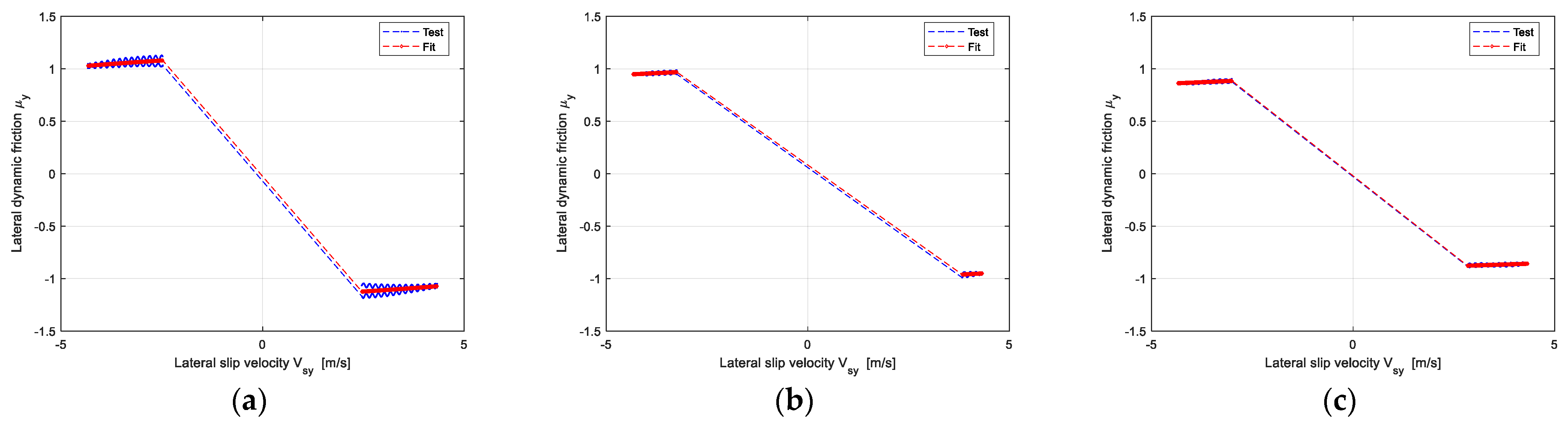
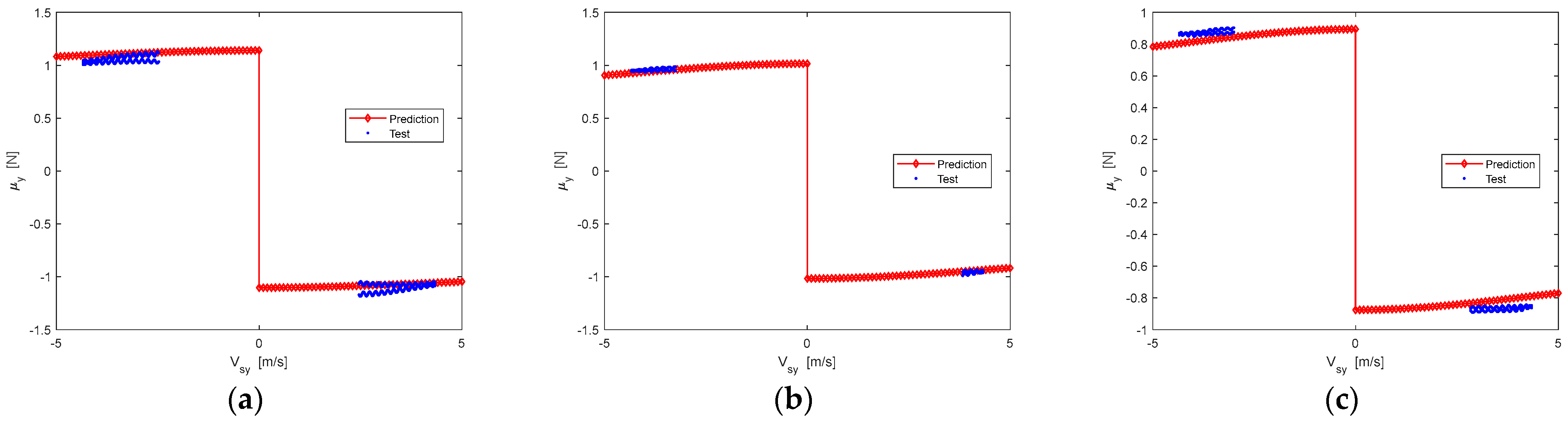
2.2. Dynamic Friction Separation Method

The friction is considered separately in the UniTire tire model, where the longitudinal and lateral friction can be expressed as [51,52]:

$$\{\begin{array}{l}{\mu }_x=\left({\mu }_{x0}-d{\mu }_{x0}\right)+d{\mu }_{x0}\cdot \mathrm{sech}\left(\frac{V_{sx}}{V_{smx}}\right)\\ {\mu }_y=\left({\mu }_{y0}-d{\mu }_{y0}\right)+d{\mu }_{y0}\cdot \mathrm{sech}\left(\frac{V_{sy}}{V_{smy}}\right)\end{array}$$

(2)

where ${\mu }_{x0}$, $d{\mu }_{x0}$ and $V_{smx}$ are longitudinal parameters, and ${\mu }_{y0}$, $d{\mu }_{y0}$ and $V_{smy}$ are lateral parameters of the friction model.

From the analysis of the theoretical model, it can be seen that the tire mechanical properties are only related to the dynamic friction because the value of dimensionless longitudinal force or dimensionless lateral force is 1 under the large slip condition. Therefore, the tire forces under large slip conditions were selected and fitted by Equation (2) to establish an empirical model of dynamic friction coefficient with slip velocity. So, the longitudinal and lateral peak friction coefficients under the corresponding load can be easily obtained. Thus, the separation of dynamic friction is realized.

Take Group 3 as an example; it has more challenges than Group 1 and Group 2. The passenger tire of 215/55R18 was selected as the reference tire to predict the target tire of 215/60R17. After measuring the pure cornering and pure braking/driving force of the two tires, the longitudinal and lateral friction coefficients under large slip conditions can be obtained according to Equation (2). The identification results of longitudinal and lateral dynamic friction of the reference tire are shown in Figure 3 and Figure 4.

The identification results of longitudinal and lateral dynamic friction of the target tire are shown in Figure 5 and Figure 6.

From the identification results of longitudinal and lateral dynamic friction, the expression of dynamic friction is reasonable with a very small error. Moreover, dynamic friction curves with the sliding velocity of the two tires are very similar under similar load conditions.

The peak friction coefficient is scaled to predict the dynamic friction under the other slip velocity. Therefore, the longitudinal and lateral dynamic friction can be expressed as:

$$\{\begin{array}{l}{\mu }_x=\frac{{\mu }_{ypeak-pre}}{{\mu }_{ypeak-ref}}\cdot {\mu }_{x-ref}\\ {\mu }_y=\frac{{\mu }_{xpeak-pre}}{{\mu }_{xpeak-ref}}\cdot {\mu }_{y-ref}\end{array}$$

(3)

where the ${\mu }_{x-ref}$ and ${\mu }_{y-ref}$ are the longitudinal and the lateral dynamic friction of the target tire, and the ${\mu }_x$ and ${\mu }_y$ are the longitudinal and the lateral dynamic friction of the reference tire.

According to Equation (1), the longitudinal peak friction coefficient of the target tire is obtained by using the pure cornering and pure braking/driving test data of the reference tire and pure cornering test data of target tire. Then, the longitudinal friction at different slip velocity can be acquired by Equation (3). The prediction results are shown in Figure 7 and Figure 8.

It can be seen that the prediction results of longitudinal or lateral friction have a little difference compared to the experimental data, but the overall prediction result is still satisfactory. Interestingly, the advantage of this prediction method is to achieve mutual prediction between longitudinal friction and lateral friction. If one of the friction characteristics is measured, the other friction can be predicted efficiently.

3. Prediction Method for Tire Forces under Pure Slip Condition

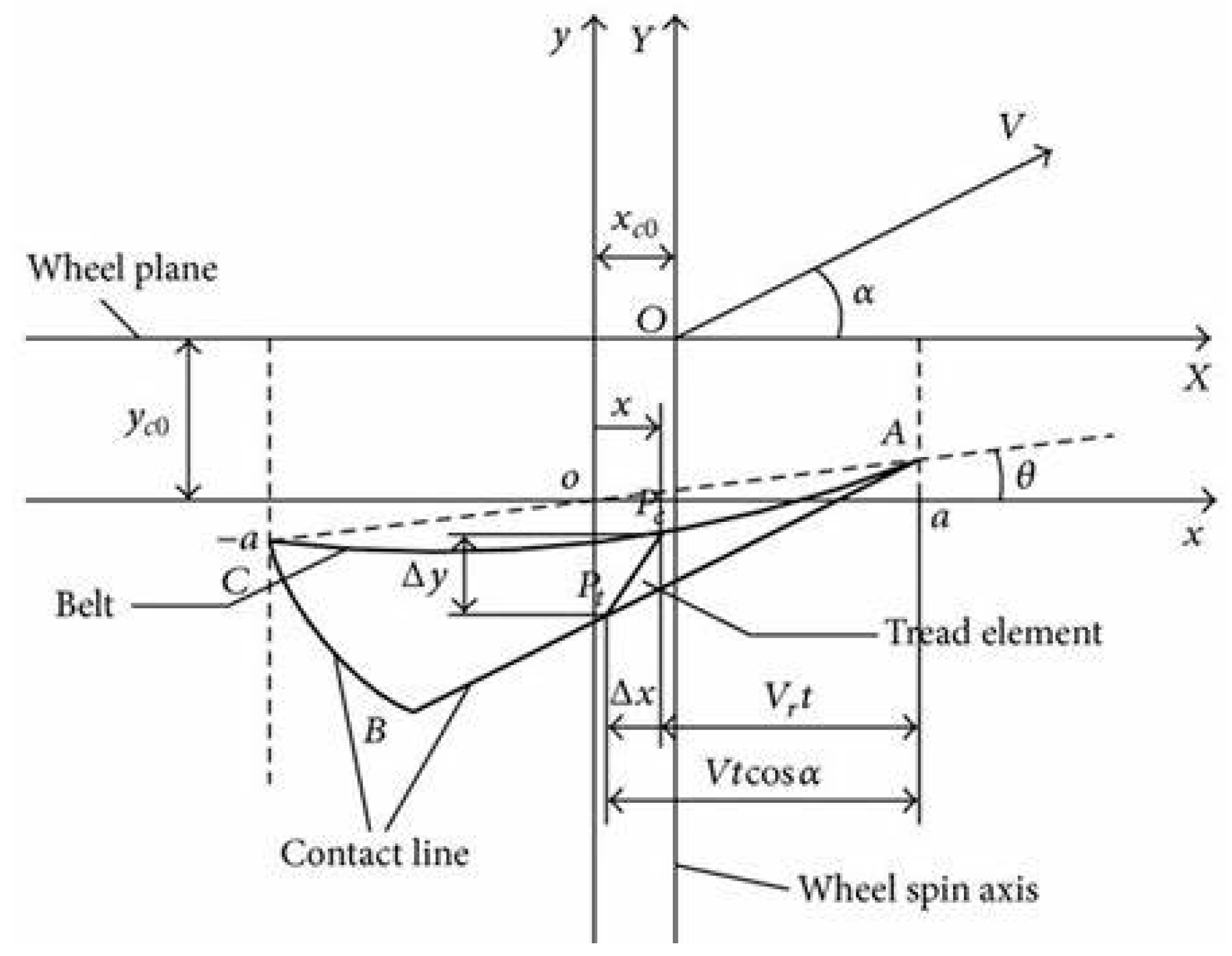
3.1. Theoretical Tire Model of Considering Belt/carcass Deformation

The deformation of belt/carcass and tread element of the physical tire model considering belt/carcass elasticity is shown in Figure 9 under the combined braking/driving and cornering conditions [53,54,55]. The relationship between tire force and motion input is shown in the Figure 9.

In this figure, $XOY$ is the tire axis system, $xoy$ is a relative coordinate system for describing the tread deformation with respect to the carcass. $V$ is the relative speed of the wheel center and the ground when the wheel rolls forward, $\alpha$. is slip angle, $a$ is half the length of the footprint.

‘ABC’ is the central line of the contact patch under combined slip condition. The whole length of contact patch $2a$ is divided into two parts, the adhesion region ‘AB’, and the sliding region ‘BC’, by the initial sliding point ‘B’. The $x_{c0}$ and $y_{c0}$ are longitudinal and lateral translational deformation of the carcass under combined longitudinal and lateral slip condition.

The tire deformation in the adhesion area can be calculated as:

$$\{\begin{array}{l}\Delta x=x_{pt}-x_{pc}=\left(a-x\right)\cdot S_x\\ \Delta y=y_{pt}-y_{pc}=\left(a-x\right)\cdot \left(\lambda S_y\right)\\ \Delta s=\sqrt{\Delta x^2+\Delta y^2}\end{array}$$

(4)

where $S_x$ is the longitudinal slip ratio, and $S_y$ is the lateral slip ratio in the model. The slip ratios are defined as the sliding speed over the rolling speed, as shown below.

$$\{\begin{array}{l}{S}_x=\frac{-V_{sx}}{V_r}=-\frac{V\cos \alpha -\mathsf{\Omega }{R}_e}{\mathsf{\Omega }{R}_e},S_x\in (-\infty ,\infty )\\ S_y=\frac{-V_{sy}}{V_r}=-\frac{V\sin \alpha }{\mathsf{\Omega }{R}_e},S_y\in (-\infty ,\infty )\end{array}$$

(5)

where $\mathsf{\Omega }$ is the rolling angular speed, $V_{sx}$ and $V_{sy}$ is the longitudinal and lateral slip velocity to the road surface, $V_r$ is the rolling velocity, $V$ is the wheel velocity, $\alpha$ is the slip angle, and $R_e$ is the effective rolling radius.

Then, the shear stress in both directions can be expressed as:

$$\{\begin{array}{l}{q}_{ax}=q\cdot \cos {\theta }_{qa}=\left(k_t\cdot \Delta s\right)\cdot \frac{\Delta x}{\Delta s}\\ q_{ay}=q\cdot \sin {\theta }_{qa}=\left(k_t\cdot \Delta s\right)\cdot \frac{\Delta y}{\Delta s}\end{array}$$

(6)

According to $q_a=q_s$ to determine the point of transition from adhesion to sliding region.

$$k\cdot \sqrt{\Delta x^2+\Delta y^2}={\mu }_0\cdot q_z$$

(7)

Because the lateral force and longitudinal force satisfy the elliptic relationship. Therefore, the following formula can be deduced:

$$\sqrt{{\left(\frac{K_x{S}_x}{{\mu }_{xo}\cdot F_z}\right)}^2+{\left(\frac{K_y{S}_y}{{\mu }_{yo}\cdot F_z}\right)}^2}=\sqrt{{\varphi }_x^2+{\varphi }_y^2}=\varphi =\frac{\eta \left(u_c\right)}{1-u_c}$$

(8)

where ${\varphi }_x$ is normalized longitudinal slip ratio, ${\varphi }_y$ is normalized lateral slip ratio, $\varphi$ is normalized combined slip ratio, $u_c$ is the point of transition from adhesion to sliding region, and $\eta \left(u_c\right)$ is normalized pressure distribution function. $K_x=2a^2{k}_t$, $K_y=\lambda ·2a^2{k}_t$ represent the longitudinal slip stiffness and cornering stiffness. a is half footprint length, k_t is brush distribution stiffness, and λ is anisotropic stiffness coefficient.

The normalized longitudinal slip ratio ${\varphi }_x$, lateral slip ratio ${\varphi }_y$, and combined slip ratio $\varphi$ are defined as:

$$\{\begin{array}{l}{\varphi }_x=\frac{K_x{S}_x}{{\mu }_{xo}\cdot F_z}\\ {\varphi }_y=\frac{K_y{S}_y}{{\mu }_{yo}\cdot F_z}\\ \varphi =\sqrt{{\varphi }_x^2+{\varphi }_y^2}\end{array}$$

(9)

According to the friction ellipse concept, it is defined as:

$$\sqrt{{\left({\mu }_{xo}\frac{{\varphi }_x}{\varphi }\right)}^2+{\left({\mu }_{yo}\frac{{\varphi }_y}{\varphi }\right)}^2}={\mu }_o$$

(10)

Finally, the expression of longitudinal force and lateral force under combined slip conditions can be derived as follows:

$$\begin{array}{l}\{\begin{array}{l}{F}_x={\displaystyle {\int }_{x_c}^a{q}_{ax}dx}+{\displaystyle {\int }_{-a}^{x_c}\frac{\mu F_z}{2a}\eta \left(u\right)\cos {\theta }_{qs}dx=\mu F_z\cdot \left(\frac{K_{x}S}{\mu F_z}\cdot \frac{{\left(1-u_c\right)}^2}{4}+\frac{m_0\left(u_c\right)}{2}\right)\cdot \frac{S_x}{S}}\\ F_y={\displaystyle {\int }_{x_c}^a{q}_{ay}dx}+{\displaystyle {\int }_{-a}^{x_c}\frac{\mu F_z}{2a}\eta \left(u\right)\sin {\theta }_{qs}dx=\mu F_z\cdot \left(\frac{{\tilde{K}}_{y}S}{\mu F_z}\cdot \frac{{\left(1-u_c\right)}^2}{4}+\frac{m_0\left(u_c\right)}{2}\right)\cdot \frac{S_y}{S}}\end{array}\\ \end{array}$$

(11)

where $\tilde{\lambda }$ is equivalent stiffness anisotropic coefficient, ${\tilde{K}}_y$ is equivalent cornering stiffness.

When considering the pure longitudinal condition or the pure lateral slip condition, Equation (11) can be expressed as:

$$\begin{array}{l}\{\begin{array}{l}{F}_x={\mu }_x{F}_z\cdot \left(\frac{K_x{S}_x}{{\mu }_x{F}_z}\cdot \frac{{\left(1-u_c\right)}^2}{4}+\frac{m_0\left(u_c\right)}{2}\right)\\ F_y={\mu }_y{F}_z\cdot \left(\frac{K_y{S}_y}{{\mu }_y{F}_z}\cdot \frac{{\left(1-u_c\right)}^2}{4}+\frac{m_0\left(u_c\right)}{2}\right)\end{array}\\ \end{array}$$

(12)

where the ${\mu }_x$ is longitudinal dynamic friction, and ${\mu }_y$ is lateral dynamic friction, $F_x$ is longitudinal force, $F_y$ is lateral force, $F_z$ is vertical load, $K_x$ is longitudinal slip stiffness and $K_y$ is cornering stiffness.

Therefore, we can use $\frac{F_x}{{\mu }_x{F}_z}$ or $\frac{F_y}{{\mu }_y{F}_z}$ as the dependent variable and $\frac{K_x{S}_x}{{\mu }_x{F}_z}$ or $\frac{K_y{S}_y}{{\mu }_y{F}_z}$ as the independent variable to normalize the experimental data. Here, dynamic friction is obtained by applying the method in Section 2.2. According to the theoretical model, the contact pressure distribution characteristics will have an impact on the normalized curve, which is naturally also affected by the load.

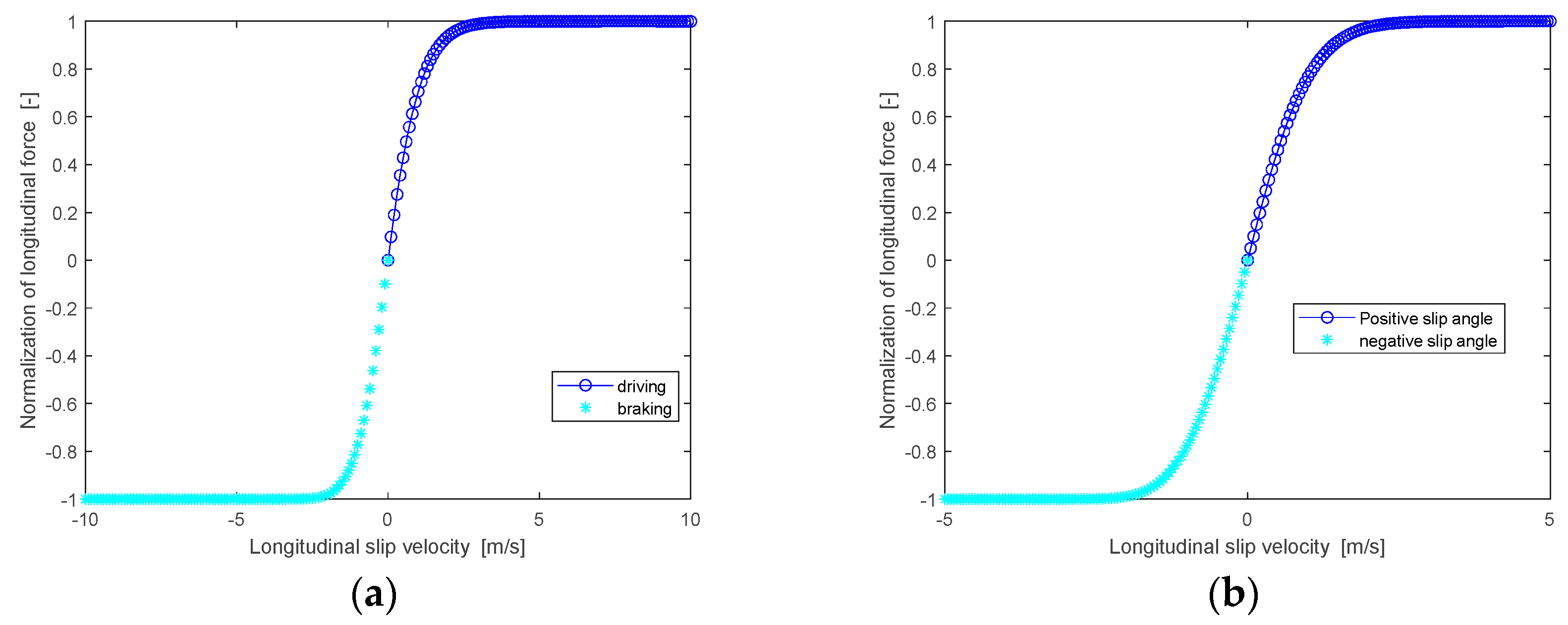
3.2. Normalization and Prediction Method for Tire Forces

Figure 10 shows the normalized longitudinal force and normalized lateral force of the four groups’ tires in Table 1 under three test loads, according to the method in Section 3.1. It can be seen that the normalized curves are not superimposed well due to the influence of contact pressure distribution.

However, when each group is considered separately and the load is distinguished, it can be found that the normalized curves of longitudinal force are superimposed very well under similar test condition, as shown in Figure 11.

Similarly, the lateral force of the two tires were normalized, as shown in Figure 12. It shows that the normalized lateral force curve is not as good as normalized longitudinal force curve, but it is still satisfactory.

The phenomenon that different tires could be yielding close to one normalized curve, which provides a good prediction inspiration. It means that the information of the reference tire can be applied without bringing too much error.

Referring to the dimensionless modeling method of UniTire tire model [56], the normalized curves of longitudinal force with respect to slip ratio and lateral force with respect to slip angle can be expressed as:

$$\{\begin{array}{l}\frac{F_x}{{\mu }_x{F}_z}=\overline{F_x}\left(\frac{K_x{S}_x}{{\mu }_x{F}_z}\right)=1-\exp \left(-\frac{K_x{S}_x}{{\mu }_x{F}_z}-E_{x1}\cdot {\left(\frac{K_x{S}_x}{{\mu }_x{F}_z}\right)}^2-\left(E_{x1}{}^2+E_{x2}\right)\cdot {\left(\frac{K_x{S}_x}{{\mu }_x{F}_z}\right)}^3\right)\\ \frac{F_y}{{\mu }_y{F}_z}=\overline{F_y}\left(\frac{K_y{S}_y}{{\mu }_y{F}_z}\right)=1-\exp \left(-\frac{K_y{S}_y}{{\mu }_y{F}_z}-E_{y1}\cdot {\left(\frac{K_y{S}_y}{{\mu }_y{F}_z}\right)}^2-\left(E_{y1}{}^2+E_{y2}\right)\cdot {\left(\frac{K_y{S}_y}{{\mu }_y{F}_z}\right)}^3\right)\end{array}$$

(13)

where $E_{x1}$ and $E_{x2}$ are the parameter of normalized longitudinal force, $E_{y1}$ and $E_{y2}$ are the parameter of normalized lateral force of the normalized model.

The dimensionless modeling using E index can well express the normalization curve, as shown in Figure 13. Importantly, the model can ensure that the boundary is equal to 1, which has a good effect on improving the prediction accuracy.

Combined with Equations (12) and (13), the longitudinal force and lateral force prediction model can be derived, as shown in Equation (14).

$$\{\begin{array}{l}{F}_x={\mu }_x{F}_z\overline{\cdot F_x}\left(\frac{K_x{S}_x}{{\mu }_x{F}_z}\right)\\ F_y={\mu }_y{F}_z\overline{\cdot F_y}\left(\frac{K_y{S}_y}{{\mu }_y{F}_z}\right)\end{array}$$

(14)

where the ${\overline{F}}_x$ and ${\overline{F}}_y$ is the normalized model of longitudinal force and lateral force from the reference tire; $F_z$ is the vertical load, ${\mu }_x$ and ${\mu }_y$ is the longitudinal and lateral dynamic friction, $K_x$ and $K_y$ is the longitudinal slip stiffness and cornering stiffness of the target tire; $F_x$ and $F_y$ is the longitudinal force and lateral force to be predicted.

According to Equation (14), in order to predict the tire longitudinal force or lateral force, it is necessary to obtain the longitudinal and lateral dynamic friction coefficient and slip stiffness. The prediction method of longitudinal and lateral dynamic friction coefficient has been given from Equation (1) to Equation (3), and the slip stiffness can be measured by linear zone test.

4. Tire Experiments and Validation

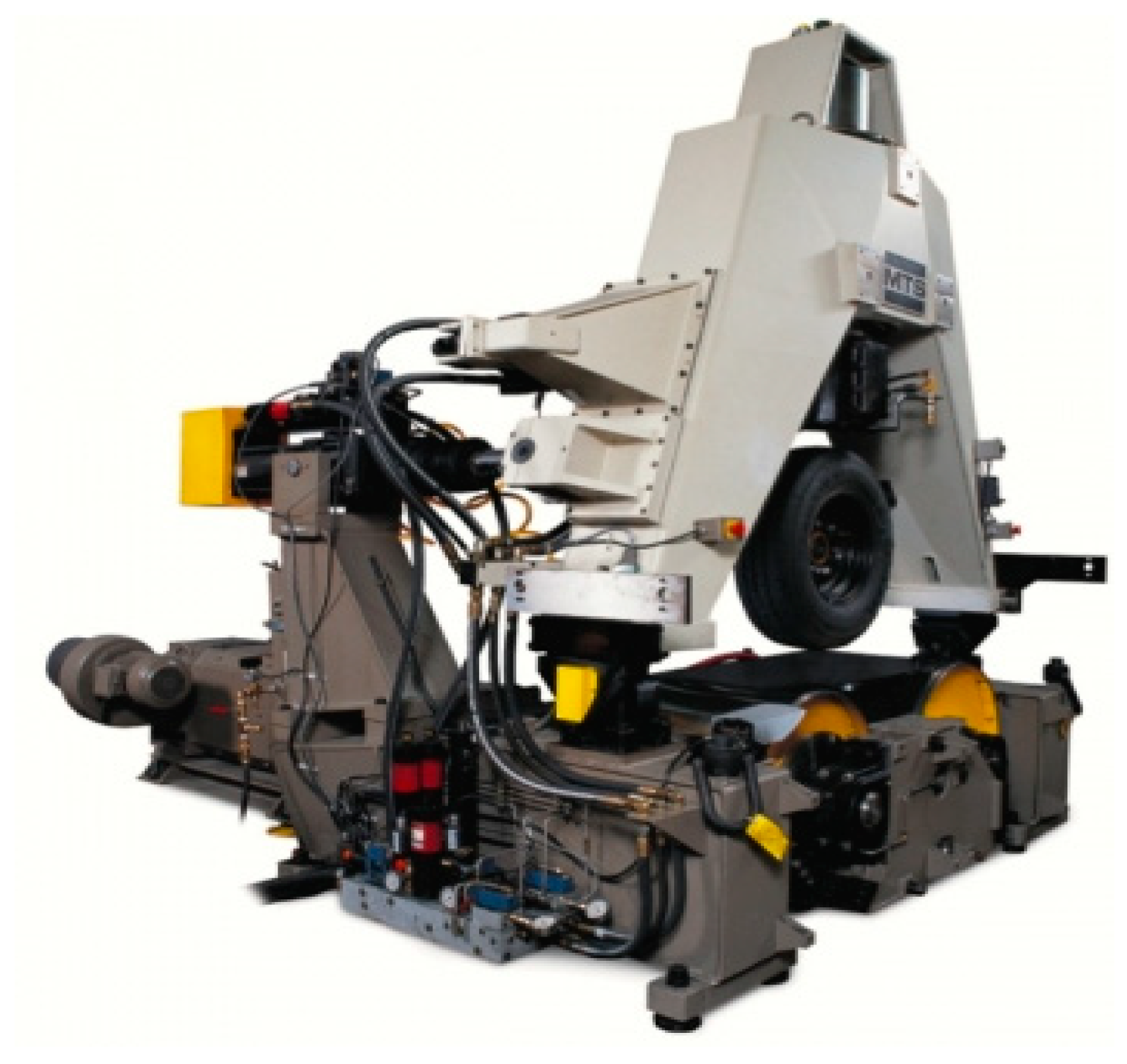
4.1. Experiments Design

The passenger tire of 215/55R18 was selected as the reference tire to predict the target tire of 215/60R17. The reference pressure ($P_{t0}$) of the target tire is 2.5 bar, and the reference load ($F_{z0}$) is 6958 N; the reference pressure ($P_{t0}$) of the reference tire is 2.5 bar, and the reference load ($F_{z0}$) is 6762 N. The test conditions for pure cornering and pure braking/driving are shown in

Table 4. The test conditions of pure cornering and pure braking/driving.

Item	Pt [%Pt0]	Vr [km/h]	γ [°]	Fz [%Fz0]	α [°]	κ [%]
Pure driving /braking	100	60	0	40, 80, 100	0	Sweep, rate = 10%/s −2→30 → −30 → 2
Pure cornering	100	60	0	40, 80, 100	Sweep, rate = 4°/s −2→15 → −15 → 2	0

.

The tire force tests were carried out on a Flat-trac machine (MTS System Corporation, Eden Prairie, MN, USA), as shown in Figure 1, and each tire has the same warm-up procedure to achieve thermal balance.

The test load is classified according to the percentage of the rated load, and the same rated load is divided into one category, so the load distribution under this condition is relatively similar.

4.2. Pure slip Stiffness Calculation

Measuring pure braking/driving and pure cornering test data with three loads, then the longitudinal slip stiffness and cornering stiffness are calculated, as shown in Figure 14.

Compared with the pure longitudinal slip test under large slip condition, the longitudinal force test data in the linear region is easier to obtain, and the tire has less tread wear and lower frictional heat.

4.3. Pure Longitudinal Force and Lateral Force Prediction Results

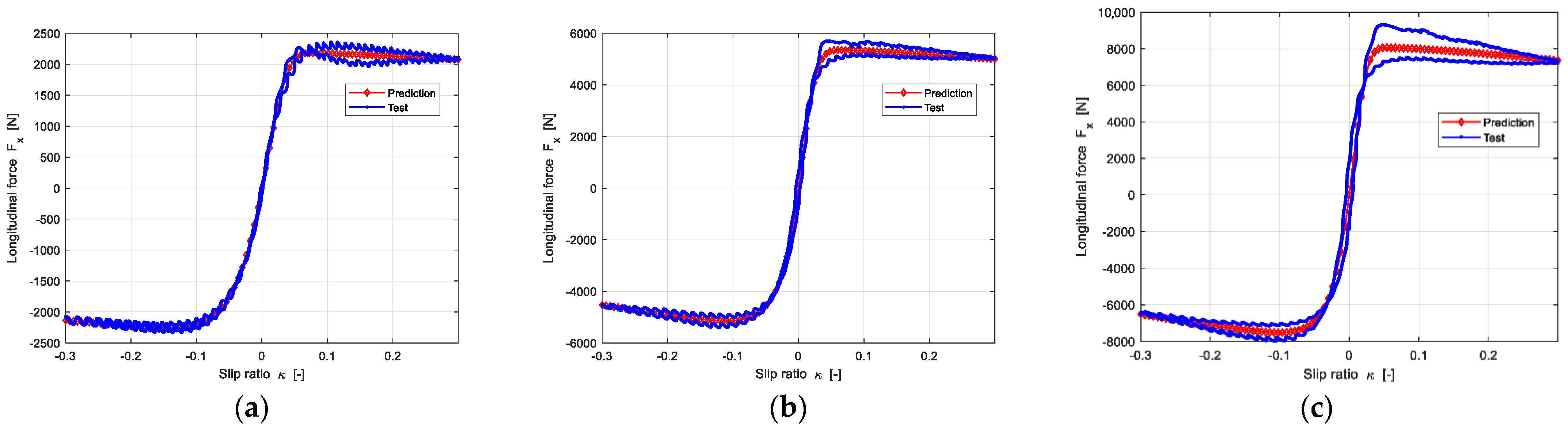
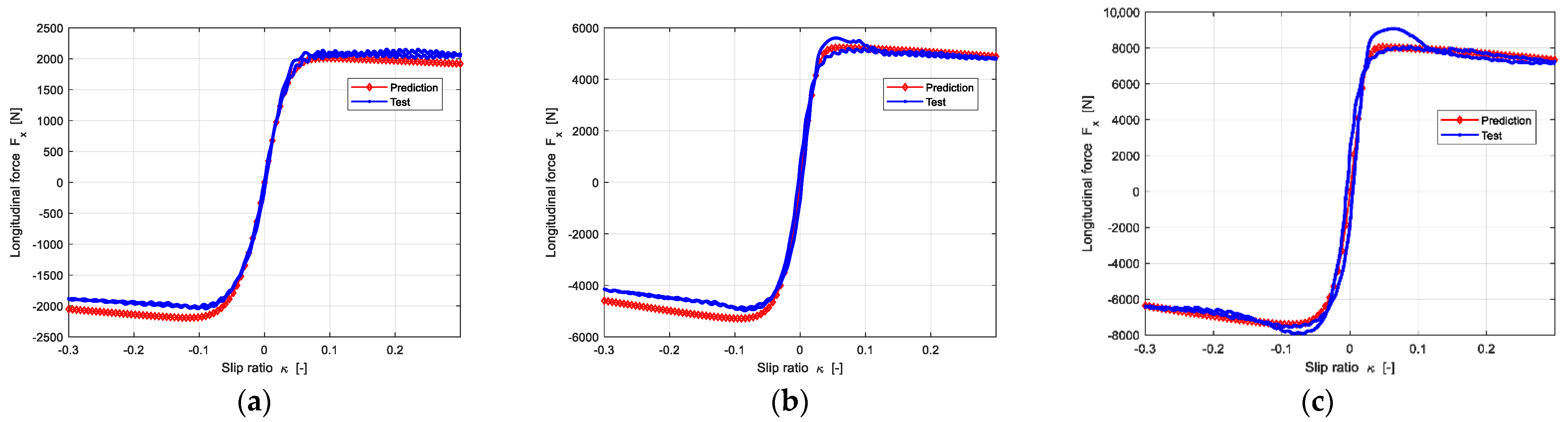
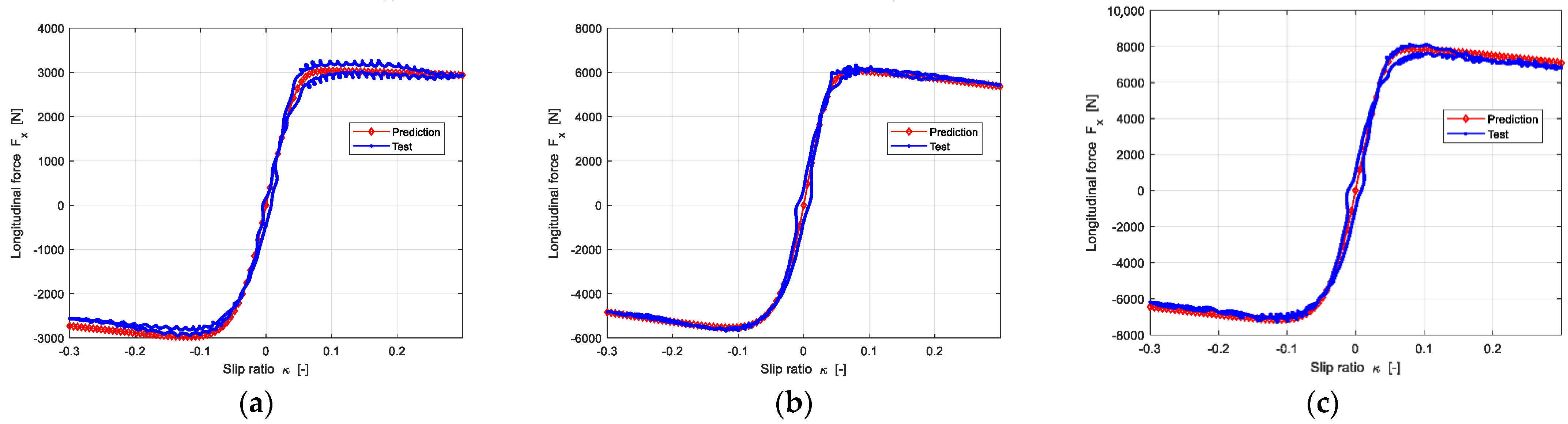
4.3.1. Pure Longitudinal Force

After measuring the longitudinal slip stiffness and acquiring the longitudinal friction through reference tire, then the longitudinal force can be predicted by Equation (13). The prediction results are shown in the Figure 15.

Figure 15 shows that the predicted longitudinal force is in good agreement with experimental data.

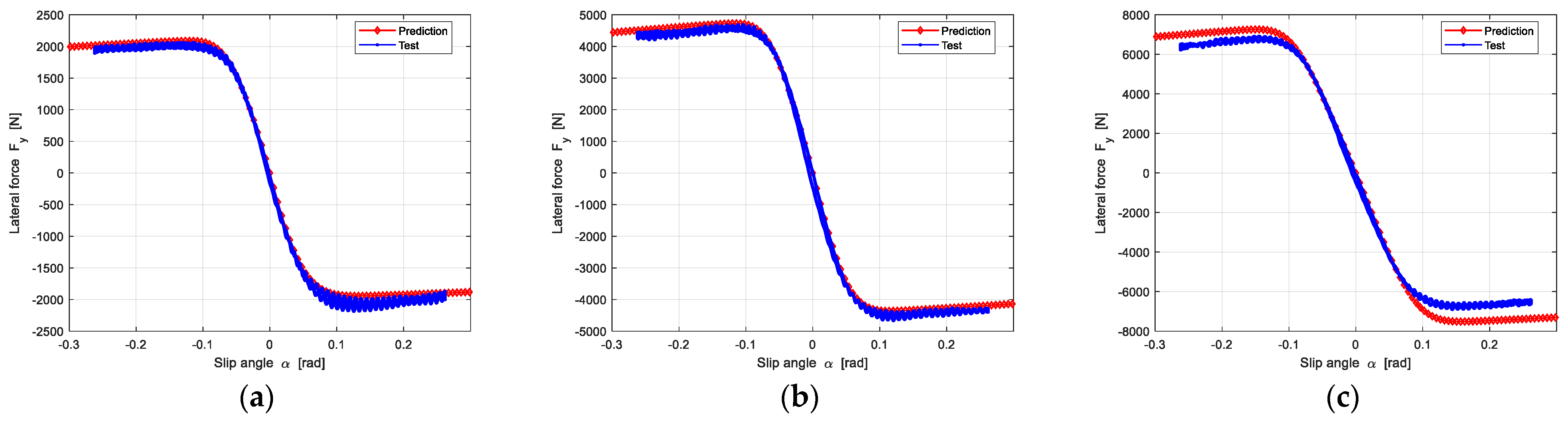
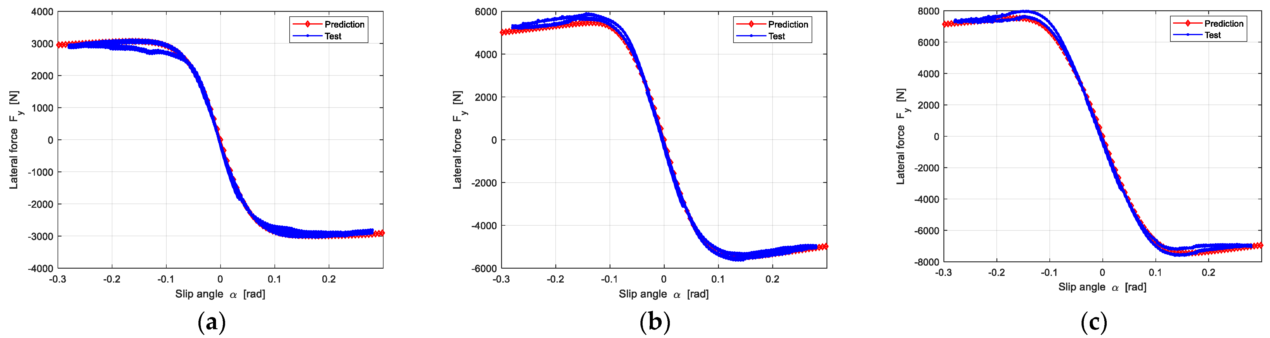
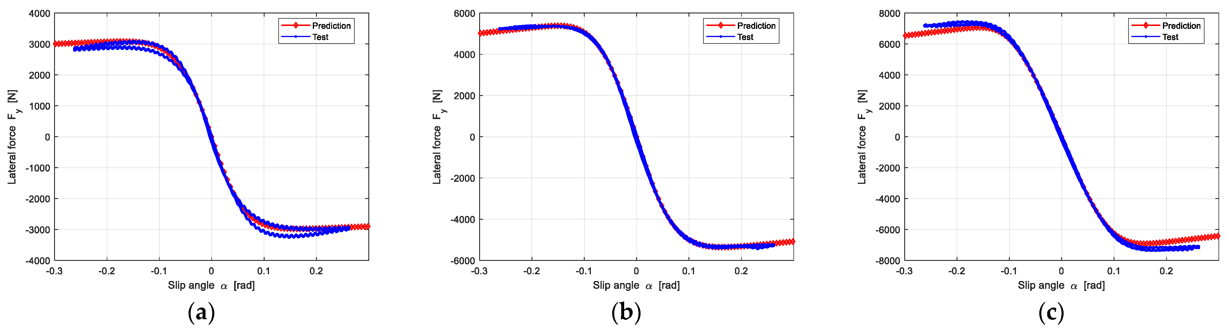
4.3.2. Pure Lateral Force

Similarity, the lateral force can be predicted when obtaining lateral slip stiffness and lateral friction. The prediction results are shown in Figure 16.

Figure 16 shows that the predicted lateral force is in good agreement with experimental data.

The prediction results of longitudinal force and lateral force of the other three groups are shown in Figure A1, Figure A2, Figure A3, Figure A4, Figure A5 and Figure A6, which are satisfactory as well.

The error index is defined as follow:

$$\{\begin{array}{l}{\epsilon }_{F_x}=\sqrt{\frac{{\displaystyle \sum _{i=1}^n{\left(F_{x_{Pred},i}-F_{x_{Meas},i}\right)}^2}}{{\displaystyle \sum _{i=1}^n{\left(F_{x_{Meas},i}\right)}^2}}}\\ {\epsilon }_{F_y}=\sqrt{\frac{{\displaystyle \sum _{i=1}^n{\left(F_{y_{Pred},i}-F_{y_{Meas},i}\right)}^2}}{{\displaystyle \sum _{i=1}^n{\left(F_{y_{Meas},i}\right)}^2}}}\end{array}$$

(15)

where $F_{xPred}$ and $F_{yPred}$ represent the predicted longitudinal force and lateral force from the model, $F_{xMeas}$ and $F_{yMeas}$ represent the measured longitudinal force and lateral force, and $n$ represents number of the test points.

The prediction errors of these sample tires in this paper are summarized in

Table 5. The prediction errors of tire forces.

Groups	${\mathit{F}}_{\mathit{x}} [\%]$	${\mathit{F}}_{\mathit{y}} [\%]$
1	8.63	2.79
2	8.10	5.98
3	10.15	3.18
4	4.68	3.24

below.

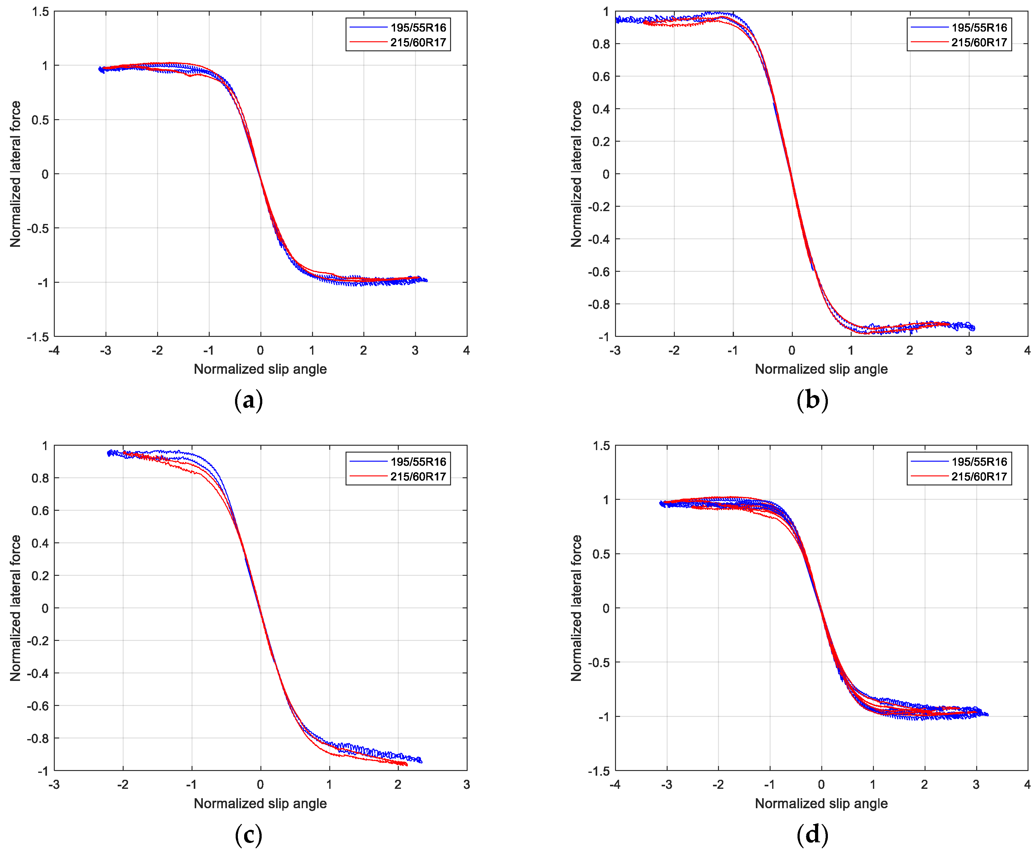
4.4. Analysis of Reference Tire Criteria

Through the prediction analysis of several samples, it is found that the longitudinal force and lateral force prediction method do not have very strict restrictions on the selection of reference tires. It is considered that the tires with similar specification to the target tire could be used as the reference tire. In order to improve the prediction accuracy of friction, it is recommended to classify the reference tires strictly, such as tire size, test conditions, and also tread pattern and compound.

In addition, the normalized characteristic curves from different machines are also analyzed and have the similar normalization phenomenon. However, considering the influence of frictional heat generation caused by the large slip test on the test data, it is necessary to identify the source of the reference tire, and it is recommended to make a detailed distinction according to test method and test conditions.

5. Discussion

In this paper, a separation and prediction method of tire dynamic friction characteristics is proposed. Based on the basic phenomenon of the normalization tire force curves of the reference tire and the target tire being highly overlapped, a prediction model and a prediction method of tire forces for the pure slip condition are proposed.

Compared with previous prediction models, the method in this paper has the following advantages:

Firstly, the normalization method in the literature need to measure a set of pure slip condition test data, as well as the slip stiffness and friction characteristics under the predicted vertical load. The method in this paper only needs to measure pure cornering force or pure longitudinal slip force, and slip stiffness, then another tire force can be effectively and efficiently predicted.

Secondly, the method in this paper realizes the separation of dynamic friction from the tire force, which lays the foundation for the high coincidence of normalized curves. However, the method in the literature does not realize friction separation, resulting in a poor normalization effect of the transition region due to friction differences, then it is impossible to use the reference tire information to achieve the purpose of prediction.

Thirdly, the dynamic friction can be predicted in this paper, however, the literature is based on experimental measurements. We proposed the concept of a reference tire, and using the reference tire information to predict the dynamic friction characteristics of the target tire. The experimental results show that the predicted dynamic friction is in good agreement with the experimental data.

Based on the above advantages, the prediction method in this paper has good predictive ability, which has important engineering value in reducing the tire modeling experiments and improving modeling efficiency.

However, this method also has certain limitations. On one hand, the proposed prediction method of dynamic friction needs to measure one of pure cornering force or pure longitudinal slip force. In the future, we would like to explore from a microscopic perspective to obtain the tire friction characteristics. On the other hand, we only study the prediction method of pure slip condition at present, and we will carry out the prediction research considering the inclination angle effect on tire force in the future.

6. Conclusions

The establishment of high-precision prediction models for tire longitudinal or lateral forces is of great significance for reducing tire force testing time and costs. In this paper, a new prediction method was presented based on slip stiffness and either pure cornering or driving/braking test data, which can efficiently and accurately predict the other pure slip mechanical properties. Some conclusions are summarized as follows:

Firstly, the method for separation of friction from test data under pure slip condition and the proportional assumption of longitudinal and lateral peak friction coefficient between target tire and reference tire are proposed. Moreover, the method and assumption are confirmed to be reasonable through experimental data, which provides a good basis for prediction of dynamic friction from a reference tire.

Secondly, a theoretical model considering the deformation of belt/carcass is established, which lays the foundation for the normalization model. According to the theoretical model, the contact pressure distribution characteristics will have an impact on the normalized curve, which is also naturally affected by the load. The normalization results under different loads verify the conclusion of the theoretical model analysis. However, under similar loads, the normalized curves of different tires are very close, which provides a good prediction foundation.

Thirdly, tire force tests were designed to verify the prediction ability of this model, and the results show that this prediction method can predict the tire longitudinal force or lateral force accurately. Compared with the cornering prediction, this prediction method is more meaningful for the prediction of longitudinal slip, especially when the testing machine is insufficient in measuring high loaded tires. Therefore, it has a good prospect of engineering application.

Fourthly, in the future, based on the research results of this paper, the slip stiffness of the designed tire can be obtained by the finite element method, and the relationship between the micro friction characteristics and the macro friction characteristics of the tire can be studied, which is of great significance for the virtual development of tires.

References

1. Kuiper, E.V.O.J.; Van Oosten, J.J.M. The PAC2002 advanced handling tire model. Veh. Syst. Dyn. 2007, 45 (Suppl. S1), 153–167. [Google Scholar] [CrossRef]
2. Pacejka, H.B. Tire and Vehicle Dynamics, 3rd ed.; Elsevier: Oxford, UK, 2012. [Google Scholar]
3. Pacejka, H.B.; Bakker, E. The magic formula tyre model. Veh. Syst. Dyn. 1993, 21 (Suppl. S1), 1–18. [Google Scholar] [CrossRef]
4. Pacejka, H.B.; Besselink, I.J.M. Magic formula tyre model with transient properties. Veh. Syst. Dyn. 1997, 27 (Suppl. S1), 234–249. [Google Scholar] [CrossRef]
5. Hirschberg, W.; Rill, G.; Weinfurter, H. Tire model tmeasy. Veh. Syst. Dyn. 2007, 45 (Suppl. S1), 101–119. [Google Scholar] [CrossRef]
6. Rill, G. TMeasy—A Handling Tire Model based on a three-dimensional slip approach. In Proceedings of the XXIII International Symposium on Dynamic of Vehicles on Roads and on Tracks (IAVSD 2013), Quingdao, China, 19–23 August 2013; pp. 19–23. [Google Scholar]
7. Rill, G. Road Vehicle Dynamics: Fundamentals and Modeling, 1st ed.; Taylor & Francis: Boca Raton, FL, USA, 2011. [Google Scholar]
8. Guo, K.; Lu, D.; Chen, S.K.; Lin, W.C.; Lu, X.P. The UniTire model: A nonlinear and non-steady-state tyre model for vehicle dynamics simulation. Veh. Syst. Dyn. 2005, 43 (Suppl. 1), 341–358. [Google Scholar] [CrossRef]
9. Guo, K.; Lu, D. UniTire: Unified tire model for vehicle dynamic simulation. Veh. Syst. Dyn. 2007, 45 (Suppl. S1), 79–99. [Google Scholar] [CrossRef]
10. Gim, G.; Choi, Y.; Kim, S. A semiphysical tyre model for vehicle dynamics analysis of handling and braking. Veh. Syst. Dyn. 2005, 43 (Suppl. S1), 267–280. [Google Scholar] [CrossRef]
11. Février, P.; Fandard, G. Thermal and mechanical tyre modelling for handling simulation. ATZ Worldw. 2008, 110, 26–31. [Google Scholar] [CrossRef]
12. Pearson, M.; Blanco-Hague, O.; Pawlowski, R. TameTire: Introduction to the model. Tire Sci. Technol. 2016, 44, 102–119. [Google Scholar] [CrossRef]
13. Jansen, S.T.; Verhoeff, L.; Cremers, R.; Schmeitz, A.J.; Besselink, I.J. MF-Swift simulation study using benchmark data. Veh. Syst. Dyn. 2005, 43 (Suppl. S1), 92–101. [Google Scholar] [CrossRef]
14. Schmeitz, A.J.C.; Besselink, I.J.M.; Jansen, S.T.H. Tno mf-swift. Veh. Syst. Dyn. 2007, 45 (Suppl. S1), 121–137. [Google Scholar] [CrossRef]
15. Gipser, M. FTire—the tire simulation model for all applications related to vehicle dynamics. Veh. Syst. Dyn. 2007, 45 (Suppl. S1), 139–151. [Google Scholar] [CrossRef]
16. Gipser, M. FTire and puzzling tyre physics: Teacher, not student. Veh. Syst. Dyn. 2016, 54, 448–462. [Google Scholar] [CrossRef]
17. Gallrein, A.; De Cuyper, J.; Dehandschutter, W.; Bäcker, M. Parameter identification for LMS CDTire. Veh. Syst. Dyn. 2005, 43 (Suppl. S1), 444–456. [Google Scholar] [CrossRef]
18. Gallrein, A.; Bäcker, M. CDTire: A tire model for comfort and durability applications. Veh. Syst. Dyn. 2007, 45 (Suppl. S1), 69–77. [Google Scholar] [CrossRef]
19. Oertel, C.; Fandre, A. Ride comfort simulations and steps towards life time calculations: RMOD-K tyre model and ADAMS. In Proceedings of the International ADAMS Users’ Conference, Berlin, Germany, 17–18 November 1999. [Google Scholar]
20. Oertel, C.; Fandre, A. Tire model RMOD-K 7 and misuse load cases. In SAE Technical Paper; SAE International: Warrendale, PA, USA, 2009. [Google Scholar] [CrossRef]
21. Flat-Trac Tire Test Systems [EB/OL]. Available online: http://www.mts.com/cs/groups/public/documents/library/dev_002227.pdf (accessed on 14 October 2014).
22. Xu, N.; Hashemi, E.; Tang, Z.; Khajepour, A. Data-Driven Tire Capacity Estimation with Experimental Verification. IEEE Trans. Intell. Transp. Syst. 2022, 1–13. [Google Scholar] [CrossRef]
23. Bhoopalam, A.K.; Sandu, C. Review of the state of the art in experimental studies and mathematical modeling of tire performance on ice. J. Terramech. 2014, 53, 19–35. [Google Scholar] [CrossRef]
24. Braghin, F.; Cheli, F.; Sabbioni, E. Environmental effects on Pacejka’s scaling factors. Veh. Syst. Dyn. 2006, 44, 547–568. [Google Scholar] [CrossRef]
25. Arosio, D.; Braghin, F.; Cheli, F.; Sabbioni, E. Identification of Pacejka’s scaling factors from full-scale experimental tests. Veh. Syst. Dyn. 2005, 43 (Suppl. S1), 457–474. [Google Scholar] [CrossRef]
26. Waluś, K.J. Experimental Determination of Vehicle Lateral Drift Characteristics under Laboratory Conditions. Appl. Mech. Mater. 2012, 232, 836–840. [Google Scholar] [CrossRef]
27. Persson, B.N.J. Rubber friction and tire dynamics. J. Phys. Condens. Matter 2010, 23, 015003. [Google Scholar] [CrossRef] [PubMed]
28. Lugaro, C.; Schmeitz, A.; Ogawa, T.; Murakami, T.; Huisman, S. Development of a parameter identification method for MF-Tyre/MF-Swift applied to parking and low speed manoeuvres. SAE Int. J. Passeng. Cars-Mech. Syst. 2016, 9, 892–903. [Google Scholar] [CrossRef]
29. Zhu, J.J.; Khajepour, A.; Spike, J.; Chen, S.K.; Moshchuk, N. An integrated vehicle velocity and tyre-road friction estimation based on a half-car model. Int. J. Veh. Auton. Syst. 2016, 13, 114–139. [Google Scholar] [CrossRef]
30. Liu, X.; Cao, Q.; Wang, H.; Chen, J.; Huang, X. Evaluation of vehicle braking performance on wet pavement surface using an integrated tire-vehicle modeling approach. Transp. Res. Rec. 2019, 2673, 295–307. [Google Scholar] [CrossRef]
31. Khaleghian, S.; Emami, A.; Taheri, S. A technical survey on tire-road friction estimation. Friction 2017, 5, 123–146. [Google Scholar] [CrossRef]
32. Acosta, M.; Kanarachos, S.; Blundell, M. Road Friction Virtual Sensing: A Review of Estimation Techniques with Emphasis on Low Excitation Approaches. Appl. Sci. 2017, 7, 1230. [Google Scholar] [CrossRef]
33. Wang, Y.; Hu, J.; Wang, F.A.; Dong, H.; Yan, Y.; Ren, Y.; Zhou, C.; Yin, G. Tire road friction coefficient estimation: Review and research perspectives. Chin. J. Mech. Eng. 2022, 35, 6. [Google Scholar] [CrossRef]
34. Kanafi, M.M.; Kuosmanen, A.; Pellinen, T.K.; Tuononen, A.J. Macro- and micro-texture evolution of road pavements and correlation with friction. Int. J. Pavement Eng. 2015, 16, 168–179. [Google Scholar] [CrossRef]
35. Du, Y.; Liu, C.; Song, Y.; Li, Y.; Shen, Y. Rapid Estimation of Road Friction for Anti-Skid Autonomous Driving. IEEE Trans. Intell. Transp. Syst. 2020, 21, 2461–2470. [Google Scholar] [CrossRef]
36. Leng, B.; Jin, D.; Xiong, L.; Yang, X.; Yu, Z. Estimation of tire-road peak adhesion coefficient for intelligent electric vehicles based on camera and tire dynamics information fusion. Mech. Syst. Signal Processing 2021, 150, 107275. [Google Scholar] [CrossRef]
37. Matsuzaki, R.; Kamai, K.; Seki, R. Intelligent tires for identifying coefficient of friction of tire/road contact surfaces using three-axis accelerometer. Smart Mater. Struct. 2014, 24, 025010. [Google Scholar] [CrossRef]
38. Paul, D.; Velenis, E.; Humbert, F.; Cao, D.; Dobo, T.; Hegarty, S. Tyre–road friction μ-estimation based on braking force distribution. Proc. Inst. Mech. Eng. Part D J. Automob. Eng. 2019, 233, 2030–2047. [Google Scholar] [CrossRef]
39. Müller, S.; Uchanski, M.; Hedrick, K. Estimation of the Maximum Tire-Road Friction Coefficient. ASME J. Dyn. Sys. Meas. Control 2003, 125, 607–617. [Google Scholar] [CrossRef]
40. Xia, X.; Xiong, L.; Sun, K.; Yu, Z.P. Estimation of maximum road friction coefficient based on Lyapunov method. Int. J. Automot. Technol. 2016, 17, 991–1002. [Google Scholar] [CrossRef]
41. Nishihara, O.; Masahiko, K. Estimation of Road Friction Coefficient Based on the Brush Model. ASME J. Dyn. Sys. Meas. Control 2011, 133, 041006. [Google Scholar] [CrossRef]
42. Liu, Y.-H.; Li, T.; Yang, Y.-Y.; Ji, X.-W.; Wu, J. Estimation of tire-road friction coefficient based on combined APF-IEKF and iteration algorithm. Mech. Syst. Signal Processing 2017, 88, 25–35. [Google Scholar] [CrossRef]
43. de Menezes Lourenço, M.A.; Eckert, J.J.; Silva, F.L.; Santiciolli, F.M.; Silva, L.C.A. Vehicle and twin-roller chassis dynamometer model considering slip tire interactions. Mech. Based Des. Struct. Mach. 2022, 1–18. [Google Scholar] [CrossRef]
44. Radt, H.S.; Glemming, D.A. Normalization of Tire Force and Moment Data. Tire Sci. Technol. TSTCA 1993, 21, 91–119. [Google Scholar] [CrossRef]
45. Radt, H.S., Jr.; Milliken, W.F., Jr. Non-dimensionalizing tyre data for vehicle simulation. In Proceedings of the Road Vehicle Handling, I Mech E Conference Publications 1983-5. Sponsored by Automobile Division of the Institution of Mechanical Engineers under Patronage of Federation Internationale des Societies d’Ingenieurs des Techniques de l’Automobile (FISITA) he (No. C133/83), Nuneaton, UK, 24–26 May 1983. [Google Scholar]
46. Kasprzak, E.M.; Lewis, K.E.; Milliken, D.L. Inflation pressure effects in the nondimensional tire model. SAE Trans. 2006, 115, 1781–1792. [Google Scholar]
47. Kasprzak, E.M.; Lewis, K.E. Tire asymmetries and pressure variations in the Radt/Milliken nondimensional tire model. In Proceedings of the SAE Automotive Dynamics, Stability and Controls Conference and Exhibition, Novi, MI, USA, 14–16 February 2006; pp. 1–1968. [Google Scholar]
48. Sharp, R.S. Testing and improving a tyre shear force computation algorithm. Veh. Syst. Dyn. 2004, 41, 223–247. [Google Scholar] [CrossRef]
49. Sharp, R.S.; Bettella, M. On the construction of a general numerical tyre shear force model from limited data. Proc. Inst. Mech. Eng. Part D J. Automob. Eng. 2003, 217, 165–172. [Google Scholar] [CrossRef]
50. Sharp, R.S.; Bettella, M. Shear Force and Moment Descriptions by Normalisation of Parameters and the “Magic Formula”. Veh. Syst. Dyn. 2003, 39, 27–56. [Google Scholar] [CrossRef]
51. Guo, K. Automotive Tire Dynamics; Science Press: Beijing, China, 2018; p. 1. (In Chinese) [Google Scholar]
52. Guo, K.H. A Unified Tire Model for Braking Driving and Steering Simulation. In Proceedings of the Fifth International Pacific Conference on Automotive Engineering, Beijing, China, 5–10 November 1989. [Google Scholar]
53. Fiala, E. Seitenkrafte am rollenden luftreifen (Lateral forces on rolling pneumatic tires). Z. VDI 1954, 96, 973–979. [Google Scholar]
54. Xu, N.; Guo, K.; Zhang, X.; Karimi, H.R. An Analytical Tire Model with Flexible Carcass for Combined Slips. Math. Probl. Eng. Theory Methods Appl. 2014, 2014, 397538. [Google Scholar] [CrossRef]
55. Sakai, H. Theoretical and Experimental Studies on the Dynamic Properties of Tyres, Part 2: Experimental Investigation of Rubber Friction and Deformation pf a Tyre. Ins. J. Veh. Des. 1981, 2, 182–226. [Google Scholar]
56. Guo, K.; Sui, J. A theoretical observation on empirical expression of tire shear forces. Veh. Syst. Dyn. 1996, 25, 263–274. [Google Scholar] [CrossRef]
Figure 1. Flat-trac machine.
Machines 10 00791 g001
Figure 2. The ratio of longitudinal and lateral peak friction at three different loads of the four groups: (a) The friction on the side of negative slip velocity; (b) The friction on the side of positive slip velocity.
Machines 10 00791 g002
Figure 3. The identification results of the longitudinal dynamic friction coefficient of the reference tire: (a) The Vertical load is 2783 N; (b) The Vertical load is 5566 N; (c) The Vertical load is 6958 N.
Machines 10 00791 g003
Figure 4. The identification results of the lateral dynamic friction coefficient of the reference tire: (a) The Vertical load is 2783 N; (b) The Vertical load is 5566 N; (c) The Vertical load is 6958 N.
Machines 10 00791 g004
Figure 5. The identification results of the longitudinal dynamic friction coefficient of the target tire: (a) The Vertical load is 2705 N; (b) The Vertical load is 5410 N; (c) The Vertical load is 6762 N.
Machines 10 00791 g005
Figure 6. The identification results of the lateral dynamic friction coefficient of the target tire: (a) The Vertical load is 2705 N; (b) The Vertical load is 5410 N; (c) The Vertical load is 6762 N.
Machines 10 00791 g006
Figure 7. Longitudinal dynamic friction comparisons between test data and prediction results of the target tire: (a) The Vertical load is 2705 N; (b) The Vertical load is 5410 N; (c) The Vertical load is 6762 N.
Machines 10 00791 g007
Figure 8. Lateral dynamic friction comparisons between test data and prediction results of the target tire: (a) The Vertical load is 2705 N; (b) The Vertical load is 5410 N; (c) The Vertical load is 6762 N.
Machines 10 00791 g008
Figure 9. Deformations of tread and belt/carcass in contact patch under combined slip condition.
Machines 10 00791 g009
Figure 10. The normalized longitudinal force and normalized lateral force of the four groups tires under three test loads: (a) Normalized longitudinal force; (b) Normalized lateral force.
Machines 10 00791 g010
Figure 11. Normalized curves of longitudinal force between two different tires: (a) Normalized longitudinal force under small load; (b) Normalized longitudinal force under middle load; (c) Normalized longitudinal force under high load; (d) Normalized longitudinal force with three loads.
Machines 10 00791 g011
Figure 12. Normalized curves of lateral force between two different tires: (a) Normalized lateral force under small load; (b) Normalized lateral force under middle load; (c) Normalized lateral force under high load; (d) Normalized lateral force with three loads.
Machines 10 00791 g012
Figure 13. Normalized curves of longitudinal force and lateral force: (a) Normalized longitudinal force for zero slip angle.; (b) Normalized lateral force for zero inclination angle.
Machines 10 00791 g013
Figure 14. Test results of longitudinal slip stiffness and cornering stiffness: (a) Longitudinal slip stiffness at three loads; (b) Cornering stiffness at three loads.
Machines 10 00791 g014
Figure 15. The prediction results of longitudinal force under three different loads: (a) The Vertical load is 2705 N; (b) The Vertical load is 5410 N; (c) The Vertical load is 6762 N.
Machines 10 00791 g015
Figure 16. The prediction results of lateral force under three different loads: (a) The Vertical load is 2705 N; (b) The Vertical load is 5410 N; (c) The Vertical load is 6762 N.
Machines 10 00791 g016