A Novel Sliding Mode Momentum Observer for Collaborative Robot Collision Detection

Abstract

Safety during physical human–robot interaction is the most basic requirement for robots. Collision detection without additional sensors is an economically feasible way to ensure it. In contrast, current collision detection approaches have an unavoidable trade-off between sensitivity to collisions, signal smoothness, and immunity to measurement noise. In this paper, we present a novel sliding mode momentum observer (NSOMO) for detecting collisions between robots and humans, including dynamic and quasistatic collisions. The collision detection method starts with a dynamic model of the robot and derives a generalized momentum-based state equation. Then a new reaching law is devised, based on which NSOMO is constructed by fusing momentum, achieving higher bandwidth and noise immunity of observation. Finally, a time-varying dynamic threshold (TVDT) model is designed to distinguish between collision signals and the estimated lumped disturbance. Its coefficients are obtained through offline data recognition. The TVDT with NSOMO enables fast and reliable collision detection and allows collision position assessment. Simulation experiments and hardware tests of the 7-DOF collaborative robot are implemented to illustrate this proposed method’s effectiveness.

1. Introduction

In recent years, robot manipulators have been increasingly used in industrial manufacturing and aerospace applications. In these complex applied environments, humans can work with manipulators to accomplish tasks [1]. During working, the collision between robots and human is inevitable. It may be a dynamic collision or static extrusion. Potential harm to humans from robot manipulators is in summary in [2]. On the other hand, many researchers have developed motion planning algorithms to avoid collisions in advance [3,4]. Therefore, the safety technology of physical human–robot interaction (pHRI) has become a key technology in robotics. It is crucial to detect the location and size of collision timely and accurately, making it a promising practical application to promote safe pHRI.

Thanks to the development of mechatronics technology, robot manipulators currently used in industry are equipped with collision detection for safe pHRI [5]. They are divided into requiring external sensors and using only propriety sensors (encoders, actuating motors). External sensors, e.g., electronic skin [6], six-dimensional force/torque sensors, and inertial devices, assist in judgment [7]. Its precision depends primarily on external sensors’ measurement accuracy. However, it dramatically increases the structural complexity and manufacturing cost of robot systems. Techniques using only proprioceptive sensors are then explored, actuator current changes at joints is a basic way to determine whether a collision occurs [8]. However, the underlying current signal is usually full of noise and subject to high external interference, so it is not entirely accurate. Later influenced by the idea of state observers in classical control theory, collision state observer is constructed by a system’s control output and the available system’s output state [9]. Various disturbance observers are derivative of state observers, primarily for observing disturbances (collisions can also be seen as an external disturbance) [10]. It is widely used in control, and a detailed review of disturbance observers is given in [11].

Based on the analysis above, it is evident that constructing a suitable state observer is the key to utilizing only propriety sensor techniques. In constructing state observer techniques, there are model-based and model-free approaches [12]. As its name implies, model-free methods do not require model-specific information. A large amount of usable data drives them to achieve state observations [13]. This data-driven idea has extensive applications in industrial monitoring [14,15] and fault diagnosis [16,17]. Artificial intelligence techniques as a typical data-driven technology are developing rapidly. Detection algorithms via neural networks (NN) [18], support vector machines (SVM) [19], or fuzzy systems [20] have also become an important development direction for model-free methods. Such intelligent methods are cost-effective compared to external sensors. Nevertheless, the low model information means extensive experimental data must be collected [21]. In addition, the trained model’s generality is worth verifying, and it will impose a computational burden on the controller, so it may not be suitable for other robot systems.

However, model-based methods can avoid the drawbacks of model-free methods. In model-based approaches, in order to build appropriate state observers for collision detection, early studies have tried using energy observer [22], joint velocity observer [23], momentum feedback disturbance observer [24], and even directly using robot manipulator model parameters to calculate external collision torque [25]. Although such ways require only model information, they are also susceptible to model errors. Moreover, they need to calculate joint acceleration signals, which are often noisy due to sensor data differentiation. Until a generalized momentum observer (GM) is proposed in [26], it allows easy implementation and promotion without solving acceleration signals and inertia matrix inversion. The GM is widespread in fields such as robot collision detection or fault diagnosis [27]. The GM is essentially a first-order filter of external torque [28]. Although the noise in the external torque signal can be filtered out, it also tends to ignore the fast and abrupt external torque signal. In order to improve the rapidity of GM, an additional high-pass filter and proportional differentiation loop are added to optimize the detection rate further [29]. Similar linear filtering improvement methods available in [30], which are insufficient to cope with nonlinear torque variations. Another critical factor affecting detection sensitivity is the collision threshold. The conventional collision threshold is a fixed value, which will reduce accuracy if it is too high and cause collision misclassification if it is too low [31]. Thus, the time-varying collision threshold is later explored to distinguish collision signals from noisy signals like an internal disturbance in real time [32]. The usual practice is to build a time-varying threshold model by modeling each joint with internal torque. As a result, finding an accurate and easy-to-use threshold model has become a technical challenge.

Although the GM method still has unsatisfactory aspects, there is no doubt that momentum has become the best state for collision detection. Consequently, integrating GM with other techniques has become a new trend. Model parameter identification and GM can be fused to obtain system model information [33] or raise detection speed using adaptive model techniques [34]. Another scholar constructs a collision network by combining GM and deep neural network (DNN) to perform collision detection [35]. Such methods are certainly novel, but they still require a lot of model training and computation. In order to alter the drawbacks of GM with fixed gain, it is natural to consider integrating momentum into the Kalman filter. The GM is extended to the Kalman filter technique in [36] to estimate momentum and external collision torque. It has high noise immunity, but the accuracy of its estimation depends heavily on model accuracy. Second-order and higher-order observers have the merits of fast-tracking, and their combination with GM is a new attempt. The extended state observer (ESO) is designed to be fused with GM to improve the bandwidth of collision detection [12]. A higher-order finite-time observer is merged with the GM to achieve fast time-varying external force estimation [37]. However, it brings a corresponding complexity to algorithms and the problem of balancing fast response and noise suppression. The super-twisting algorithm (ST), a typical high-order sliding mode technique, is first coupled with GM to form a sliding mode momentum observer (SOMO) to estimate external torque and joint angular acceleration simultaneously [38]. However, the chattering phenomenon still exists in practice, and increasing order also brings certain hysteresis. Sliding mode techniques originate from variable structure control not only limited to ST algorithms. The nature of the sliding mode technique lies in reaching law design. Moral reaching law can enhance the system’s comprehensive performance [39].

Given discussion and analysis in previous work mentioned above, along with being inspired by GM and SOMO ideas, we further explored the potential of sliding mode and GM technique. Therefore, this paper designs a novel sliding mode momentum observer (NSOMO) coupled with the time-varying dynamic threshold (TVDT) for collision detection without external sensors to improve detection sensitivity and accuracy. Figure 1 illustrates the benefits of this proposed collision detection solution. The TVDT in Figure 1 also refers to the time-varying dynamic threshold. In addition, the main contributions of this paper’s work are:

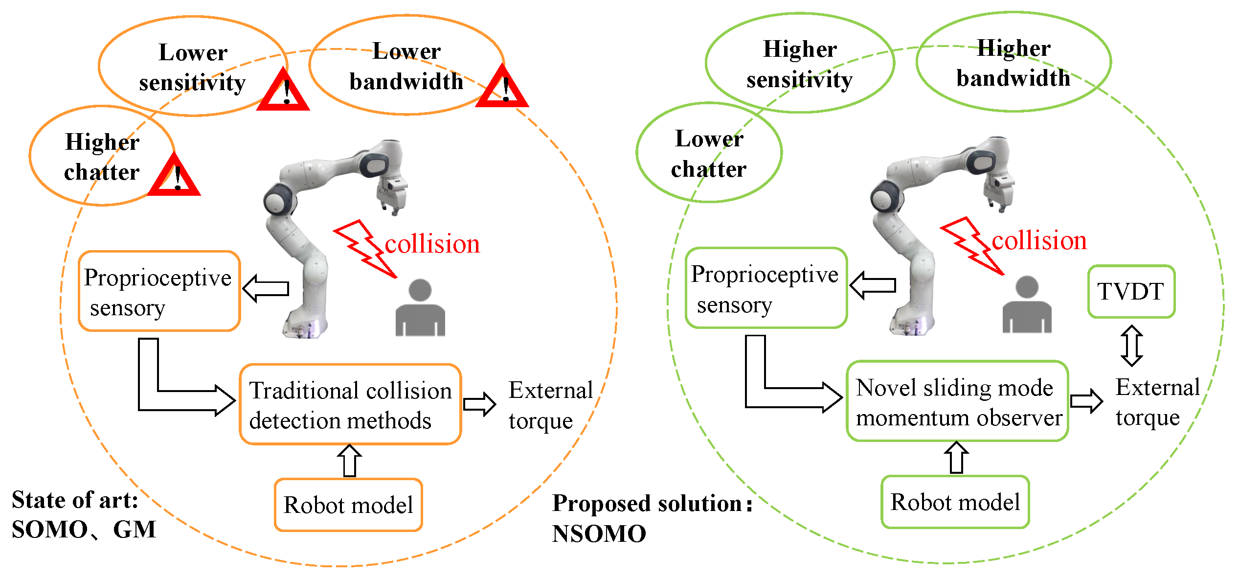
• In order to achieve the required bandwidth and noise immunity for collision detection, a new reaching law (NRL) is designed. The NSOMO is also proposed, exhibiting a slight external torque detection delay, a high external torque estimation accuracy and a small jitter phenomenon. Furthermore, NSOMO can be applied to any robot manipulator, providing a new idea for collision detection technology.
• To further increase detection sensitivity, a TVDT model was constructed by parameter identification of the joint disturbance torque model using offline data. This model can distinguish collision signals from estimated lumped disturbance. It also offers a way to identify collision location based on collision signal.
• Complete stability analysis and reaching time calculation were provided for NRL. For NSOMO, a comprehensive stability proof and a stable region were analyzed. It gives theoretical support for generalizing this approach to other robot systems.

For actual validation, we used an excellent collaborative robotics research platform—Franka emika [40]. The offline data were first processed using the least-squares method to obtain DVDT model parameters. Then a practical model validation test was done to ensure the effectiveness. External torque detection test and human–machine interaction crash experiment were then executed. Note that quasistatic squeezing is also considered in the external torque detection test, while GM, SOMO, and NSOMO are compared with the platform’s torque sensor. The results indicate that this collision detection solution can respond faster to collisions, ensuring a safe pHRI.

The rest of this paper is organized as follows. In Section 2, the dynamic model and preparation of robot are described. Section 3 provides a design process for GM, SOMO and NSOMO. The theoretical analysis is then given. Section 4 presents an overall collision detection strategy, including the TVDT model and collision position assessment and response. In Section 5, a simulation test to verify the proposed collision detection method. Section 6 conducts a practical experimental validation to illustrate a collision detection solution’s general performance. Finally, Section 7 is the conclusion of this paper.

2. Preliminaries

2.1. Model of Robot Dynamics

To build a novel observer-based collision detection algorithm, we could take the n-link robot as a rigid body at first, then construct its dynamic model as:

$$M\left(q\right)\ddot{q}+C(q,\dot{q})\dot{q}+G\left(q\right)=\tau +{\tau }_{ext}$$

(1)

where $q,\dot{q},\ddot{q}\in R^n$ represent the joint angle, angular velocity, and angular acceleration of the manipulator, respectively; $M\left(q\right)\in R^{n\times n}$ is the symmetric positive definite inertia matrix; $C(q,\dot{q})\in R^{n\times n}$ is the Coriolis matrix, which signifies the effect of Coriolis force and centrifugal force on joints. $G(q,\dot{q})\in R^{n\times 1}$ indicates the gravity matrix; $\tau \in R^{n\times 1}$ is the actuator output torque vector on each joint of the manipulator. ${\tau }_{ext}\in R^{n\times 1}$ denotes the actual external disturbance torque vector generated by the collision between the manipulator and physical environment.

The actuator also has its dynamic model, mixed with other frictional torque disturbances, making it more complex. For simplicity, we consider only the rigid-body dynamic model in Equation (3). Meanwhile, to make the model more accurate, we must compensate for other unmodelled disturbance torque models.

These disturbance torque models can be analyzed based on the frequency and categorized as joint speed related or others. The joint damping torque, friction torque, and dynamic model error torque, whose model equations are illustrated in Equation (2), have signal frequencies determined by the change in joint velocity [41]. The frequency of sensor measurement noise and other environment noise disturbances will be far higher than the joint speed change rate.

$$\begin{array}{cc}\hfill {\tau }_v& =B\dot{q}\hfill \\ \hfill {\tau }_f& =T_{k}sign\left(\dot{q}\right)\hfill \\ \hfill {\tau }_m& =\Delta M\left(q\right)\frac{d}{dt}\dot{q}+\frac{1}{2}{\dot{q}}^T\frac{\partial \Delta M}{\partial q}\dot{q}-\Delta g\left(q\right)\hfill \end{array}$$

(2)

where ${\tau }_v\in R^{n\times 1},{\tau }_f\in R^{n\times 1},{\tau }_m\in R^{n\times 1}$ are the joint damping torque, joint friction torque, and dynamic model error torque, respectively. $B, T_k$ are the damping and dynamic friction torque coefficients, respectively. $\dot{q}$ indicates the joint angular velocity. $\Delta M\left(q\right)$ is the mass error of model. $\Delta g\left(q\right)$ represents the effect of mass error on gravity. $sign(·)$ stands for symbolic functions. $\frac{d}{dt}, \frac{\partial }{\partial q}$ denote the derivative to time and partial differentiation to joint velocity, respectively.

Therefore, the Equation (3) can be reformulated as:

$$M_0\left(q\right)\ddot{q}+C_0(q,\dot{q})\dot{q}+G_0\left(q\right)+\rho =\tau +{\tau }_{ext}$$

(3)

with

$$\rho =\Delta M\left(q\right)\frac{d}{dt}\dot{q}+\frac{1}{2}{\dot{q}}^T\frac{\partial \Delta M}{\partial q}\dot{q}+B\dot{q}-\Delta g\left(q\right)+T_{k}sign\left(\dot{q}\right)+{\epsilon }_n+{\epsilon }_b$$

(4)

where $M_0\in R^{n\times n},C_0\in R^{n\times n},G_0\in R^{n\times 1}$ are modeling known terms, $\rho \in R^{n\times 1}$ represents the total internal disturbance torque. ${\epsilon }_n\in R^{n\times 1}$ denotes the sensor measurement noise, and ${\epsilon }_b\in R^{n\times 1}$ means other noise. Thus the more accurately the total internal disturbance torque $\rho$ is calculated, the more accurately the external collision torque ${\tau }_{ext}$ will be estimated.

In addition, the robot model in Equation (3) has the following properties and assumptions, that will be employed in later analysis:

Property 1.

The matrix $M\left(q\right)-2C(q,\dot{q})$ is skew-symmetric and thus yields:

$$\dot{M}\left(q\right)=C(q,\dot{q})+C^T$$

(5)

where $C^T$ is the transpose of C.

Assumption 1.

${\tau }_{ext}$ is bounded, and $\left|{\tau }_{ext}\right|<\Delta$. where $\Delta >0$ is the boundary value.

2.2. Basic Sliding Mode Theory Knowledge

Completed research on sliding mode theory is available in [42]. This section briefly introduces its basic theory and significant benefits and drawbacks. To better understand sliding mode control techniques, we establish the following second-order nonlinear system:

$$\ddot{x}=f(x,\dot{x})+b(x,\dot{x})·u$$

(6)

where both f and b are nonlinear functions concerning $x, \dot{x}$, the b is invertible. Let $x_d$ be the standard trajectory while $e=x-x_d$ be the tracking error. Then the first step in sliding mode control is to design an appropriate sliding surface S. The universal design is:

$$S=\lambda e+\dot{e}$$

(7)

The next stage is designing the control law to make phase trajectories beyond the slide surface reach the slide surface in finite time, that is, the reaching phase. After reaching the slide surface, the system slides along the slide surface and gradually stabilizes to the equilibrium point, namely the slide phase. Figure 2 describes the system motion states for these two phases. In the reaching phase, the error vector $(e, \dot{e})$ is absorbed into the slide surface $S=0$. In the slide phase, the error vector “slides” on the slide surface until it converges to the equilibrium point $(0,0)$, the convergence rate is directly related to the value of $\lambda$.

To achieve the above demands, the control law should be designed to satisfy the following conditions, also known as reaching conditions:

$$S·\dot{S}<0,\forall t$$

(8)

In order to satisfy condition in Equation (8), in the conventional sliding mode method, S is designed as:

$$\dot{S}=-k·sign\left(S\right),\forall t,k>0$$

(9)

The arrival time $t_r$ shown in Equation (21) can be obtained by integrating Equation (8) with respect to time. This corresponds to the time required for the error vector $(e, \dot{e})$ to reach S.

$$t_r=\frac{\left|S\right(0\left)\right|}{k}$$

(10)

Equation (9) design, which contains a sign function, leads to chattering during the sliding process. Moreover, the extent of chattering is directly determined by k. Thus, a dilemma arises: increasing k yields faster convergence and tracking performance, while directly enlarging the level of chatter.

Equation (9), also named the reaching law approach, was proposed by Professor Weibing Gao based on the sliding mode control process [43]. The main idea is to develop a reaching equation for sliding mode surfaces so that the overall dynamic response of the system can be improved by adjusting the reaching law. For example, Equation (9) can also be modified to the following exponential reaching law [43]:

$$\dot{S}=-\epsilon ·sign\left(S\right)-ks,\forall t,k>0,\epsilon >0$$

(11)

By adjusting the parameters $\mathcal{E}$ and k, the convergence speed of the system can be accelerated while attenuating the chattering phenomenon. Therefore, additional methods of reaching laws have been proposed, such as power exponential reaching laws [43], exponential reaching laws [44], novel adaptive reaching laws [39].

3. Novel Sliding Mode Momentum Observer Design

An generalized momentum-based observer to detect external torques has been proposed in [45]. The approach is widely applied because it avoids the inverse operation of $M\left(q\right)$ and acceleration solving. A primary second-order sliding mode momentum observer is also presented in [38], and conclusions are given. This section first analyzes the principles of these two observers. Meanwhile, to consider these two observers’ advantages and improve overall observation performance, we propose a novel sliding mode momentum observer utilizing the reaching law approach. Further analysis of the properties was conducted.

3.1. Observer Design

General momentum p and its derivative in time are given by

$$\left\{\begin{array}{c}\hfill p=M\left(q\right)\dot{q}\hfill \\ \hfill \dot{p}=\dot{M}\left(q\right)\dot{q}+M\left(q\right)\ddot{q}\hfill \end{array}\right.$$

(12)

Then incorporating Equation (3) and Property 1, the first-order momentum p dynamic equation can be derived as

$$\dot{p}=\tau +C^T(q,\dot{q})\dot{q}-G\left(q\right)+{\tau }_{ext}-\rho$$

(13)

Then the generalized momentum method is organized as

$$\begin{array}{cc}\hfill & \hfill \dot{\widehat{p}}=\tau -\rho +C^T(q,\dot{q})\dot{q}-G\left(\dot{q}\right)+K(p-\widehat{p})\hfill \\ \hfill & \hfill r=K(p-\widehat{p})\hfill \end{array}$$

(14)

where $r\in R^{n\times 1}$ is the defined residual variable, $\widehat{p}\in R^{n\times 1}$ is the momentum estimate, and $K\in R^{n\times 1}>0$ is the vector gain. The main idea of this structure is to estimate external collision torque based on the proportional multiplier of momentum deviation. It is essentially a linear first-order low-pass filter, which can improve estimation convergence speed and ensure stability by increasing the gain K. However, a high gain will reduce the estimated noise immunity while failing to cope with the nonlinear variation. A good compromise between speed and accuracy is hard to achieve.

Subsequently, second-order momentum observer approaches such as extended state observer [12] and sliding mode momentum observer are researched. The extended state observer method for estimating external collision torque is prone to a “peak phenomenon” [32]. The basic structure of the sliding mode momentum observer [38] is

$$\begin{array}{cc}\hfill & \hfill \dot{\widehat{p}}=\tau -\rho +C^T(q,\dot{q})\dot{q}-G\left(q\right)+T{\left|\tilde{p}\right|}^{\frac{1}{2}}sign\left(\tilde{p}\right)+\sigma \hfill \\ \hfill & \hfill \dot{\sigma }=Qsign\left(\tilde{p}\right)\hfill \end{array}$$

(15)

where $\tilde{p}=p-\widehat{p}$ is the momentum deviation, $Q, T\in R^{n\times n}$ are positive definite symmetric matrix, the algorithm can realize the estimation of ${\tau }_{ext}$, namely $\sigma \approx {\tau }_{ext}$. The second-order sliding mode technique ensures that the observer converges in finite time. However, raising order also introduces a certain lag that affects rapidity. The symbolic function is bound to bring specific chattering problems.

We find it challenging to estimate external torque quickly and accurately. Adopting the reaching law based on the generalized momentum observer is triable towards the purpose. Design a new convergence law that improves fastness and can apply to nonlinear cases. The power rate reaching law (PRRL) is a well-used method to achieve smooth entry into sliding modes and eliminate chattering. Nevertheless, the convergence speed is languid when far from the sliding mode surface [43]. In this way, inspired by the work of [46], the double power rate reaching law (DPRRL) provides better global fast convergence performance. Designing a DPRRL initially as

$$\dot{S}=-k_1·{\left|S\right|}^{1-\beta }sgn\left(S\right)-k_2{\left|S\right|}^{1+\beta }sgn\left(S\right)$$

(16)

where $k_1>0,k_2>0$ are the reaching law coefficients, $0<\beta <1$, sgn() is the Symbolic function. When system states are closer to sliding mode surfaces, the rate of convergence is mainly determined by $-k_1·{\left|S\right|}^{1-\beta }sgn\left(S\right)$; when they are farther away, it is mainly determined by $-k_2·{\left|S\right|}^{1+\beta }sgn\left(S\right)$, which converges faster than exponential convergence. Compared to [46], the DPRRL in this paper also has a fast convergence rate with second-order sliding mode properties [47]. Therefore, it can guarantee the fast chatter-free convergence to the sliding mode surface. In addition, the DPRRL in Equation (16) has the advantage of fewer parameters with simple convergence time calculation.

This way, the convergence speed can be adjusted by simply tuning $\beta$. If increasing $\beta$ to ensure reaching speed when far from the slide surface, the value of $1-\beta$ will be lower at the cost of signal chattering when approaching slide mode surfaces. For smaller values of $\beta$, a chatter will be reduced, yet convergence will be slower when far from slide surface. Additionally, the value of $1-\beta$ increases, affecting system robustness [44]. Hence the compromise between rapidity and smoothness of DPRRL is crucial to regulate.

The chattering is treated as a result of excessive control near slide surfaces [48]. If it is possible to adaptively adjust the gain of reaching law to realize variable speed reaching law, it can prevent excessively action and eliminate chattering production. With this idea, a scaling function is devised such that the gain varies with the magnitude of the error. Incorporating the designed DPRRL in Equation (16), a new reaching law (NRL) can be obtained in the form of

$$\dot{S}=-\frac{k}{\mu +(1-\mu )e^{-\alpha \left|S\right|}}·\left[{\left|S\right|}^{1-\beta }sgn\left(S\right)+k_2{\left|S\right|}^{1+\beta }sgn\left(S\right)\right]$$

(17)

where $0<\mu <1,\alpha >0,k>0$. Here, the overall gain $K_i$ of the controller is adaptively changing according to the value of the switching function $\left|S\right|$. The variation rule is: when $S\to \infty$, the function $e^{-\alpha \left|S\right|}\to 0$, and the overall gain $K_i=k/\mu$; when $S\to 0$, the function $e^{-\alpha \left|S\right|}\to 1$, and the overall gain $K_i=k$. Thus overall gain varies within the interval $[k,k/\mu ]$. The lower the value of $\mu$, the wider the range of interval variation. It ensures fast convergence when away from the slide surface and reduces the chance of excessive control near the slide surface, thus weakening the system chatter.

Therefore, combining the NRL in Equation (17) and dynamic equation of momentum p in Equation (13), we can obtain a novel sliding mode momentum observer (NSOMO) as

$$\left\{\begin{array}{c}\dot{\widehat{p}}=\tau -\rho +C^T(q,\dot{q})\dot{q}-G\left(\dot{q}\right)+\frac{k}{\mu +(1-\mu )e^{-\alpha |\tilde{p}|}}·\left[|\tilde{p}{|}^{1-\beta }sgn\left(\tilde{p}\right)+{\left|\tilde{p}\right|}^{1+\beta }sgn\left(\tilde{p}\right)\right]\hfill \\ r=\frac{k}{\mu +(1-\mu )e^{-\alpha |\tilde{p}|}}·\left[|\tilde{p}{|}^{1-\beta }sgn\left(\tilde{p}\right)+{\left|\tilde{p}\right|}^{1+\beta }sgn\left(\tilde{p}\right)\right]\hfill \end{array}\right.$$

(18)

With this observer, not only observation of momentum p can be accomplished, but also estimating the external collision torque by using the residual r. The residuals in NSOMO are inherently nonlinear functions in terms of momentum deviations. Compared with the generalized momentum method (the simplest linear estimation method), it is an extension of the application to nonlinear conditions. The primary purpose of this nonlinear function is to solve coordination of rapidity and smoothness in estimation. Especially for nonlinear changes such as abrupt variations in external disturbances, the NSOMO has superior observation capability.

Remark 1.

Note that the NSOMO develops excellent performance of the DPRRL and the generalized momentum observation method. In contrast to DPRRL, the scaling function in NSOMO can be treated as a dynamic gain to modulate the observation rate. In this respect, the NSOMO achieves fine transient performance and mitigates chattering phenomena, harmonizing the conflict between rapidity and smoothness. Benefiting from a simple computational feature of the generalized momentum method, the NSOMO also avoids the inverse operation of $M\left(q\right)$ and acceleration solutions. Moreover, the NSOMO has a robust nonlinear attribute, which can ensure fast convergence and small estimation error even under nonlinear variation of external collision torque.

3.2. Analysis of the Observer

3.2.1. Existence and Accessibility Proof of NRL

Theorem 1.

For the NRL in Equation (17), the system state S can reach the equilibrium point $S=0$ under its action.

Proof of Theorem 1.

According to Equation (17) we can derive the relationship equation

$$S\dot{S}=-\frac{k}{\mu +(1-\mu )e^{-\alpha \left|S\right|}}·\left[{\left|S\right|}^{2-\beta }sgn\left(S\right)+{\left|S\right|}^{2+\beta }sgn\left(S\right)\right]\le 0$$

(19)

Only when $S=0$, there is $S\dot{S}=0$.

According to the existence and accessibility condition of continuous system sliding mode reaching law [49], if $S\dot{S}\le 0$ is satisfied, then the designed sliding mode reaching law is existent and accessible, that is, the system state S can reach the equilibrium point $S=0$ under the action of the reaching law. □

3.2.2. NRL Steady-State Chatter Analysis

For traditional exponential reaching laws [50], the expressions are

$${\dot{S}}_{\alpha }=-k_{\alpha }S-{\epsilon }_{\alpha }sgn\left(S\right)$$

(20)

where $k_{\alpha }>0,{\epsilon }_{\alpha }>0$. When $s=0^{+}$, Equation (20) can be written as ${\dot{S}}_{\alpha }=-{\epsilon }_{\alpha }$, namely, near steady state, the system state in positive direction converging to steady state moves at a rate of ${\dot{s}}_{\alpha }=-{\epsilon }_{\alpha }$. Similarly, the system state converges to steady state at the rate of ${\dot{s}}_{\alpha }={\epsilon }_{\alpha }$ in negative direction. Therefore, system does not stabilize at the equilibrium point, but rather jitter with amplitude ${\epsilon }_{\alpha }$ at the equilibrium point.

For NRL, Equation (17) can be written as $\dot{S}=0$ for both $s=0^{+}$ and $s=0^{-}$, which means that system does not produce chattering when approaching steady state.

3.2.3. NRL Reaching Time Analysis

Theorem 2.

Let initial state of S is $S_0$. For NRL in Equation (17), the slide surface S and first-order derivatives $\dot{S}$ converge to zero in finite time with reaching time less than $\left[T_1+T_2\right]$, where $T_1=\frac{\mu \pi }{2k\beta },T_2=\frac{1-\mu }{2k}$.

Proof of Theorem 2.

From the NRL in Equation (17) we get

$$dt=\frac{\left[\mu +(1-\mu )e^{-\alpha \left|S\right|}\right]dS}{-{k\left|S\right|}^{1-\beta }sgn\left(S\right)-k{\left|S\right|}^{1+\beta }sgn\left(S\right)}$$

(21)

The reaching time of Equation (21) is

$$\begin{array}{cc}\hfill t\hfill & ={\int }_0^{\left|S_0\right|}\frac{\left[\mu +(1-\mu )e^{-\alpha \left|S\right|}\right]dS}{{k\left|S\right|}^{1-\beta }+k{\left|S\right|}^{1+\beta }}={\int }_0^{\left|S_0\right|}\frac{\mu }{{k\left|S\right|}^{1-\beta }+k{\left|S\right|}^{1+\beta }}dS+{\int }_0^{\left|S_0\right|}\frac{(1-\mu )e^{-\alpha \left|S\right|}}{{k\left|S\right|}^{1-\beta }+k{\left|S\right|}^{1+\beta }}dS\hfill \\ \hfill \hfill & ={\int }_0^{\left|S_0\right|}\frac{{\mu \left|S\right|}^{\beta -1}}{k+{k\left|S\right|}^{2\beta }}dS+{\int }_0^{\left|S_0\right|}\frac{(1-\mu )e^{-\alpha \left|S\right|}{\left|S\right|}^{\beta -1}}{k+{k\left|S\right|}^{2\beta }}dS\hfill \end{array}$$

(22)

Let $t_1={\int }_0^{\left|S_0\right|}\frac{{\mu \left|S\right|}^{\beta -1}}{k+{k\left|S\right|}^{2\beta }}dS$, $t_2={\int }_0^{\left|S_0\right|}\frac{(1-\mu )e^{-\alpha \left|S\right|}{\left|S\right|}^{\beta -1}}{k+{k\left|S\right|}^{2\beta }}dS$, respectively, as for $t_1$, we can let $v=S^{\beta }$. Then, we have

$$t_1={\int }_0^{\left|S_0\right|}\frac{{\mu \left|S\right|}^{\beta -1}}{k+{k\left|S\right|}^{2\beta }}dS={\int }_0^{\left|S_0\right|}\frac{\mu }{k+{k\left|S\right|}^{2\beta }}d{S}^{\beta }=\frac{1}{\beta }{\int }_0^{{\left|S_0\right|}^{\beta }}\frac{\mu }{k+k{v}^2}dv=\frac{\mu }{k\beta }arctan\left({\left|S_0\right|}^{\beta }\right)$$

(23)

According to inverse tangential function $arctan(·)\in (-\pi /2,\pi /2)$, we get

$$t_1<\frac{\mu \pi }{2k\beta }$$

(24)

For $t_2$, we have

$$t_2={\int }_0^{\left|S_0\right|}\frac{(1-\mu )e^{-\alpha \left|s\right|}\mid S^{\beta -1}}{k+{k\left|S\right|}^{2\beta }}dS\le {\int }_0^{\left|S_0\right|}\frac{(1-\mu )e^{-\alpha \left|\right|\mid }{\left|S\right|}^{\beta -1}}{{2k\left|S\right|}^{\beta }}dS={\int }_0^{\left|S_0\right|}\frac{(1-\mu )e^{-\alpha \left|s\right|}}{2k\left|S\right|}dS$$

(25)

The author has used Euler’s gamma function for the proof of reaching time in [44,51], while it has been shown in [51] that

$${\int }_0^{\left|S_i\left(0\right)\right|}{e}^{-{\alpha }_i{\left|S_i\right|}^{p_i}}{\left|S_i\right|}^{-\gamma }d{S}_i\approx {\alpha }_i^{\gamma /p_i}\frac{\mathsf{\Gamma }\left(\frac{\gamma -1}{p_i}\right)}{p_i{\alpha }_i^{1/p_i}}$$

(26)

where $\mathsf{\Gamma }$ is the gamm function, and substituting Equation (26) into Equation (25), we get

$$t_2\le {\int }_0^{\left|S_0\right|}\frac{(1-\mu )e^{-\alpha \left|S\right|}}{2k\left|S\right|}dS=\frac{1-\mu }{2k}$$

(27)

Therefore, the reaching time t of overall system satisfies

$$t=t_1+t_2<\frac{\mu \pi }{2k\beta }+\frac{1-\mu }{2k}$$

(28)

 □

3.2.4. Analysis of NSOMO Disturbance Stability Bounds

Theorem 3.

When external collision torque satisfies Assumption 1, the use of NSOMO in Equation (18) can ensure that system momentum observation and external torque estimation are finite-time stable; moreover, the momentum observation error is able to converge to the following neighborhood:

$$|\tilde{p}|\le min\left({\left(\frac{\mu \Delta }{k}\right)}^{\frac{1}{1-\beta }},{\left(\frac{\mu \Delta }{k}\right)}^{\frac{1}{1+\beta }}\right)$$

(29)

Proof of Theorem 3.

Based on NSOMO in Equation (18) and momentum model in Equation (13), an observation error equation can be obtained as

$$\dot{\tilde{p}}={\tau }_{ext}-\frac{k}{\mu +(1-\mu )e^{-\alpha |\tilde{p}|}}·\left[|\tilde{p}{|}^{1-\beta }sgn\left(\tilde{p}\right)+{\left|\tilde{p}\right|}^{1+\beta }sgn\left(\tilde{p}\right)\right]$$

(30)

Define the Lyapunov function as:

$$V=\frac{1}{2}{\tilde{p}}^2$$

(31)

Then the derivative of it is

$$\begin{array}{cc}\hfill \dot{V}\hfill & =\tilde{p}\left({\tau }_{ext}-\frac{k}{\mu +(1-\mu )e^{-\alpha |\tilde{p}|}}·\left[|\tilde{p}{|}^{1-\beta }sgn\left(\tilde{p}\right)+{\left|\tilde{p}\right|}^{1+\beta }sgn\left(\tilde{p}\right)\right]\right)\hfill \\ \hfill \hfill & \le -\frac{k}{\mu +(1-\mu )e^{-\alpha \mid \mid \overrightarrow{p}\mid }}·|\tilde{p}{|}^{2-\beta }-\frac{k}{\mu +(1-\mu )e^{-\alpha ||\overrightarrow{p}\mid }\mid }|\tilde{p}{|}^{2+\beta }+\left|{\tau }_{ext}\right||\tilde{p}|\hfill \end{array}$$

(32)

Further, the equation above can be written in the following two forms

$$\dot{V}\le -\frac{k}{\mu +(1-\mu )e^{-\alpha |\tilde{p}|}}|\tilde{p}{|}^{2+\beta }-|\tilde{p}|\left(\frac{k}{\mu +(1-\mu )e^{-\alpha |\tilde{p}|}}·{|\tilde{p}|}^{1-\beta }-\left|{\tau }_{ext}\right|\right)$$

(33)

$$\dot{V}\le -\frac{k}{\mu +(1-\mu )e^{-\alpha |\tilde{p}|}}·|\tilde{p}{|}^{2-\beta }-|\tilde{p}|\left(\frac{k}{\mu +(1-\mu )e^{-\alpha |\tilde{p}|}}{|\tilde{p}|}^{1+\beta }-\left|{\tau }_{ext}\right|\right)$$

(34)

Since the external collision torque satisfies $\left|{\tau }_{ext}\right|<\Delta$, if the slide surface, namely the momentum deviation $\tilde{p}$, satisfies the following relation

$$|\tilde{p}|>{\left(\frac{\Delta \left[\mu +(1-\mu )e^{-\alpha |\tilde{p}|}\right]}{k}\right)}^{\frac{1}{1-\beta }}>{\left(\frac{\mu \Delta }{k}\right)}^{\frac{1}{1-\beta }}$$

(35)

Then the following inequality holds

$$\frac{k}{\mu +(1-\mu )e^{-\alpha |\tilde{p}|}}·{\left|\tilde{p}\right|}^{1-\beta }-\left|{\tau }_{ext}\right|>0$$

(36)

Substituting Equation (36) into Equation (33) yields

$$\dot{V}\le -\frac{k}{\mu +(1-\mu )e^{-\alpha |\tilde{p}|}}{\left|\tilde{p}\right|}^{2+\beta }=-2^{\frac{2+\beta }{2}}\frac{k}{\mu +(1-\mu )e^{-\alpha |\tilde{p}|}}{V}^{\frac{2+\beta }{2}}$$

(37)

It can be seen that system observation error can reach the following region

$$|\tilde{p}|\le {\left(\frac{\mu \Delta }{k}\right)}^{\frac{1}{1-\beta }}$$

(38)

Similarly, if slide surface satisfies following relative equation

$$|\tilde{p}|>{\left(\frac{\Delta \left[\mu +(1-\mu )e^{-\alpha |\tilde{p}|}\right]}{k}\right)}^{\frac{1}{1+\beta }}>{\left(\frac{\mu \Delta }{k}\right)}^{\frac{1}{1+\beta }}$$

(39)

Then $\frac{k}{\mu +(1-\mu )e^{-\alpha |\tilde{p}|}}·{\left|\tilde{p}\right|}^{1+\beta }-\left|{\tau }_{ext}\right|>0$, substitute into Equation (34) to get

$$\dot{V}\le -\frac{k}{\mu +(1-\mu )e^{-\alpha |\tilde{p}|}}{\left|\tilde{p}\right|}^{2-\beta }=-2^{\frac{2-\beta }{2}}\frac{k}{\mu +(1-\mu )e^{-\alpha |\tilde{p}|}}{V}^{\frac{2-\beta }{2}}$$

(40)

It is known that system observation error can arrive in the following area

$$|\tilde{p}|\le {\left(\frac{\mu \Delta }{k}\right)}^{\frac{1}{1+\beta }}$$

(41)

Combining Equation (38) with Equation (41), it is obtained that the system can be guaranteed to be finite-time stable using the NSOMO, and observation errors can converge to the following neighborhood:

$$|\tilde{p}|\le min\left({\left(\frac{\mu \Delta }{k}\right)}^{\frac{1}{1-\beta }},{\left(\frac{\mu \Delta }{k}\right)}^{\frac{1}{1+\beta }}\right)$$

(42)

□

Remark 2.

Compared to [52], the present NRL has a more straightforward reaching time calculation, fewer parameters, and a guaranteed fast global convergence. In contrast to [38], this paper is the first to give a proof calculation of disturbance stability bound for the NSOMO, with a smaller stability region relative to that in [53]. It is completely guaranteed that momentum observation and external torque estimation are finite-time stables.

4. Collision Detection Approach

Some researchers focus on using additional sensors such as IMU inertial sensors to improve dynamic modeling accuracy [34] or more precise dynamic modeling methods [54] to eliminate the detrimental effects of modeling errors on collision detection. The others explore TVDT. In this section, we further explore the potential of TVDT to improve robot sensitivity for detection in case of modeling errors.

4.1. Time-Varying Dynamic Threshold (TVDT)

Under Assumption 1, based on Equation (4), the total disturbance torque $\rho$ can be considered a black box. When no external collision occurs, the bound of $\rho$ satisfies

$$\left|\rho \right|\le {\delta }_i=b_0\left|{\ddot{q}}_i\right|+b_1{\left|{\dot{q}}_i\right|}^2+b_2\left|q_i\right|+b_3{e}^{-\gamma {\dot{q}}_i^2}+b_{4}sgn\left(\left|{\dot{q}}_i\right|\right)+v_i$$

(43)

${\delta }_i(1\le i\le n)$ is a model of TVDT, which can be expressed as a sum of polynomials consisting of position $q_i$, angular velocity ${\dot{q}}_i$, angular acceleration ${\ddot{q}}_i$, and unknown parameters. $e^{-\gamma {\dot{q}}_i^2}$ can be used to compensate for the uncertainty when a robot changes its motion direction. $0<\gamma <1$ is a positive scalar that determines the slope of spikes. $sgn\left|{\dot{q}}_i\right|$ is to compensate for joint friction torque. In addition, the parameter $v_i>0$ is designed to assure a certain margin for robust detection.

In order to facilitate the calculation of model identification for TVDT, the model of TVDT can be written as

$$\widehat{\delta }=W(q,\dot{q},\ddot{q})\widehat{\mathsf{\Theta }}+v$$

(44)

where $W(q,\dot{q},\ddot{q})=\left[|\ddot{q}||\dot{q}{|}^2\left|q\right|e^{-\gamma {\dot{q}}^2}sgn\left(\right|\dot{q}\left|\right)\right]$, $\widehat{\mathsf{\Theta }}={\left[\begin{array}{ccccc}\hfill b_0\hfill & \hfill b_1\hfill & \hfill b_2\hfill & \hfill b_3\hfill & \hfill b_4\hfill \end{array}\right]}^T$ denote regression matrix and coefficient matrix respectively. We can then determine the coefficient matrix $\widehat{\mathsf{\Theta }}$ by collecting the robot’s position, velocity, acceleration and joint torque values under different trajectories without external collisions. It can be identified by the expression:

$$\widehat{\mathsf{\Theta }}=\left(W^T·W\right)W^T·\widehat{\delta }$$

(45)

It is worth noting that this experimental platform uses the Franka emika collaborative robot platform (described in detail in Section 6), which integrates joint torque sensors and has access to filtered joint position, velocity, and acceleration. Therefore, for TVDT model identification, we only need to collect plenty of offline data to identify a precise model. So it is relatively simple to implement. Subsequently, to determine parameter $v_{i1}$ and $v_{i2}$, the upper bound ${\delta }_{Ui}$ and lower bound ${\delta }_{Li}$ of the model can be defined as

$$\left\{\begin{array}{c}\hfill {\delta }_{Ui}=W(q,\dot{q},\ddot{q}){\widehat{\mathsf{\Theta }}}_i+v_{i1}\hfill \\ \hfill {\delta }_{Li}=W(q,\dot{q},\ddot{q}){\widehat{\mathsf{\Theta }}}_i-v_{i2}\hfill \end{array}\right.$$

(46)

Construct an envelope region of the TVDT model through the upper and lower values. This region should contain all values of joint torque sensors without external impact. In this way, it prevents misjudgment due to peaked signals caused by its interference. The parameter $v_i$, selected based on this requirement, ensures accuracy and robustness in detection.

The TVDT essentially calculates the total sum of noncollision disturbing torque caused by a series of factors such as system model error, friction between joint actuators, etc. When an external collision occurs, the lumped disturbance estimated by the observer contains both the collision torque and the noncollision disturbance torque. In this way, the collision torque can be detected separately by using TVDT for real-time compensation.

Remark 3.

In contrast to speed-based varying thresholds [55] and time-varying thresholds [56], the TVDT proposed in this paper can enhance the detection sensitivity of robots in the presence of measurement noise. Compared with time-varying thresholds in [32], the TVDT model acquired in this paper by identifying extensive offline data is repeatedly valid without needing reidentification under different trajectory tasks. Therefore, the present TVDT keeps collision detection immune to its modeling error and measurement noise, raising detection sensitivity and reducing false alarm rates.

4.2. Collision Detection, Identification and Reaction

The external collision torque is estimated based on residuals using NSOMO in Equation (18). When no collision occurs, this residual only contains inner disturbance torque, that is

$$\left|r_i\right|=\left|{\rho }_i\right|\le {\delta }_i$$

(47)

TVDT can handle model uncertainty and improve detection sensitivity. When a collision occurs, the residual also includes external torque. As a result, the residual value rises sharply and can be expressed as

$$\left|r_i\right|>{\delta }_i$$

(48)

Then the TVDT distinguishes external collision torque from internal disturbance torque. The indicator value for collision detection can be defined as

$${\epsilon }_i=\left\{\begin{array}{cc}\hfill 1\hfill & \hfill \mathrm{if}\left|r_i\right|>{\left|\delta \right|}_i\hfill \\ \hfill 0\hfill & \hfill \mathrm{if}\left|r_i\right|\le {\left|\delta \right|}_i\hfill \end{array},i=(1,2,\cdots ,n)\right.$$

(49)

Further identification of robotic joints where collisions occur can be valuable for robot safety strategies. Following Equation (49), we acquire collision detection indicators ${\left[{\epsilon }_1,{\epsilon }_2,\dots ,{\epsilon }_n\right]}^T$ for all joints. Then when a collision occurs at the $i(1\le i\le n)$ joint in the robot kinetic chain, there is

$$\left\{\begin{array}{c}{\epsilon }_1,\dots ,{\epsilon }_i\ne 0\hfill \\ {\epsilon }_{i+1},\dots ,{\epsilon }_n=0\hfill \end{array}\right.$$

(50)

The $1\sim i$th joint is affected by collision torque during the contact time interval. In most cases, the calculation of the Cartesian external forces from ${\tau }_{ext}$ is directly derived from robot kinematics, which is partially referable to details in [57]. This project mainly concentrates on sliding mode technology for external torque estimation to improve collision detection sensitivity.

Figure 3 depicts a schematic of the collision detection process. Before a final operation, the robot manipulator utilizes its sensors via extensive trajectory experiments to obtain rich information on torque values and joint angles to determine TVDT. Subsequently, robot manipulators are put into use with NSOMO combined with TVDT for safe and reliable collision detection. Identify and locate collisions once they occur to execute a safety response strategy. In this paper, we adopt a zero-gravity torque response to assure safety during collisions. Details can be found in [28]. The main work here focuses on collision detection and identification.

5. Simulation Validation

To rapidly verify the correctness of the proposed collision detection method, a 2-DOF horizontal robot structure (see Figure 4) is used for simulation without considering the model’s error disturbance currently. Then the 2-DOF robot dynamic model is

$$\left[\begin{array}{cc}\hfill M_{11}\hfill & \hfill M_{12}\hfill \\ \hfill M_{21}\hfill & \hfill M_{22}\hfill \end{array}\right]\left[\begin{array}{c}\hfill {\ddot{q}}_1\hfill \\ \hfill {\ddot{q}}_2\hfill \end{array}\right]+\left[\begin{array}{cc}-C_0{\dot{q}}_2& -C_0\left({\dot{q}}_1+{\dot{q}}_2\right)\\ C_0{\dot{q}}_1& 0\end{array}\right]\left[\begin{array}{c}\hfill {\dot{q}}_1\hfill \\ \hfill {\dot{q}}_2\hfill \end{array}\right]+\left[\begin{array}{c}\hfill g_1\hfill \\ \hfill g_2\hfill \end{array}\right]=\left[\begin{array}{c}\hfill {\tau }_1+{\tau }_{ext,1}\hfill \\ \hfill {\tau }_2+{\tau }_{ext,2}\hfill \end{array}\right]$$

(51)

with

$$\left\{\begin{array}{c}{M}_{11}=m_1{r}_{c1}^2+m_2\left(r_1^2+r_{c2}^2+2r_1{r}_{c2}cos{q}_2\right)\hfill \\ M_{12}=M_{21}=m_2\left(r_{c2}^2+r_1{r}_{c2}cos{q}_2\right)\hfill \\ M_{22}=m_2{r}_{c2}^2,C_0=m_2{r}_1{r}_{c2}sin{q}_2\hfill \\ \hfill g_1=\left(m_1{r}_{c1}+m_2{r}_1\right)gcos{q}_1+m_{2}g{r}_{c2}cos\left(q_1+q_2\right)\hfill \\ g_2=m_{2}g{r}_{c2}cos\left(q_1+q_2\right)\hfill \end{array}\right.$$

(52)

and g is gravitational acceleration. The parameter values are $m_1=m_2$ = 0.55 kg, $r_{c1}=r_{c2}$ = 0.18 m and $r_1=r_2$ = 0.36 m, respectively. In this simulation, the reference signal is set to $q_{d1}=q_{d2}=sin\left(t\right)$ and external collision torque is set to ${\tau }_{ext,1}=5sin\left(t\right),{\tau }_{ext,2}=5sgn(sin\left(t\right))$.

We use the classical PD control strategy based on gravity compensation for robot control, which fulfills the robot manipulator’s trajectory control requirements. Three momentum residual-based observers, GM, SOMO, and NSOMO, are utilized to estimate external torques and compare them. Meanwhile, a uniformly distributed noise is artificially added to observer feedback signals (including position, velocity, and torque), with a boundary $6.0\times {10}^{-4}$. The simulation environment uses MATLAB/Simulink for all simulations, with a sampling frequency of 1 kHz. The simulation computer is configured with a 3.5 GHz octacore processor and 32 GB of RAM.

To properly test the performance of three observers, it is necessary to know how observer parameters are tuned separately. For GM, the gain K is the only parameter that needs to be adjusted, and K should be increased to achieve estimation accuracy as far as possible. However, increasing gain K amplifies noise to affect dynamic stability. While SOMO has two parameters $T,Q$, it is known from [38] that Q is equivalent to integration and directly determines how fast estimates change. The other parameter, T, is equal to scale; a significant amount will result in overshoot spikes, and low enough will reduce convergence. An experience is to start with the initial value of $T=1.6\sqrt{Q}$ and adjust it to find suitable parameters [38].

For NSOMO, the parameters k and $\mu$ mainly determine the variation range of overall gain. For a certain k, the smaller $\mu$ is, the larger the overall gain range is. The parameter $\alpha$ primarily affects the rate of overall gain change. The parameter $\beta$ mainly affects convergence speed, and its value is supposed to balance convergence speed and smoothness. If $\beta$ is too large, the system will tend to produce jitter vibration when it approaches the slide mode surface. If $\beta$ is too small, the convergence speed will reduce.

Based on the parameter analysis of observers, the parameter tables of three observers can be obtained (as shown in

Table 1. Parameters of three observers.

Approach	Parameters
GM	$K=7.5$
SOMO	$T=10,Q=20$
NSOMO	$\mu =0.6,\alpha =10,\beta =0.4,\mathrm{k}=15$

). Additionally, we evaluate estimation performance in terms of the integration of the absolute value of estimation error (IAE), IAE:$={\int }_0^{t_f}\left|e_1\left(t\right)\right|dt$, where $t_f$ is the total running time.

Figure 5 presents the estimation of external collision torque with its estimation error at the same noise disturbance condition. It is apparent to see that SOMO and NSOMO are significantly faster than GM in terms of response speed. Instead, using NSOMO to estimate external torque under the same bandwidth input will provide improved smoothness and eliminate chattering relative to SOMO. In addition, NSOMO exhibits a quicker response and convergence speed for sudden collision disturbance. Moreover, the jitter phenomenon of NSOMO in ${\widehat{\tau }}_{ext2}$ is significantly reduced compared with SOMO. It indicates that the new reaching laws of NSOMO can effectively maintain global fast convergence without chattering.

Table 2. Comparison of three observers’ specific response performance and IAE.

Approach	J1 $\mathit{IAE}$	J2 $\mathit{IAE}$	J1 Delay	J1 Raising Time	J2 Regulation Time
GM	8.49 Nm	8.67 Nm	0.15 s	1.5 s	0.70 s
SOMO	0.60 Nm	16.01 Nm	0.01 s	1.33 s	0.24 s
NSOMO	1.05 Nm	1.06 Nm	0.02 s	1.35 s	0.10 s

contains the results of comparing the three observers for particular response performance. As can be seen, NSOMO exhibits minimum estimation error overall, and its response is much faster than other observers. Consequently, NSOMO, in general, delivers excellent estimation performance.

6. Experimental Validation

6.1. Experimental Setup

Our experiments’ hardware platform and software framework are shown in Figure 6. The hardware platform comprises a 7-DOF robot manipulator, a real-time control panel, and a computer with a Linux system. The real-time control box connects to a computer via network cable and can also drive robot manipulators, facilitating real-time program deployment to the hardware. Thus, we can execute and verify the scripted program algorithms in real-time by computer.

In addition, the Franka emika robot has advanced servo performance. It uses a 14-bit resolution position encoder to detect the joint position and a 13-bit resolution torque sensor to check joint torque. Sensor data on all joints and controller commands can be transmitted via standard Ethernet protocols with sampling speeds up to 1 kHz. The robot manipulator has a repeatability of ±0.1 mm in position, and path deviation is negligible even at rates of up to 2 m/s, meeting the requirements for fixed-point control.

The software platform has a dedicated libfranka code library that supports the Robot Operation System (ROS). It can quickly communicate and control the robot body through the Franka Control Interface (FCI), as shown in Figure 6. Users can call libfranka to write their applications in Linux real-time system environment, besides acquiring real-time measurement data of the robot manipulator. The Libfranka itself contains position controllers and joint controllers. C code can be compiled in the Linux environment and used to control robot manipulators in real-time via FCI. In this way, it is possible to complete real-time implementation of designed algorithms, making verifying collision detection solution effectiveness easy.

Furthermore, the GM, SOMO, and NSOMO require robot model parameters. It is convenient here that the Franka Emika Robots platform itself provides a rich model library that can be called directly for model information. On the other hand, the observer parameters in hardware programs are fine-tuned based on Table 1 to achieve the optimal experimental results. To reduce measuring noise, we use a zero-phase low-pass Butterworth filter for subsequent data of identification experiments and comparative estimations, which can be directly implemented by the MATLAB function “filtfilt”. All three observers were tested simultaneously for comparison and fully met comparability requirements.

6.2. Collision Threshold Model Identification Experiment

We first need to determine TVDT’s dynamic model parameters to improve collision detection accuracy. In our study, to improve the correctness of the experimental validation, we will select representative joints according to reality as the benchmark for testing collision detection algorithms.

Before conducting model parameter identification calculation, we need to obtain specific offline data. Two motion modes are designed here for identification experiments: one is a static mode, where the robot manipulator remains stationary at a point in space (Figure 7a). The other is a dynamic mode in which the robot end performs circular motion around a point in the Y–Z plane (Figure 7b). In dynamic mode, the robot end joint as well as joint velocity make sinusoidal changes with amplitudes of 1.02 rad and 0.4 rad/s, respectively (shown in Figure 8).

By the two modes of identification experiments, we can obtain plenty of identification data so that dynamic parameters can be fitted and solved according to Equation (44). An identifiable TVDT was constructed and compared with torque sensor measurements in dynamic mode. The results in Figure 9 show that identification models of joint 1 and joint 4 have relatively minor errors, with good dynamic parameter accuracy.

6.3. External Torque Detection Experiment

Benefiting from the presence of TVDT, the observer can distinguish external torque from total estimated torque, used to detect the collision occurrence. The following experiments were conducted to validate further the practical performance of the proposed collision detection solution.

6.3.1. Dynamic External Torque Detection Experiment

Dynamic impact is an important tactic that has been widely used in the past to study robot collision detection [28]. Due to the nonrigid nature of the human body parts, collision site deformation extend the contact time. It also makes it possible to quickly estimate collision torque, potentially preventing further injury to the person. So first, we need to do dynamic external torque detection experiments to judge the rapidity of the proposed observer method.

The dynamic external torque detection experiment includes two significant scenarios: (A) a suddenly fast impact; (B) an end-sine torque test. These two scenarios can cover most of the emergencies encountered in robotics. In scenario A, when executing its trajectory motion, the robot collides rapidly with a handheld cushion of different materials (see Figure 10a). In scenario B, a bottle of water is tied to the robot end using an elastic string, designed to simulate a sine wave external disturbance torque input [38], as shown in Figure 10b. Each test run lasts 30 s, and data is collected on a computer in real time at 500 hz during the process. The safety mechanism of the robot manipulator itself is closed—there will be no reaction after a collision. The torque sensor measurements are for verification purposes only.

For convenient experiments, the trajectories designed in both scenarios are circular motions of the robot end in the y–z plane. In running, the maximum angular velocities of robot joint 2 and joint 4 are 0.18 rad/s and 0.7 rad/s, respectively, as shown in Figure 11. It also indicates that the joint 2 contact velocity amplitude increases to 0.78 rad/s and 0.5 rad/s for the two fast collisions, respectively. The GM, SOMO, and NSOMO simultaneously estimate the total perturbation of robot manipulators during runtime. The TVDT model identified for each joint has been written into the program, real-time estimation of disturbance torque inside the joints. In the dynamic collision, joint 2 receives a higher impact from a crash. With this taking joint 2 as an example, its TVDT specific model being constructed as

$$\left\{\begin{array}{c}{\delta }_{Ui}=W(q,\dot{q},\ddot{q}){\widehat{\mathsf{\Theta }}}_i+0.8\hfill \\ {\delta }_{Li}=W(q,\dot{q},\ddot{q}){\widehat{\mathsf{\Theta }}}_i-3\hfill \end{array}(i=2)\right.$$

(53)

with ${\widehat{\mathsf{\Theta }}}_2=\left[014.65-15.5934.742.17\right]$.

Figure 12 shows the first and second dynamic collision data for joint 2, respectively. The lumped disturbance estimations generated by the GM, SOMO, and NSOMO methods are also compared with joint torque sensor measurements. We can see that GM, SOMO and NSOMO all estimate joint torque with noise immunity to input signals. In addition, only NSOMO can reach the crash torque peak measured by torque sensors, while GM and SOMO have smaller crash torque peaks estimated. The robot manipulator collides with cushion, corresponding to the abrupt signal input. Both observer estimations and sensor measurements change suddenly. The NSOMO estimations and sensor measurements vary faster than GM and SOMO. So we can conclude that NSOMO has a relatively better response speed under the same conditions. It is also consistent with the theoretical analysis in Section 3. It is worth noting that under this configuration, the joint 2 collision signal can be distinguished by the TVDT. Meanwhile, the TVDT can contain the internal disturbance torque of the joint when no collision occurs. Thus it is possible to generate collision detection indicators from the estimated signals based on Equation (49). In this way, we can further decide on collision locations based on the identification strategy in Section 6.2.

Figure 13 illustrates the comparison results for scenario B simulating external sinusoidal torque input, selected for joint 2 and joint 3. A comparison of lumped interference estimates generated by the GM, SOMO, and NSOMO methods with joint torque sensor measurements, respectively. All three observers can estimate joint torque values with sine external torque signal input. In contrast to the GM, the SOMO and NSOMO approaches can track sinusoidal external torque signals more rapidly. In the same case, the GM observer takes a longer time to reach the torque estimation peak, which also causes a more considerable delay in the observation. Moreover, the peak size is smaller than the SOMO and NSOMO estimated peaks. Although the difference between SOMO and NSOMO is slightly smaller, the rise speed of NSOMO is still faster than that of SOMO. The peak torque reached is more prominent. Thus the error with torque sensor measurement is more diminutive.

6.3.2. Quasi-Static External Torque Detection Experiment

Collision with a robot manipulator may also be a quasistatic squeeze, such as pinching or squeezing, which is also very dangerous [2]. It is hazardous that such slowly varying collision signals cannot be immediately detected by filtered observers [12]. Therefore, in this respect, it is necessary to conduct further quasistatic squeeze experiments to verify the reliability of the proposed detection method.

In this experiment, the manipulator maintains fixed-point control and then slowly squeezes the robot end joint with an inflated balloon and palm. Squeezing to a certain degree and then relaxing, as shown in Figure 14. The manipulator keeps fixed-point control during the whole process, so the balloon and human hands are safe.

Figure 15 shows the joint 3 data for balloon squeeze and squeeze by hand, respectively. Joint 3 experiences a higher torque during squeezing. Thus estimations generated by the GM, SOMO, and NSOMO approaches at joint 3 are compared with joint torque sensor measurements. We can see that all three observers realize the estimation of external squeezing torque. Relative to dynamic detection experiments, the observed response rates of the three observers in this experiment do not differ significantly. It is because squeezing is equivalent to a slowly varying signal and doesn’t require a high bandwidth of observer for tracking.

However, SOMO and NSOMO are still more responsive than GM overall. Moreover, it can be seen from Figure 15a that NSOMO is weaker than SOMO in chattering, especially when observer reaches steady valuation. The chattering amplitude of SOMO is more significant than that of NSOMO. It also illustrates that the new reaching law designed in this paper can effectively weaken the jittering phenomenon, consistent with theoretical analysis in Section 3. Overall, when the robot manipulator encounters slowly varying collisions such as static squeeze, NSOMO can still exhibit sufficient rapidity with the ability to attenuate estimated signal jitter. In addition, TVDT can still distinguish the squeeze collision’s signal, as seen in Figure 15.

The NSOMO approach mainly demonstrates its superior collision detection capability in the above two external torque detection experiments.

Table 3. Comparison of collision detection delays and RMS with different observers.

Approach	Suddenly Fast Impact		End-Sine Torque Test		Balloon Squeeze		Squeeze by Hand
	Joint 2		Joint 2		Joint 3		Joint 3
	Delay (s)	RMS (N·m)	Delay (s)	RMS (N·m)	Delay (s)	RMS (N·m)	Delay (s)	RMS (N·m)
GM	0.10	3.858	0.22	.680	0.98	0.295	0.35	0.677
SOMO	0.03	5.501	0.18	0.177	0.52	0.257	0.28	0.570
NSOMO	0.01	3.537	0.14	0.167	0.51	0.245	0.20	0.554

summarizes the relevant performance parameters obtained from these two experimental data, including delay times and error root mean square (RMS) values for three observers. We can see that although all three observers can estimate collision torque, there is a delay and error compared to actual torque sensor values due to the delay in sensor signals and model error. Benefiting from the combination of NRL and momentum observers, among these three observers, NSOMO can quickly provide accurate collision torque estimates with minimal error. It can also adapt to various collision types (such as dynamic impact in Figure 10 and quasistatic crush in Figure 14) and attain an almost torque-sensor-like effect. In summary, this paper’s proposed robot collision detection solution achieves torque detection without external sensors, while it has actually been implemented on robots.

6.4. Human–Robot Interaction Collision Detection Experiment

To achieve a safer PHRI, it is also necessary to conduct experiments testing accidental collisions between robots and different parts of the human body. As described in [2], the collision force is proportional to an object’s stiffness in contact, while the human body is not rigid. So it is imperative to detect and evaluate the collision with different human body parts.

In this experiment, a collision test was applied to the robot manipulator end joint to illustrate the effectiveness of the proposed collision detection technique. The end joints have a maximum motion and power radius and are most prone to collisions. We assign the repetitive trajectories mentioned in Section 6.2 to robot manipulators. NESMO estimates lumped disturbances for collision detection. Instead of a fixed threshold initially equipped with the platform, the TVDT threshold is substituted in this experiment accordingly. Under such conditions, the experimenter collided with the robot ends several times in the robot manipulator’s workspace. The collision sites included the upper arm, lower arm, back, and chest, as shown in Figure 16. In the whole process, the human body is relaxed as much as possible, and the robot will stop moving once external torque is detected to exceed TVDT.

The maximum impact torque values for joint 2 and joint 6 during the collision with different body parts are depicted in Figure 17. When converted to impact forces, these values are significantly lower than the biomechanical limits specified in ISO/TS 15066 [58] for the upper arm, lower arm, back, and chest. Once contact is missed, the estimated impact torque value defaults to zero. Combined with the results in Table 3, we can see that the collision detection solution proposed in this paper can reduce the impact force and ensure relatively fast collision detection.

7. Conclusions

This paper presents a novel sliding-mode momentum observer for collaborative robot collision detection in sensorless conditions. Beginning with an analysis of traditional GM and SOMO, NSOMO is designed by constructing an NRL and fusing momentum observer iteratively. Combined with TVDT, it can effectively detect collisions and improve collision detection sensitivity and accuracy to ensure safe PHRI.

The application of NSOMO with TVDT provides a feasible and effective way for collision detection in robot systems. In contrast to the GM and SOMO methods, NSOMO enables high bandwidth and noise immunity required for detection in natural systems. It also exhibits lower delay and faster response rates. NRL is designed to increase convergence speed while reducing jitter. It also allows NSOMO to cope with external nonlinear abrupt collisions. Coupled with TVDT, this collision detection solution can distinguish the collision signal from the total estimated lumped interference. It enables high sensitivity of collision detection and resistance to internal noise misjudgment effects compared to fixed collision thresholds. The collision detection solution is sufficient for common situations, including dynamic and quasistatic collisions. In the future, we will explore collision detection algorithms and work on linking them with force control. We will realize precision control applications of sensorless robot manipulators under low-cost conditions.

References

1. Villani, V.; Pini, F.; Leali, F.; Secchi, C. Survey on human–robot collaboration in industrial settings: Safety, intuitive interfaces and applications. Mechatronics 2018, 55, 248–266. [Google Scholar] [CrossRef]
2. Haddadin, S.; Albu-Schäffer, A.; Hirzinger, G. Requirements for safe robots: Measurements, analysis and new insights. Int. J. Robot. Res. 2009, 28, 1507–1527. [Google Scholar] [CrossRef]
3. Zanchettin, A.M.; Ceriani, N.M.; Rocco, P.; Ding, H.; Matthias, B. Safety in human-robot collaborative manufacturing environments: Metrics and control. IEEE Trans. Autom. Sci. Eng. 2015, 13, 882–893. [Google Scholar] [CrossRef]
4. Scimmi, L.S.; Melchiorre, M.; Mauro, S.; Pastorelli, S. Multiple Collision Avoidance between Human Limbs and Robot Links Algorithm in Collaborative Tasks. In Proceedings of the 15th International Conference on Informatics in Control, Automation and Robotics (ICINCO), Porto, Portugal, 29–31 July 2018; Volume 2, pp. 301–308. [Google Scholar]
5. Ajoudani, A.; Zanchettin, A.M.; Ivaldi, S.; Albu-Schäffer, A.; Kosuge, K.; Khatib, O. Progress and prospects of the human–robot collaboration. Auton. Robot. 2018, 42, 957–975. [Google Scholar] [CrossRef]
6. Yogeswaran, N.; Dang, W.; Navaraj, W.T.; Shakthivel, D.; Khan, S.; Polat, E.O.; Gupta, S.; Heidari, H.; Kaboli, M.; Lorenzelli, L.; et al. New materials and advances in making electronic skin for interactive robots. Adv. Robot. 2015, 29, 1359–1373. [Google Scholar] [CrossRef]
7. Birjandi, S.A.B.; Kühn, J.; Haddadin, S. Observer-extended direct method for collision monitoring in robot manipulators using proprioception and imu sensing. IEEE Robot. Autom. Lett. 2020, 5, 954–961. [Google Scholar] [CrossRef]
8. Je, H.W.; Baek, J.Y.; Lee, M.C. A study of the collision detection of robot manipulator without torque sensor. In Proceedings of the 2009 ICCAS-SICE, Fukuoka, Japan, 18–21 August 2009; IEEE: New York, NY, USA, 2009; pp. 4468–4471. [Google Scholar]
9. Ohishi, K.; Ohde, H. Collision and force control for robot manipulator without force sensor. In Proceedings of the IECON’94—20th Annual Conference of IEEE Industrial Electronics, Bologna, Italy, 5–9 September 1994; IEEE: New York, NY, USA, 1994; Volume 2, pp. 766–771. [Google Scholar]
10. Cao, P.; Gan, Y.; Dai, X. Finite-time disturbance observer for robotic manipulators. Sensors 2019, 19, 1943. [Google Scholar] [CrossRef]
11. Chen, W.H.; Yang, J.; Guo, L.; Li, S. Disturbance-observer-based control and related methods—An overview. IEEE Trans. Ind. Electron. 2015, 63, 1083–1095. [Google Scholar] [CrossRef]
12. Ren, T.; Dong, Y.; Wu, D.; Chen, K. Collision detection and identification for robot manipulators based on extended state observer. Control Eng. Pract. 2018, 79, 144–153. [Google Scholar] [CrossRef]
13. Moe, S.; Rustad, A.M.; Hanssen, K.G. Machine learning in control systems: An overview of the state of the art. In Proceedings of the International Conference on Innovative Techniques and Applications of Artificial Intelligence, Cambridge, UK, 11–13 December 2018; Springer: Berlin/Heidelberg, Germany, 2018; pp. 250–265. [Google Scholar]
14. Yu, W.; Wu, M.; Huang, B.; Lu, C. A generalized probabilistic monitoring model with both random and sequential data. Automatica 2022, 144, 110468. [Google Scholar] [CrossRef]
15. Zhao, C. Perspectives on nonstationary process monitoring in the era of industrial artificial intelligence. J. Process Control 2022, 116, 255–272. [Google Scholar] [CrossRef]
16. Chen, H.; Jiang, B.; Ding, S.X.; Huang, B. Data-driven fault diagnosis for traction systems in high-speed trains: A survey, challenges, and perspectives. IEEE Trans. Intell. Transp. Syst. 2020, 23, 1700–1716. [Google Scholar] [CrossRef]
17. Chen, H.; Li, L.; Shang, C.; Huang, B. Fault detection for nonlinear dynamic systems with consideration of modeling errors: A data-driven approach. IEEE Trans. Cybern. 2022. [Google Scholar] [CrossRef] [PubMed]
18. Sharkawy, A.N.; Koustoumpardis, P.N.; Aspragathos, N.A. Manipulator collision detection and collided link identification based on neural networks. In Proceedings of the International Conference on Robotics in Alpe-Adria Danube Region, Patras, Greece, 6–8 June 2018; Springer: Berlin/Heidelberg, Germany, 2018; pp. 3–12. [Google Scholar]
19. Park, K.M.; Kim, J.; Park, J.; Park, F.C. Learning-based real-time detection of robot collisions without joint torque sensors. IEEE Robot. Autom. Lett. 2020, 6, 103–110. [Google Scholar] [CrossRef]
20. Chen, C.; Huang, J.; Wu, D.; Tu, X. Interval Type-2 Fuzzy Disturbance Observer Based TS Fuzzy Control for a Pneumatic Flexible Joint. IEEE Trans. Ind. Electron. 2021, 69, 5962–5972. [Google Scholar] [CrossRef]
21. Ito, H.; Yamamoto, K.; Mori, H.; Ogata, T. Efficient multitask learning with an embodied predictive model for door opening and entry with whole-body control. Sci. Robot. 2022, 7, eaax8177. [Google Scholar] [CrossRef]
22. De Luca, A.; Albu-Schaffer, A.; Haddadin, S.; Hirzinger, G. Collision detection and safe reaction with the DLR-III lightweight manipulator arm. In Proceedings of the 2006 IEEE/RSJ International Conference on Intelligent Robots and Systems, Beijing, China, 9–15 October 2006; IEEE: New York, NY, USA, 2006; pp. 1623–1630. [Google Scholar]
23. Haddadin, S. Towards Safe Robots: Approaching Asimov’s 1st Law; Springer: Berlin/Heidelberg, Germany, 2013; Volume 90. [Google Scholar]
24. Oh, Y.; Chung, W.K. Disturbance-observer-based motion control of redundant manipulators using inertially decoupled dynamics. IEEE/ASME Trans. Mechatron. 1999, 4, 133–146. [Google Scholar]
25. De Luca, A.; Schroder, D.; Thummel, M. An acceleration-based state observer for robot manipulators with elastic joints. In Proceedings of the 2007 IEEE International Conference on Robotics and Automation, Roma, Italy, 10–14 April 2007; IEEE: New York, NY, USA, 2007; pp. 3817–3823. [Google Scholar]
26. De Luca, A.; Mattone, R. Actuator failure detection and isolation using generalized momenta. In Proceedings of the 2003 IEEE International Conference on Robotics and Automation (Cat. No. 03CH37422), Taipei, Taiwan, 14–19 September 2003; IEEE: New York, NY, USA, 2003; Volume 1, pp. 634–639. [Google Scholar]
27. Briquet-Kerestedjian, N.; Makarov, M.; Grossard, M.; Rodriguez-Ayerbe, P. Generalized momentum based-observer for robot impact detection—Insights and guidelines under characterized uncertainties. In Proceedings of the 2017 IEEE Conference on Control Technology and Applications (CCTA), Mauna Lani Resort, HI, USA, 27–30 August 2017; IEEE: New York, NY, USA, 2017; pp. 1282–1287. [Google Scholar]
28. Haddadin, S.; Albu-Schaffer, A.; De Luca, A.; Hirzinger, G. Collision detection and reaction: A contribution to safe physical human-robot interaction. In Proceedings of the 2008 IEEE/RSJ International Conference on Intelligent Robots and Systems, Nice, France, 22–26 September 2008; IEEE: New York, NY, USA, 2008; pp. 3356–3363. [Google Scholar]
29. Zhang, X.; Zhao, J.; Zhang, M.; Liu, X. Disturbance Recognition and Collision Detection of Manipulator Based on Momentum Observer. Sensors 2020, 20, 4187. [Google Scholar] [CrossRef]
30. Wu, H.; Li, S.; Wu, G. Collision detection algorithm for robot manipulator based on momentum deviation observer. Electr. Mach. Control 2015, 19, 97–104. [Google Scholar]
31. Cao, P.; Gan, Y.; Dai, X. Model-based sensorless robot collision detection under model uncertainties with a fast dynamics identification. Int. J. Adv. Robot. Syst. 2019, 16, 1729881419853713. [Google Scholar] [CrossRef]
32. Li, Y.; Li, Y.; Zhu, M.; Xu, Z.; Mu, D. A nonlinear momentum observer for sensorless robot collision detection under model uncertainties. Mechatronics 2021, 78, 102603. [Google Scholar] [CrossRef]
33. Guo, M.; Zhang, H.; Feng, C.; Liu, M.; Huo, J. Manipulator residual estimation and its application in collision detection. Ind. Robot. Int. J. 2018, 45, 354–362. [Google Scholar] [CrossRef]
34. Birjandi, S.A.B.; Haddadin, S. Model-adaptive high-speed collision detection for serial-chain robot manipulators. IEEE Robot. Autom. Lett. 2020, 5, 6544–6551. [Google Scholar] [CrossRef]
35. Heo, Y.J.; Kim, D.; Lee, W.; Kim, H.; Park, J.; Chung, W.K. Collision detection for industrial collaborative robots: A deep learning approach. IEEE Robot. Autom. Lett. 2019, 4, 740–746. [Google Scholar] [CrossRef]
36. Wahrburg, A.; Morara, E.; Cesari, G.; Matthias, B.; Ding, H. Cartesian contact force estimation for robotic manipulators using Kalman filters and the generalized momentum. In Proceedings of the 2015 IEEE International Conference on Automation Science and Engineering (CASE), Gothenburg, Sweden, 24–28 August 2015; IEEE: New York, NY, USA, 2015; pp. 1230–1235. [Google Scholar]
37. Han, L.; Mao, J.; Cao, P.; Gan, Y.; Li, S. Towards sensorless interaction force estimation for industrial robots using high-order finite-time observers. IEEE Trans. Ind. Electron. 2021, 69, 7275–7284. [Google Scholar] [CrossRef]
38. Garofalo, G.; Mansfeld, N.; Jankowski, J.; Ott, C. Sliding mode momentum observers for estimation of external torques and joint acceleration. In Proceedings of the 2019 International Conference on Robotics and Automation (ICRA), Montreal, QC, Canada, 20–24 May 2019; IEEE: New York, NY, USA, 2019; pp. 6117–6123. [Google Scholar]
39. Brahmi, B.; Laraki, M.H.; Brahmi, A.; Saad, M.; Rahman, M.H. Improvement of sliding mode controller by using a new adaptive reaching law: Theory and experiment. ISA Trans. 2020, 97, 261–268. [Google Scholar] [CrossRef]
40. Haddadin, S.; Parusel, S.; Johannsmeier, L.; Golz, S.; Gabl, S.; Walch, F.; Sabaghian, M.; Jaehne, C.; Hausperger, L.; Haddadin, S. The Franka Emika Robot: A Reference Platform for Robotics Research and Education. IEEE Robot. Autom. Mag. 2022, 29, 46–64. [Google Scholar] [CrossRef]
41. Jung, B.j.; Choi, H.R.; Koo, J.C.; Moon, H. Collision detection using band designed disturbance observer. In Proceedings of the 2012 IEEE International Conference on Automation Science and Engineering (CASE), Seoul, Korea, 20–24 August 2012; IEEE: New York, NY, USA, 2012; pp. 1080–1085. [Google Scholar]
42. Krstic, M.; Kokotovic, P.V.; Kanellakopoulos, I. Nonlinear and Adaptive Control Design; John Wiley & Sons, Inc.: Hoboken, NJ, USA, 1995. [Google Scholar]
43. Gao, W.; Hung, J.C. Variable structure control of nonlinear systems: A new approach. IEEE Trans. Ind. Electron. 1993, 40, 45–55. [Google Scholar]
44. Fallaha, C.J.; Saad, M.; Kanaan, H.Y.; Al-Haddad, K. Sliding-Mode Robot Control with Exponential Reaching Law. IEEE Trans. Ind. Electron. 2011, 58, 600–610. [Google Scholar] [CrossRef]
45. Haddadin, S.; De Luca, A.; Albu-Schäffer, A. Robot collisions: A survey on detection, isolation, and identification. IEEE Trans. Robot. 2017, 33, 1292–1312. [Google Scholar] [CrossRef]
46. Levant, A. Principles of 2-sliding mode design. Automatica 2007, 43, 576–586. [Google Scholar] [CrossRef]
47. Li, P.; Ma, J.J.; Zheng, Z.Q. Sliding mode control approach based on nonlinear integrator. Control Theory Appl. 2011, 28, 619–624. [Google Scholar]
48. Rohith, G. Fractional power rate reaching law for augmented sliding mode performance. J. Frankl. Inst. 2021, 358, 856–876. [Google Scholar] [CrossRef]
49. Utkin, V. Variable structure systems with sliding modes. IEEE Trans. Autom. Control 1977, 22, 212–222. [Google Scholar] [CrossRef]
50. Moulay, E.; Perruquetti, W. Finite time stability conditions for non-autonomous continuous systems. Int. J. Control 2008, 81, 797–803. [Google Scholar] [CrossRef]
51. Brahmi, B.; Bojairami, I.E.; Saad, M.; Driscoll, M.; Zemam, S.; Laraki, M.H. Enhancement of sliding mode control performance for perturbed and unperturbed nonlinear systems: Theory and experimentation on rehabilitation robot. J. Electr. Eng. Technol. 2021, 16, 599–616. [Google Scholar] [CrossRef]
52. Yang, L.; Yang, J. Nonsingular fast terminal sliding-mode control for nonlinear dynamical systems. Int. J. Robust Nonlinear Control 2011, 21, 1865–1879. [Google Scholar] [CrossRef]
53. Tan, J.; Zhou, Z.; Zhu, X.; Zhang, Y. Attitude control for flying wing unmanned aerial vehicles based on fractional order integral sliding-mode. Control Theory Appl. 2015. [Google Scholar] [CrossRef]
54. Li, W.; Han, Y.; Wu, J.; Xiong, Z. Collision detection of robots based on a force/torque sensor at the bedplate. IEEE/ASME Trans. Mechatron. 2020, 25, 2565–2573. [Google Scholar] [CrossRef]
55. Sotoudehnejad, V.; Kermani, M.R. Velocity-based variable thresholds for improving collision detection in manipulators. In Proceedings of the 2014 IEEE International Conference on Robotics and Automation (ICRA), Hong Kong, China, 31 May–7 June 2014; IEEE: New York, NY, USA, 2014; pp. 3364–3369. [Google Scholar]
56. Sotoudehnejad, V.; Takhmar, A.; Kermani, M.R.; Polushin, I.G. Counteracting modeling errors for sensitive observer-based manipulator collision detection. In Proceedings of the 2012 IEEE/RSJ International Conference on Intelligent Robots and Systems, Algarve, Portugal, 7–12 October 2012; IEEE: New York, NY, USA, 2012; pp. 4315–4320. [Google Scholar]
57. Eberman, B.S. Whole-Arm Manipulation: Kinematics and Control. Ph.D. Thesis, Massachusetts Institute of Technology, Cambridge, MA, USA, 1989. [Google Scholar]
58. Rosenstrauch, M.J.; Krüger, J. Safe human-robot-collaboration-introduction and experiment using ISO/TS 15066. In Proceedings of the 2017 3rd International conference on control, automation and robotics (ICCAR), Nagoya, Japan, 22–24 April 2017; IEEE: New York, NY, USA, 2017; pp. 740–744. [Google Scholar]
Figure 1. Schematic comparision of GM and SOMO with the proposed solution.
Machines 10 00818 g001
Figure 2. Sliding mode mechanism in phase plane.
Machines 10 00818 g002
Figure 3. Collision detection procedure schematic block diagram.
Machines 10 00818 g003
Figure 4. Two-degree-of-freedom manipulator structure.
Machines 10 00818 g004
Figure 5. Comparison of external collision torque estimates for three observers. (a,b) Exterior torque estimation comparison for respective joints. (c,d) External torque estimation error comparison of the respective joints. These three observers are all based on same observer bandwidth and trajectory inputs.
Machines 10 00818 g005
Figure 6. Franka emika Collaborative Robotics Platform Framework.
Machines 10 00818 g006
Figure 7. Two motion modes in the TVDT model identification experiment. (a) Stationary mode; (b) Dynamic mode.
Machines 10 00818 g007
Figure 8. The angular and angular velocity motion of end joints. (a) angular changes; (b) angular velocity changes.
Machines 10 00818 g008
Figure 9. Identification and measurement of the actuator torques in the experiment. (a) Joint 1. (b) Joint 4.
Machines 10 00818 g009
Figure 10. Dynamic external torque detection experiment: (a) Suddenly fast impact; (b) An end-sine torque test.
Machines 10 00818 g010
Figure 11. The angular velocities of joint 2, joint 3, joint 4 and joint 6 during trajectory running, where two dynamic collision time points are marked with red dashed lines.
Machines 10 00818 g011
Figure 12. Comparison of dynamic collision torque estimations for Joint 2: GM, SOMO, NSOMO and torque sensor; (a) first collision; (b) second collision.
Machines 10 00818 g012
Figure 13. Comparison results of three observers and torque sensors in scenario B. (a) Joint 2; (b) Joint 3.
Machines 10 00818 g013
Figure 14. Quasi-static detection experiments: (a) Balloon squeezing; (b) Squeezing by hand.
Machines 10 00818 g014
Figure 15. Comparison of the three observers with torque sensors in joint 3. (a) Balloon squeeze; (b) Squeeze by hand.
Machines 10 00818 g015
Figure 16. Human–computer interaction crash test with different body parts.
Machines 10 00818 g016
Figure 17. The estimated impact torque. (a) Upper arm. (b) Lower arm. (c) Back. (d) Chest.
Machines 10 00818 g017