Modification and Validation of 1D Loss Models for the Off-Design Performance Prediction of Centrifugal Compressors with Splitter Blades

Abstract

One-dimensional (1D) aerodynamic performance predictions are very often conducted by researchers and designers during the preliminary design of centrifugal compressors. This paper focuses on a 1D prediction method for centrifugal compressors with splitter blades, which is rarely seen in the open literature. One-dimensional prediction of aerodynamic overall performance is made for centrifugal compressors with different technical design specifications. However, the aerodynamic overall prediction accuracy relies on the accuracy of the 1D-loss-models used. Therefore, an optimum combination of loss models is proposed by summarizing a variety of loss models presented in the public literature. In addition, an optimization method is utilized to optimize some coefficients involved in loss models in order to improve the generality of the combined model. The modified models obtained in this study are proved to have good predictive accuracy.

1. Introduction

Centrifugal compressors are broadly applied to aeronautics, energy, transport, and petrochemical fields due to their compact structure and high pressure ratio of a single stage. High efficiency and wide operating ranges have been pursued by researchers and designers of centrifugal compressors. Advanced design and analysis tools are essential to achieve this goal. Among those tools, one-dimensional analysis methods for aerodynamic performance still play an essential role in the design of centrifugal compressors.

To date, the commonly used one-dimensional (1D) performance prediction methods are divided into three categories: the single-zone model, the two-zone model and the hybrid model of the former two models. Japikse [1] has significantly contributed to the two-zone model methodology. Among these three methods, the single-zone model is most widely used in research due to its maturity and high accuracy. Therefore, this paper focuses on the single-zone model. The method assumes that the flow field in a compressor is uniform, and the fluid flows along meridian streamlines [2,3]. Then, the aerodynamic performance of the compressor is predicted with relevant aerodynamic formulas and loss models. As a result, the single-zone model is also referred to as single-zone meanline model [4].

An important factor affecting the prediction accuracy of the single-zone model is the loss models [4,5] used. There are various types of flow losses generating in centrifugal compressors. Flow losses are commonly classified into internal losses and external losses. The internal losses include the incidence loss, skin friction loss, blade-loading loss, clearance loss, mixing loss, viscosity loss and shock loss. The external losses include the disk friction loss, recycling loss and leakage loss.

Galvas [6] presented a set of corresponding loss models in 1974. Since then, many scholars explored the mechanism of loss generation and proposed various sets of loss models [7,8]. Li et al. [9] outlined the loss models available. They divided those models into three groups and found a better set of loss models that accurately predicted the aerodynamic performances of the HPCC compressor. Sundström et al. [10] proposed a set of loss models, which can effectively predict the performance of a centrifugal compressor with a mass flow coefficient of 0.13. Oh et al. [11] summarized and tested various loss models. They recommended an optimal set of loss models and verified those models using five impellers. Zhang et al. [12] divided different loss models into three groups and performed experiments on nine centrifugal compressors. They successfully explored a set of optimal loss models. However, the optimal loss model set cannot accurately predict aerodynamic performances for each compressor, but it can predict a good trend. This demonstrates that the existing loss models lack generality. Harley and Spence [13] also revealed that different compressors required different loss models’ sets to obtain better results. An important reason for this is that the loss models are obtained from limited experimental data [5,11]. Thus, they are often referred to as empirical loss models.

In order to make loss models have more generality, many scholars have carried out research on the coefficients of each loss model. Cicciotti et al. [4] took an industrial compressor as the research object and selected parameters such as the skin friction coefficient for cyclic iteration, and calibrated the tailored set of loss models. Du et al. [14] took Came and CC3 impellers as the research objects, and gave an introduction of tuning coefficients in order to particularize the loss models to produce a reliable performance prediction for the impeller. El-Maksoud et al. [15] used the trial-and-error method to modify some loss model coefficients, such as blade-loading loss, incidence loss and clearance loss models for the Eckardt impeller. Finally, the aerodynamic performance obtained from the modified loss models matched the experimental data well. Jiang et al. [16] proposed a loss-analysis-based model to fit the selected loss model set for a centrifugal compressor with a pressure ratio of 1.86. Two equations related to total pressure ratio and efficiency were established. The optimization algorithm was used to optimize the equation coefficients, and the 1D prediction results were in good agreement with CFD results.

Once the 1D prediction results were consistent with the experimental data or CFD results, not only can 1D optimization be quickly realized [9,17,18], but also new compressor families can be designed. Therefore, a good 1D analysis method can thereby significantly shorten a new product aerodynamic design process [19].

The above studies are for impellers without splitters. For an impeller with splitter blades, there are currently two popular methods obtained from modifying the single-zone model. Galvas [6] presented modifications to some of the loss model coefficients, such as the friction-loss coefficients, which are equal to 7 for an impeller with splitters and 5.6 for one without splitters. Aungier [7] proposed a simplified calculation method for an effective number of blades as shown in Formula (1):

$$\mathit{Z}={\mathit{Z}}_{\mathit{F}\mathit{B}}+{\mathit{Z}}_{\mathit{S}\mathit{B}}{\mathit{L}}_{\mathit{S}\mathit{B}}/{\mathit{L}}_{\mathit{F}\mathit{B}}$$

(1)

where Z_FB represents the number of full blades, Z_SB represents the number of splitter blades, L_FB and L_SB represent the meridional length of a full blade and a splitter blade, respectively. In addition, extremely short splitter blades can be ignored. At present, the latter method is widely used [19,20,21,22]. The above two methods are based on a simple treatment for splitter blades, which obviously fails to describe real flows inside the impeller with splitter blades. Therefore, it is necessary to propose a new and more accurate prediction method for an impeller with splitter blades.

In this paper, a new single-zone meanline-model prediction method of centrifugal compressor with splitter blades is proposed. By establishing an effective meridional geometric model, the performance of impellers is obtained by a stepping calculation method. With reference to the method of References [15,16], a simple and efficient method of loss-model coefficient modification is applied. The coefficients of loss model sets are optimized through the multi-objective genetic algorithm (NSGA-II). The findings provide some references for the 1D aerodynamic prediction and optimization of centrifugal compressors with splitter blades.

2. Methodologies

2.1. Aerodynamic Calculation Method Using the 1D Single-Zone Model

The 1D single-zone model aerodynamic calculation for centrifugal compressors is an iterative process. Take an impeller as an example, the outlet static temperature T₂ of the impeller can be worked out based on some known parameters at the impeller inlet with iteration from initial values, as indicated in Equation (2). Then, the outlet static density ρ₂ is predicted by Equation (3).

$${\mathit{T}}_2=\left({\mathit{u}}_2^2/{\mathit{C}}_{\mathit{p}}/{\mathit{T}}_1^{*}+1\right){\mathit{T}}_1^{*}$$

(2)

$${\mathit{\rho }}_2={\mathit{\rho }}_1{\left({\mathit{T}}_2/{\mathit{T}}_1^{*}\right)}^{1/\left(\mathit{k}-1\right)}$$

(3)

where u₂ represents the blade tip circumferential velocity at the impeller outlet, T₁* indicates the total temperature at the impeller inlet, C_p denotes the specific heat at constant pressure, ρ₁ is the static density at the impeller inlet, and k is the ratio of specific heats.

After ρ₂ and the mass-flow rate are obtained, the radial component (C_2r) of the absolute velocity C₂ at the impeller outlet can be calculated. As a result, a velocity triangle at the impeller outlet can be drawn through C_2r, impeller outlet blade angle β₂, and u₂. Then, the total outlet temperature T₂*, and the Euler power W_Euler are obtained. Subsequently, the adiabatic compression power W_adi and total power W_tot can be acquired by calculating loss models. Additionally, some performance parameters can be determined based on some aerodynamic formulas, especially the new outlet static density ρ₂′. Iteration will not stop until the residual error between the updated ρ₂′ and the previous ρ₂ is less than 10⁻³. Finally, the performance parameters of the impeller are obtained.

2.2. Loss Models Used in the Single-Zone Model

There are various types of aerodynamic losses generated in a centrifugal compressor. As mentioned before, the losses in the impeller include internal losses and external losses. Regarding the vaned diffuser, the incidence, blade loading, and mixing losses are also involved apart from those losses in the vaneless diffuser. Loss models used in this paper are simply summarized below.

2.2.1. Loss Models for Impellers

• Incidence loss model

The incidence loss $\text{∆}{\mathit{H}}_{\mathit{i}\mathit{n}\mathit{c}}$ is caused by the impact of flow on the blade pressure side or suction side owing to the inlet flow angle and the inlet blade angle being inconsistent. It has a significant influence on the performance of centrifugal compressors under variable operating conditions. Galvas [6] proposed a loss model given in Equation (4).

$$\text{∆}{\mathit{H}}_{\mathit{i}\mathit{n}\mathit{c}}=\frac{{\mathit{W}}_{\mathit{L}}^2}{2{\mathit{C}}_{\mathit{p}}}$$

(4)

$${\mathit{W}}_{\mathit{L}}={\mathit{W}}_{1\mathit{m}}^2\sin \left|{\mathit{\beta }}_{\mathit{o}\mathit{p}\mathit{t}}-{\mathit{\beta }}_1\right|$$

(5)

where W_1m indicates the inlet relative meridional velocity, β₁ denotes the inlet blade angle, and β_opt represents the inlet optimal blade angle. β_opt is related to the inlet flow angle and the specific calculation method [6]. Conrad et al. [23] and Aungier [7] also proposed formulas for this loss.

2.

Skin friction loss model

Skin friction loss $\text{∆}{\mathit{H}}_{\mathit{sf}}$ results from the friction between the fluid and solid walls induced by the viscosity of the fluid. There are many versions [7,24] for this model. Here, the model from Jansen [24] is given. This model is based on the correction of the loss in pipes, see Equation (6):

$$\text{∆}{\mathit{H}}_{\mathit{sf}}={5.6\mathit{C}}_{\mathit{f}}\frac{{\mathit{L}}_{\mathit{b}}{\mathit{C}}_{2\mathit{m}}^2}{{\mathit{d}}_{\mathit{g}}}$$

(6)

where L_b signifies the impeller flow length, C_2m denotes the outlet absolute meridional velocity, C_f indicates the skin friction coefficient, and d_g refers to the impeller average hydraulic diameter.

3.

Blade-loading loss model

The blade-loading loss $∆{\mathit{H}}_{\mathit{bl}}$ is caused by the flow separation due to the growth in the thickness of the blade boundary layer. One of the formulas proposed by Coppage [25] is:

$$\text{∆}{\mathit{H}}_{\mathit{bl}}=0.05{\mathit{D}}_{\mathit{f}}^2{\mathit{u}}_2^2$$

(7)

where D_f represents the diffusion factor.

4.

Tip clearance loss model

Tip clearance loss $∆{\mathit{H}}_{\mathit{cl}}$ is a loss resulting from fluid leakage due to the clearance between the blade tip of unshrouded impeller and the casing during impeller operations. Jansen’s [24] model is given in Equation (8):

$${\text{∆}\mathit{H}}_{\mathit{cl}}=0.6{\mathit{C}}_{2\mathit{m}}\frac{\mathit{\tau }}{{\mathit{b}}_2}\sqrt{\frac{2\mathit{\pi }{\mathit{C}}_{2\mathit{u}}{\mathit{C}}_{2\mathit{m}}}{\mathit{Z}{\mathit{b}}_2}·\frac{{\mathit{d}}_{1\mathit{t}}^2-{\mathit{d}}_{1\mathit{h}}^2}{\left({\mathit{d}}_{1\mathit{t}}-{\mathit{d}}_{1\mathit{h}}\right)\left(1+\frac{{\mathit{\rho }}_2}{{\mathit{\rho }}_1}\right)}}$$

(8)

where denotes the tip clearance gap. Roders [26], Krylov and Spunde [27] also introduced their respective calculation methods for this loss.

5.

Mixing loss model

Mixing loss ΔHmix is caused by the jet-wake phenomenon at the impeller outlet, resulting in the loss due to the mixing of fluids with different velocities and energy at the impeller outlet. In this paper, the Aлeкceeв’s [28] model is used, as shown in Equation (9).

$${\mathit{\sigma }}_{\mathrm{e}}=\frac{\mathit{k}}{\mathit{k}+1}·{\left(1-\frac{1}{{\mathit{k}}_{\mathit{d}2}+{\mathit{k}}_{\mathit{g}2}}\right)}^2·{\left(\frac{{\mathit{C}}_2}{{\mathit{C}}_{\mathit{cr}}}\right)}^2$$

(9)

where k_g2 denotes the impeller outlet blockage ratio, C_cr indicates the impeller outlet critical velocity, and k_d2 refers to the outlet blade thickness coefficient. Other models for the mixing loss can be found in Aungier [7], Johnston and Dean [29].

6.

Viscosity loss

Viscosity loss ΔH_gpr takes the effect of the fluid at the critical velocity into account, that is, the effect of the Reynolds number at the critical velocity. The calculation method from the Aлeкceeв [28] is recommended when the Reynolds number Re_cr is less than 1,000,000.

$$\text{∆}{\mathit{H}}_{\mathit{gpr}}=\mathit{Work}{\left(1-{\mathit{Re}}_{\mathit{cr}}/1000000\right)}^{2.5}$$

(10)

where Work indicates the adiabatic compression work, J/kg. If Re_cr is greater than 1 × 10⁶, ΔH_gpr is 0.

7.

Shock loss

Shock loss ΔH_oz, known as transonic loss, suggests that the total pressure loss will occur when the inlet Mach number exceeds the critical Mach number. In this paper, the model from the Aлeкceeв [28] is used.

$$\text{∆}{\mathit{H}}_{\mathrm{oz}}={\mathit{k}}_{\mathrm{z}}{\mathit{t}}_{1\mathit{p}}{\mathit{C}}_{\mathit{p}}\left[{\left(\frac{{\mathit{P}}_{12}}{{\mathit{P}}_{1\mathit{p}}{\mathit{a}}_{\mathit{s}}}\right)}^{\frac{\mathit{k}-1}{\mathit{k}}}-{\left(\frac{{\mathit{P}}_{12}}{{\mathit{P}}_{1\mathit{p}}}\right)}^{\frac{\mathit{k}-1}{\mathit{k}}}\right]$$

(11)

$${\mathit{k}}_{\mathrm{z}}=\left({\mathit{M}}_{1\mathit{w}}-{\mathit{M}}_{1\mathit{wcr}}\right)/\left({\mathit{M}}_{1\mathit{w}}-{\mathit{M}}_{1\mathit{wcri}}\right)$$

(12)

$${\mathit{P}}_{12}={\mathit{P}}_1{\mathit{a}}_{\mathit{s}}{\mathit{\rho }}_1{\left({\mathit{W}}_{1\mathit{m}}\right)}^2\left({\mathit{a}}_{\mathit{s}}{\mathit{f}}^2-{\mathit{ff}}^2\right)/2$$

(13)

$${\mathit{a}}_{\mathit{s}}=1-{\mathit{s}}_{\mathrm{k}}(1-\mathit{a})$$

(14)

$${\mathit{s}}_{\mathrm{k}}=0.5{\mathit{\rho }}_1{{\mathit{W}}_{1\mathit{m}}}^2\left({\mathit{f}}^2-{\mathit{ff}}^2\right)/{\mathit{P}}_{1\mathit{p}}$$

(15)

$$\mathit{a}=1-{{\mathit{m}}_{\mathit{r}}}^{\left(8.828-19.625{\mathit{M}}_{\mathit{r}}+18.167{{\mathit{M}}_{\mathit{r}}}^2\right)}$$

(16)

$${\mathit{M}}_{\mathrm{r}}=\left({\mathit{M}}_{1\mathit{w}}-{\mathit{M}}_{1\mathit{wcr}}\right)/\left({\mathit{M}}_{1\mathit{max}}-{\mathit{M}}_{1\mathit{wcr}}\right)$$

(17)

$$\mathit{f}=\mathit{tan}{\mathit{\beta }}_1,\mathit{ff}=\mathit{tan}{\mathit{\beta }}_{\mathit{th}}$$

(18)

where t_1p denotes the inlet relative total temperature; P_1p indicates the inlet relative total pressure; W_1m represents the inlet relative meridional velocity; M_1w signifies the inlet relative Mach number; M_1wcr refers to the inlet relative critical Mach number; M_1wcri stands for the inlet relative Mach number corresponding to the different inlet velocity coefficients; M_1wmax is defined as the inlet maximum relative Mach number; β₁ is the inlet blade angle; β_th implies the impeller throat blade angle. Aungier [7], Whitfield and Baines [8] proposed their own models.

8.

Disk friction loss

Disk friction loss $∆{\mathit{H}}_{\mathit{df}}$ refers to the loss caused by the shear forces between the impeller disk and the fluid existing in the clearance. It also exists on the shroud gap for the shrouded impellers. Galvas [6] gave the following calculation formula:

$$\text{∆}{\mathit{H}}_{\mathit{df}}=0.01356{\mathit{\rho }}_2{{\mathit{d}}_2}^2{\mathit{u}}_2^3/\left(\dot{\mathit{m}}\mathit{R}\mathit{e}\right)$$

(19)

where $\dot{\mathit{m}}$ denotes the mass flow rate. Aungier [7], Daily and Nece [30], and Boyce [31] also proposed their methods to compute this loss.

9.

Recirculation loss model

The recirculation loss ΔH_rc is induced by the fluid backing into the impeller because of the excessive absolute flow angle at the impeller outlet. The calculation model from the Aлeкceeв [28] is adopted for shrouded impellers and unshrouded impellers.

For a shrouded impeller:

$$\text{∆}{\mathit{H}}_{\mathit{rc}}=\text{∆}{\mathit{H}}_{\mathit{rc}1}=0.0005\frac{\mathit{\pi }{\mathit{d}}_2{\mathit{\rho }}_2{\mathit{K}}_{\mathit{t}}^{1.5}}{4\dot{\mathit{m}}}$$

(20)

where:

$${\mathit{K}}_{\mathrm{t}}=\frac{2\left[\mathit{\pi }{\mathit{d}}_{2\mathit{tip}}{\mathit{p}}_2-\mathit{\pi }{\mathit{d}}_{1\mathit{tip}}{\mathit{p}}_1-\frac{\dot{\mathit{m}}{\mathit{C}}_{1\mathit{m}}}{({\mathit{d}}_{1\mathit{tip}}-{\mathit{d}}_{1\mathit{hub}})/2}\right]}{\mathit{\pi }{\mathit{d}}_{2\mathit{tip}}}$$

(21)

For an unshrouded impeller, the effect of tip clearance on the loss should be considered on the basis of the loss above.

$$\text{∆}{\mathit{H}}_{\mathit{rc}}=\text{∆}{\mathit{H}}_{\mathit{rc}1}+\text{∆}{\mathit{H}}_{\mathit{rc}2}$$

(22)

$$\text{∆}{\mathit{H}}_{\mathit{rc}2}=\frac{\stackrel{-}{{\mathit{P}}_1}+\stackrel{-}{{\mathit{P}}_2}}{\mathit{f}·\stackrel{\mathrm{-}}{\mathit{\rho }}}·\frac{\mathit{\tau }·{\mathit{s}}_{\mathit{t}}}{2\dot{\mathit{m}}}·\sqrt{\frac{2\stackrel{\mathrm{-}}{\mathit{\rho }}\left(\stackrel{-}{{\mathit{P}}_1}+\stackrel{-}{{\mathit{P}}_2}\right)}{\mathit{f}}}$$

(23)

where:

$$\stackrel{-}{{\mathit{P}}_1}=2\mathit{V}\frac{{\mathit{C}}_{1\mathit{m}}+{\mathit{C}}_{2\mathit{m}}}{2}·\frac{{\mathit{\rho }}_1+{\mathit{\rho }}_2}{2}·\frac{\mathit{n}\mathit{\pi }}{30}\sin \stackrel{\mathrm{-}}{\mathit{\beta }}$$

(24)

$$\stackrel{-}{{\mathit{P}}_2}=\frac{\mathit{V}\left({\mathit{W}}_1^2{\mathit{\rho }}_1\mathit{cos}{\mathit{\alpha }}_1+{\mathit{W}}_2^2{\mathit{\rho }}_2\mathit{cos}{\mathit{\alpha }}_2\right)}{2{\mathit{r}}_{\mathit{b}}}$$

(25)

where V represents the single-impeller passage volume, $\stackrel{-}{\mathit{\beta }}$ denotes the blade angle at (b₁ + b₂)/2, r_b signifies the radius of curvature at the mean streamline of the meridional plane, f indicates the area of the meridional plane of the impeller, and s_t designates the meridional arc length of the shroud. Coppage [25] fully considered the effect of the outlet-flow angle. Daily and Nece [30] presented a calculation method too. Oh [11] selected the hyperbolic function to calculate the recirculation loss.

10.

Leakage loss model

Leakage loss ΔH_lk results from the leakage flow through the centrifugal compressor seals to the regions of low pressure. Aungier [7] presented the calculation model as:

$$\text{∆}{\mathit{H}}_{\mathit{lk}}=1.332{\mathit{\rho }}_2\mathit{\zeta }{\mathit{u}}_2\left[{\mathit{r}}_2{\mathit{C}}_{2\mathit{u}}-{\left({\mathit{r}}_1{\mathit{C}}_{1\mathit{u}}\right)}_{\mathit{m}}\right]/\left(2\stackrel{\mathrm{-}}{\mathit{r}}\stackrel{\mathrm{-}}{\mathit{b}}\right)$$

(26)

where, $\stackrel{\mathrm{-}}{\mathit{r}}$ is the average radius of the inlet and outlet of the impeller, $\stackrel{\mathrm{-}}{\mathit{b}}$ is the average blade height of the inlet and outlet, ζ is the leakage gap, and the subscript “m” represents the meridional direction. Jansen [24] also proposed his methods to compute this loss.

2.2.2. Loss Models for Stationary Components

Only a diffuser including a vaneless or vaned diffuser is considered in this paper. The loss ΔH_vld in the vaneless diffuser refers to the friction loss on walls and the diffusion loss caused by the increase in the cross-section area. Additionally, the increase in the boundary layer thickness resulting from the narrowing of the meridional channel should be considered. Models for these losses can be found in References [7,32].

The loss model in the vaned diffuser ΔH_bld is the same as that of the impeller. The incidence loss should contain the additional loss caused by the stall in the vaned diffuser based on the impeller. Aungier [7] proposed a specific explanation of the losses in a vaned diffuser.

2.3. Multi-Objective Optimization Methodology

As for optimization of coefficients in loss models, the multiple objectives method related to the aerodynamic performance of the compressors, named the non-dominated sorting genetic algorithm (NSGA-II) given by Deb et al. [33], is applied in the paper, which generates a Pareto-optimal solution using evolutionary algorithm.

3. Description of Geometric Parameters and 1D Aerodynamic Calculation Procedure for Centrifugal Compressors with Splitter Blades

3.1. Calculation of Geometric Parameters

The primary goal of the geometric calculation is to simplify the real 3D geometry of a centrifugal compressor to obtain the parameters required for the one-dimensional aerodynamic prediction. Therefore, a general geometric model should be established through certain approximation and simplification. A basic centrifugal compressor consists of an impeller and a diffuser. The meridional geometric model is illustrated in Figure 1.

As demonstrated in Figure 1, the cross-sections named as ①–④ in the meridional channel represent the impeller inlet, impeller outlet, diffuser inlet, and diffuser outlet, respectively. Meanwhile, each line for the hub, shroud and meanline are composed of a circular arc with O₂, O₁ and O_m as the center and corresponding to line connection. Geometric parameters that should be provided for calculations contain the blade inlet shroud diameter d_1tip, blade hub diameter d_1hub, impeller axial distance l₁₂, impeller blade outlet width b₂, and outlet diameter d₂. All the other geometric parameters required can be obtained based on parameters such as the throat area and meridian area of the impeller and are used for subsequent aerodynamic calculations.

As shown in Figure 2, impellers with different types of splitter blade rows can be distinguished according to the relationship between the number of inlet blades Z_i1 and the number of outlet blades Z_i2.

(a)

Impeller without splitter blades, Z_i2 = Z_i1;

(b)

Impeller with one row of splitter blades, Z_i2 = 2 Z_i1;

(c)

Impeller with two rows of splitter blades, Z_i2 = 3 Z_i1.

If the impeller has one row of splitter blades, Z_i2 = 2Z_i1, the leading edge section of the splitter blade marked by ⓐ is a part of O₂F, as seen in Figure 2. The angle of the splitter-blade leading edge ${\mathit{\gamma }}_1$ is calculated by:

$${\mathit{\gamma }}_1=\frac{\mathit{\pi }}{2}\left(1-{\mathit{sp}}_1\right)$$

(27)

where sp₁ denotes the relative distance of the splitter blade from the splitter-blade leading edge to the impeller inlet at the hub. Its definition can be expressed as $\stackrel{⁀}{\mathrm{BF}}$/$\stackrel{⁀}{\mathrm{BD}}$ in Figure 1. After the angle ${\mathit{\gamma }}_1$ is obtained, the other geometric parameters in the flow channel (EFDC) with splitter blades can be calculated according to the relevant geometric formulas. If there are two rows of splitter blades, the leading edge section of the second row of splitter blades named as ⓑ can be determined by angle ${\mathit{\gamma }}_2$ in the same way. Afterwards, the other geometric parameters of the second row of the splitter-blade flow channel (GHDC) can be obtained.

3.2. One-Dimensional Aerodynamic Calculation Procedure for Impellers with Splitter Blades

As introduced before, this paper proposes a stepping calculation method for the impeller with splitter blades. As for the impeller with one row of splitter blades, as shown in Figure 3a, it can be divided into two parts: Impeller A with the number of blades Z_i = n and Impeller B with the number of blades Z_i = 2n. All parameters at the location ⓐ (outlet of Impeller A) are acquired with the above geometric and aerodynamic computing method. These parameters are also the inlet variables for Impeller B. Furthermore, an impeller with two rows of splitter blades, as shown in Figure 3b, can be treated in the same way, namely, being divided into three impellers. The number of blades for each part of the impeller is Impeller A: Z_i = n, Impeller B: Z_i = 2n, and Impeller C: Z_i = 3n, respectively. Afterwards, performance parameters for the whole impeller with two rows of splitter blades can be obtained. The aerodynamic calculation procedure for an impeller is presented in Figure 4. As shown in Figure 4, geometric calculation is carried out according to input parameters. Then, it is judged whether the numbers of inlet and outlet blades of the impeller are equal. If the number of blades at the inlet and outlet is the same (Z_i2 = Z_i1), aerodynamic performance calculation is then carried out according to the regular impeller. If not, the aerodynamic performance of Impeller A is calculated first. Subsequently, the aerodynamic performance of Impeller B and Impeller C are calculated in turn depending on the type of splitter.

4. The Impellers Investigated

Three sets of impellers are selected to evaluate the accuracy of loss models. The first group of impellers without splitter blades includes the Krain impeller [34] and Eckart-O impeller [35,36]. The second group consists of those with one row of splitter blades, including the SRV2-O impeller [37] and the Rotrex impeller (named R) with a pressure ratio of 1.8. The third group is a self-designed impeller with two rows of splitter blades, marked as J, with a pressure ratio of 7.1. The above impellers all have a vaneless diffuser. Some important parameters of the above impellers are listed in

Table 1. Key parameters for the impeller investigated.

Order	Categories	No Splitter Blade		One Row		Two Rows
1	Names of impeller	Krain	Ekcardt-O	SRV2-O	R	J
2	Axial length l12 (mm)	120	130	75	30	68
3	Inlet tip diameter d1tip (mm)	226	280	156	68	117
4	Inlet hub diameter d1hub (mm)	90	90	60	20	44
5	Impeller exit diameter d2 (mm)	400	400	224	101	170
6	Impeller exit width b2 (mm)	14.7	26	10.2	5.1	10
7	Tip clearance size τ (mm)	0.4	0.6	0.5	0.2	0.2
8	Number of inlet blades Z1	24	20	13	7	8
9	Number of outlet blades Z2	24	20	26	14	24
10	Inlet mean blade angle β1 (º)	45	40	40	40	36
11	The relative position of section ⓐ sp1	-	-	0.215	0.227	0.236
12	Section ⓐ mean blade angle β12 (º)	-	-	44	52	51
13	The relative position of section ⓑ sp2	-	-	-	-	0.407
14	Section ⓑ mean blade angle β13 (º)	-	-	-	-	66
15	Exit blade angle β2 (º)	60	90	52	45	70
16	Design rotational speed n (rpm)	22,363	14,000	50,000	60,000	61,000
17	Mass flow rate (kg/s) at design point	4	5.31	2.55	0.31	1.55
19	Total pressure ratio ε at design point	4.1	2.09	5.7	1.62	7.18
18	Specific speed ns	0.239	0.355	0.324	0.403	0.316

. It should be mentioned that the blade angle in the table is the angle with the tangential direction.

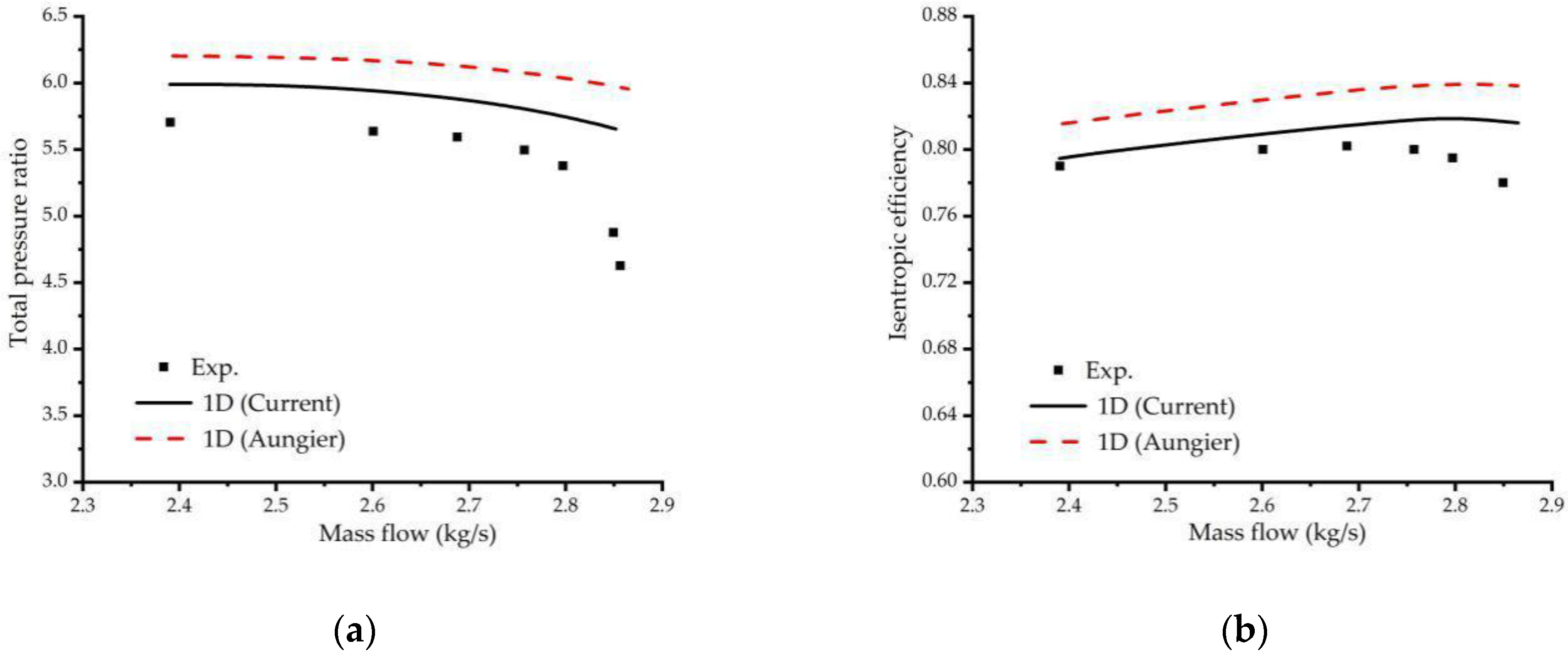
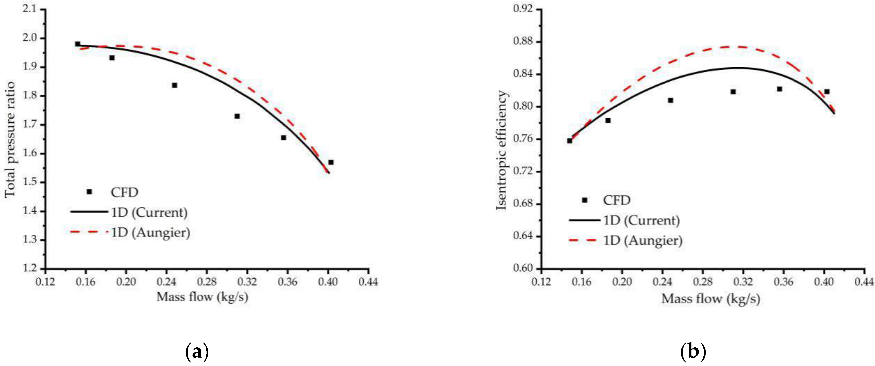
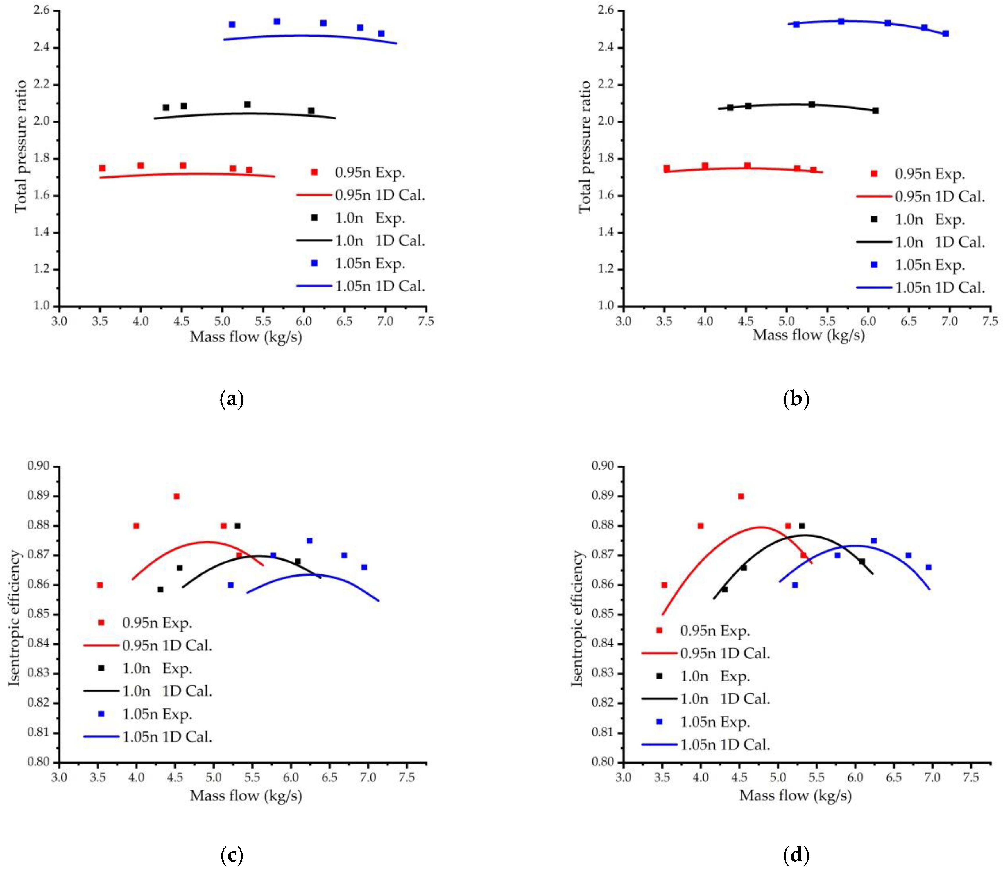
5. Validation of 1D Calculation Method

The aerodynamic performances of the impellers in Table 1 are predicted by using the above introduced 1D method. Through the method in References [11,12], the relatively most optimal loss model set is obtained. The combined models, which can give relatively accurate predictions in our study, are summarized in

Table 2. Loss models and models used in the study.

Component	Loss Models	Proposers	Models Used in This Study
Internal losses	Incidence loss	Galvas, Conrad, Aungier	Galvas
	Skin friction loss	Jansen, Aungier	Jansen
	Blade loading loss	Coppage, Aungier	Coppage
	Tip clearance loss	Jansen, Roders, Krylov and Spunde	Jansen
	Mixing loss	Aлeкceeв, Aungier, Johnston and Dean	Aлeкceeв
	Viscosity loss	Aлeкceeв	Aлeкceeв
	Shock loss	Aungier, Whitfield and Baines, Aлeкceeв	Aлeкceeв
External losses	Disk friction loss	Galvas, Aungier, Daily and Nece, Boyce	Galvas
	Recirculation loss	Aлeкceeв, Roders, Coppage, Oh	Aлeкceeв
	Leakage loss	Aungier, Jansen	Aungier

.

Figure 5, Figure 6, Figure 7 and Figure 8 show the predicted results for three groups of impellers at design speeds. Generally, the selected loss model set has reasonable prediction accuracy for the three groups of impellers in terms of efficiency or total pressure ratio. To further verify the accuracy of the stepping calculation method on the impeller with splitter blades, the widely used Aungier method [6] is used to compare. It can be seen from Figure 6 and Figure 7 that for centrifugal impellers with one row of splitter blades, the predicted results using the stepping calculation method are better than those from the Aungier method. The same result stands for impellers with two rows of splitter blades, as shown in Figure 8 (according to the Formula (28)).

$$\mathit{Z}={\mathit{Z}}_{\mathit{FB}}+{\mathit{Z}}_{\mathit{SB}1}{\mathit{L}}_{\mathit{SB}1}/{\mathit{L}}_{\mathit{FB}}+{\mathit{Z}}_{\mathit{SB}2}{\mathit{L}}_{\mathit{SB}2}/{\mathit{L}}_{\mathit{FB}}$$

(28)

Subscripts 1 and 2 represent the first and second rows of impeller, respectively.

6. Modifications of Coefficients in Loss Models

In order to further improve the accuracy of performance prediction for loss models’ sets selected in Table 2, optimization for loss model coefficients can be conducted. This paper focuses on loss models for impellers. A coefficient f is applied to formulas for each loss model used in the study. Then, a reasonable value range of the coefficients for f is provided, as expressed in Equations (29)–(37).

$$\text{∆}{\mathit{H}}_{\mathit{inc}}={\mathit{f}}_{\mathit{inc}}\frac{{\mathit{W}}_{\mathrm{L}}^2}{2{\mathrm{C}}_{\mathrm{p}}} (0\text{<}{\mathit{f}}_{\mathit{inc}}\text{<}10)$$

(29)

$$\text{∆}{\mathit{H}}_{\mathit{sf}}={{\mathit{f}}_{\mathit{sf}}(5.6\mathit{C}}_{\mathrm{f}}\frac{{\mathit{L}}_{\mathrm{b}}{\mathit{C}}_{2\mathrm{m}}^2}{{\mathit{d}}_{\mathrm{g}}}) (0\text{<}{\mathit{f}}_{\mathit{sf}}\text{<}10)$$

(30)

$$\text{∆}{\mathit{H}}_{\mathit{bl}}={\mathit{f}}_{\mathit{bl}}{(0.05\mathit{D}}_{\mathit{f}}^2{\mathit{u}}_2^2) (0\text{<}{\mathit{f}}_{\mathit{bl}}\text{<}10)$$

(31)

$${\text{∆}\mathit{H}}_{\mathit{cl}}={\mathit{f}}_{\mathit{cl}}{\mathit{C}}_{2\mathit{m}}\frac{3\mathit{\tau }}{5{\mathit{b}}_2}\sqrt{\frac{2\mathit{\pi }{\mathit{C}}_{2\mathit{u}}{\mathit{C}}_{2\mathit{m}}}{\mathit{Z}{\mathit{b}}_2}·\frac{{\mathit{d}}_{1\mathit{t}}^2-{\mathit{d}}_{1\mathit{h}}^2}{\left({\mathit{d}}_{1\mathit{t}}-{\mathit{d}}_{1\mathit{h}}\right)\left(1+\frac{{\mathit{\rho }}_2}{{\mathit{\rho }}_1}\right)}} (0\text{<}{\mathit{f}}_{\mathit{cl}}\text{<}10)$$

(32)

$$\text{∆}{\mathit{H}}_{\mathit{gpr}}={\mathit{f}}_{\mathit{gpr}}\mathit{Work}{\left(1-{\mathit{Re}}_{\mathit{cr}}/1000000\right)}^{2.5} (0\text{<}{\mathit{f}}_{\mathit{gpr}}\text{<}10)$$

(33)

$$\text{∆}{\mathit{H}}_{\mathit{oz}}={\mathit{f}}_{\mathit{oz}}{\mathit{k}}_{\mathrm{z}}{\mathit{t}}_{1\mathit{p}}{\mathit{C}}_{\mathit{p}}\left[{\left(\frac{{\mathit{P}}_{12}}{{\mathit{P}}_{1\mathit{p}}{\mathit{a}}_{\mathit{s}}}\right)}^{\frac{\mathit{k}-1}{\mathit{k}}}-{\left(\frac{{\mathit{P}}_{12}}{{\mathit{P}}_{1\mathit{p}}}\right)}^{\frac{\mathit{k}-1}{\mathit{k}}}\right] (0\text{<}{\mathit{f}}_{\mathit{oz}}\text{<}10)$$

(34)

$$\text{∆}{\mathit{H}}_{\mathit{df}}={\mathit{f}}_{\mathit{df}}\left[{0.01356\mathit{\rho }}_2{{\mathit{d}}_2}^2{\mathit{u}}_2^3/\left(\dot{\mathit{m}}\mathit{R}\mathit{e}\right)\right] (0\text{<}{\mathit{f}}_{\mathit{df}}\text{<}10)$$

(35)

$$\text{∆}{\mathit{H}}_{\mathit{rc}}={\mathit{f}}_{\mathit{rc}}\left(\text{∆}{\mathit{H}}_{\mathit{rc}1}+\text{∆}{\mathit{H}}_{\mathit{rc}2}\right) (0\text{<}{\mathit{f}}_{\mathit{rc}}\text{<}10)$$

(36)

$$\text{∆}{\mathit{H}}_{\mathit{lk}}={\mathit{f}}_{\mathit{lk}}\left\{1.332{\mathit{\rho }}_2\mathit{\epsilon }{\mathit{u}}_2\left[{\mathit{r}}_2{\mathit{C}}_{2\mathit{u}}-{\left({\mathit{r}}_1{\mathit{C}}_{1\mathit{u}}\right)}_{\mathit{m}}\right]/\left(2\stackrel{\mathrm{-}}{\mathit{r}}\stackrel{\mathrm{-}}{\mathit{b}}\right)\right\} (0\text{<}{\mathit{f}}_{\mathit{lk}}\text{<}10)$$

(37)

The Latin hypercube sampling method is employed to establish a sample database of the combination of loss model coefficients in the given range. Then, the efficiency and pressure ratio of the impeller at each sample point are calculated with a Fortran code based on the above introduced 1D analysis method.

The cubic spline function is employed to fit experimental or CFD perdition data for impellers. Afterwards, the functions of mass flow rate to pressure ratio and mass flow rate to efficiency are obtained. The error value Δδ of the efficiency or pressure ratio between the 1D result and the cubic spline function result at each mass flow rate point are obtained by the root-mean-square error function (Equation (38)).

$$\Delta \mathit{\delta }=\sqrt{{\left({\mathit{a}}_{1\mathit{D},1}-{\mathit{a}}_{\mathit{cs},1}\right)}^2+{\left({\mathit{a}}_{1\mathit{D},2}-{\mathit{a}}_{\mathit{cs},2}\right)}^2{+\text{…}+\left({\mathit{a}}_{1\mathit{D},\mathit{i}}-{\mathit{a}}_{\mathit{cs},\mathit{j}}\right)}^2}$$

(38)

where a_1D denotes the 1D predicted total pressure ratio and isentropic efficiency, and a_cs represents the total pressure ratio and isentropic efficiency from the cubic spline function result. Then, the whole error value Δδ of the sample database is obtained according to the above method. The multi-objective genetic algorithm (NSGA-II) is used for optimization. The optimization objective is set as $\Delta \mathit{\delta }$ minimum. Moreover, the final optimization result is acquired by building a Pareto front, so as to construct the optimal loss model coefficients for loss models.

With the Eckardt-O impeller as an example (Figure 9 and

Table 3. Comparison of one-dimensional prediction and fit function results.

Mass Flow	Total Pressure Ratio		Isentropic Efficiency
kg/s	1D Cal.	Cubic spline	1D Cal.	Cubic spline
4.17	2.018	2.071	0.8481	0.8554
4.387	2.027	2.081	0.8542	0.8625
4.814	2.04	2.092	0.8634	0.8725
5.231	2.045	2.094	0.8686	0.8768
5.637	2.043	2.085	0.8699	0.8757
5.836	2.04	2.076	0.8692	0.8731
6.223	2.029	2.052	0.8649	0.8638

), the total pressure ratio error Δε = 0.0938 and the isentropic efficiency error Δη = 0.0145 are calculated through Equation (38). Finally, the optimal coefficients of the loss model combination for Eckardt-O impellers are obtained by building a Pareto front, as exhibited in Figure 10.

7. Optimization Results

7.1. Results for the First Group of Impellers

Figure 11 and Figure 12 show comparisons of 1D predicted performance before and after optimization for the Krain impeller and Eckardt-O impellers, respectively. After the coefficients are optimized, the total pressure ratio error Δε and the isentropic efficiency error Δη are changed from 0.02640 and 0.0088 to 0.00095 and 0.00032 for the Krain impeller at the design speed, respectively. For the Eckardt-O impeller, Δε and Δη are changed from 0.0938 and 0.0145 to 0.000254 and 0.00014 at the design speed, respectively. The results demonstrate that the 1D calculation using the optimized loss models has reasonable prediction accuracy for impellers without splitter blades.

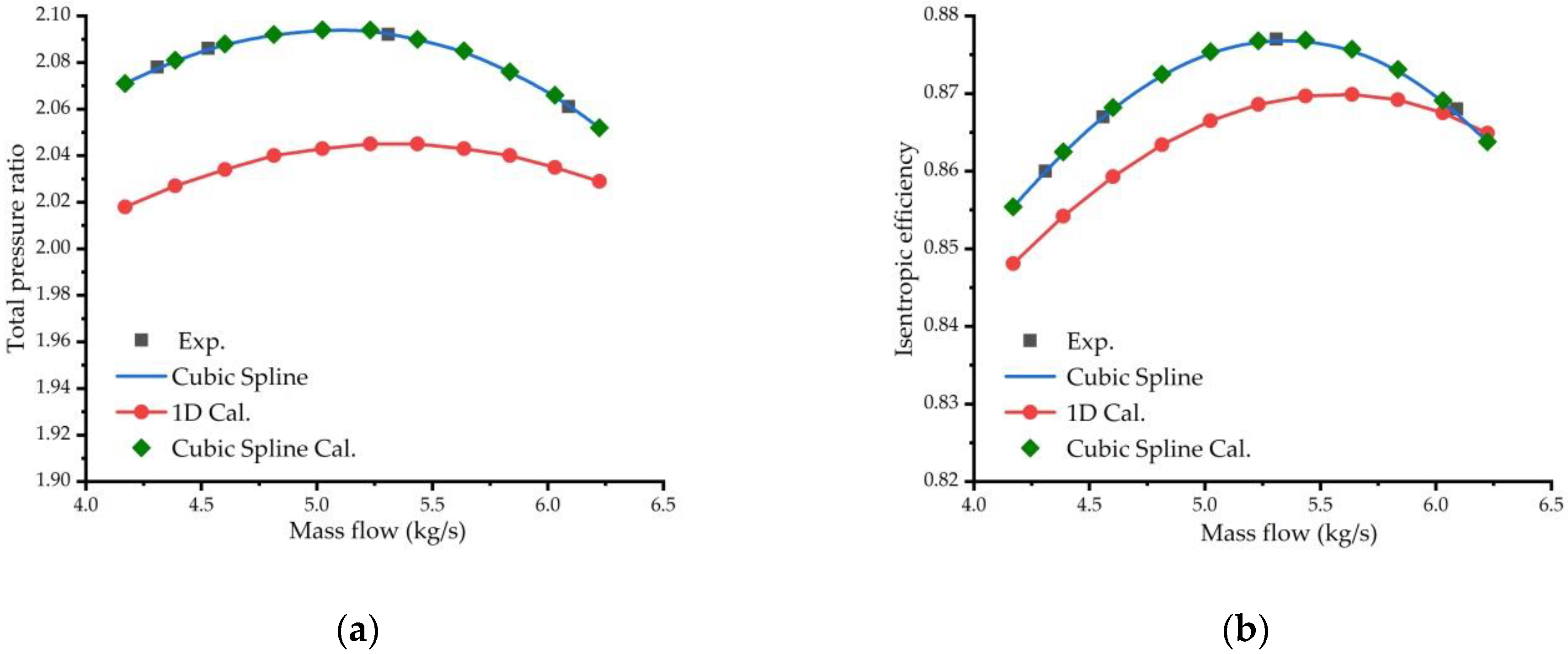
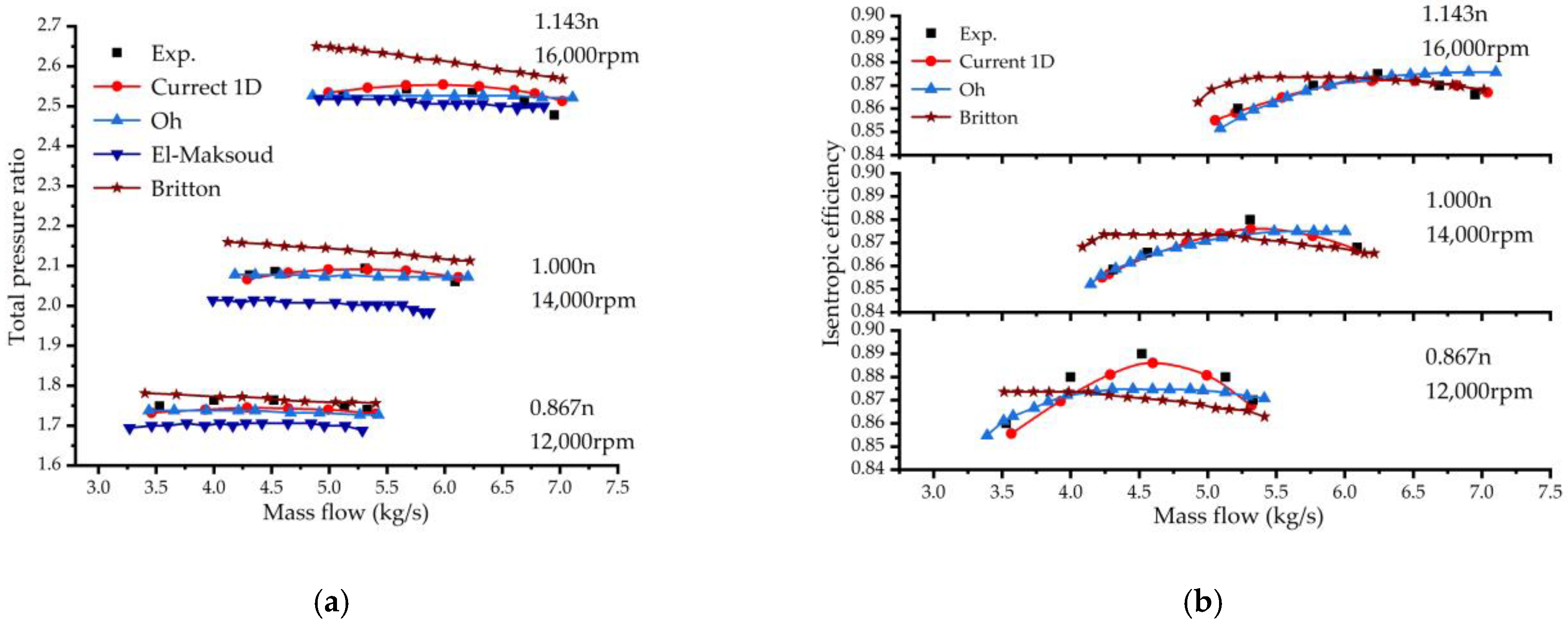
7.2. Comparisons with Other Calculation Methods

The Eckardt-O impeller is cited by a large number of references because its detailed geometric information is available. Here, results of using the single-zone mode from Oh [11] and El-Maksoud [15] and results of using the two-zone model for the Eckardt-O impeller from Britton [38] are selected to compare with the current results. El-Maksoud [15] only provided the predicted pressure ratio results in his paper. As can be seen from Figure 13, the current predicted results are in better agreement with measurements than the other three 1D results. This further demonstrates that the current 1D prediction method has good performance.

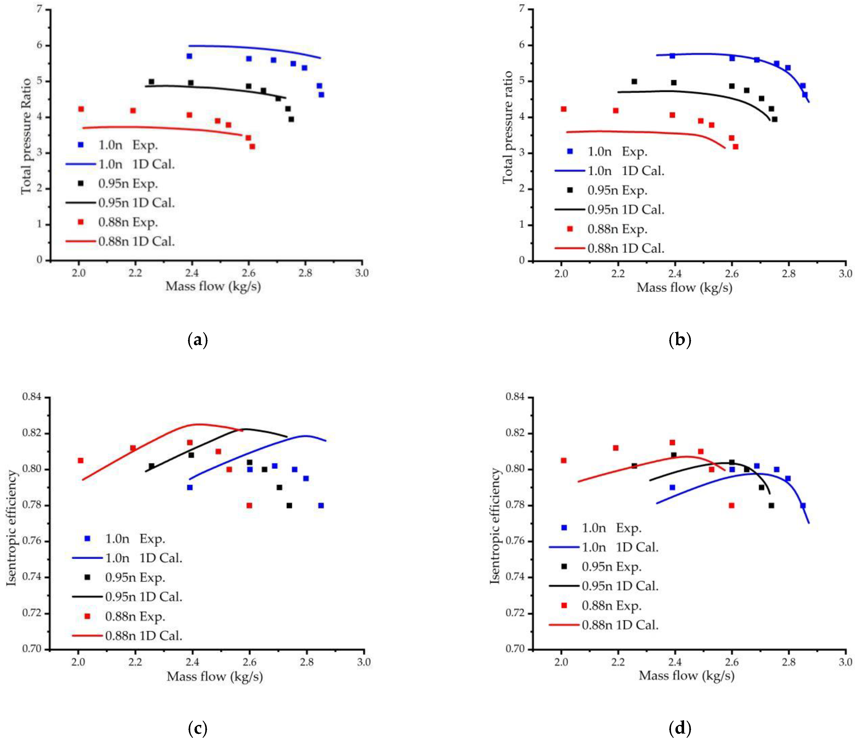
7.3. Results for the Second Group of Impellers

Figure 14 compares 1D predicted performances with measurements and also makes comparisons before and after optimization for the SRV2-O impeller. Figure 15 is for the Impeller R. The impeller R only has the CFD results. After the coefficients in loss models are optimized, the total pressure ratio error Δε and the efficiency error Δη for SRV2-O are changed from 2.1467 and 0.0039 to 0.03891 and 0.00008 in the design speed, respectively. For the impeller R, the total pressure ratio error Δε and the isentropic efficiency error Δη are changed from 0.06528 and 0.00231 to 0.01233 and 0.00005 at the design speed, respectively. It can be revealed that the 1D calculation using the optimized loss models also have reasonable prediction accuracy for the impeller with one row of splitter blades.

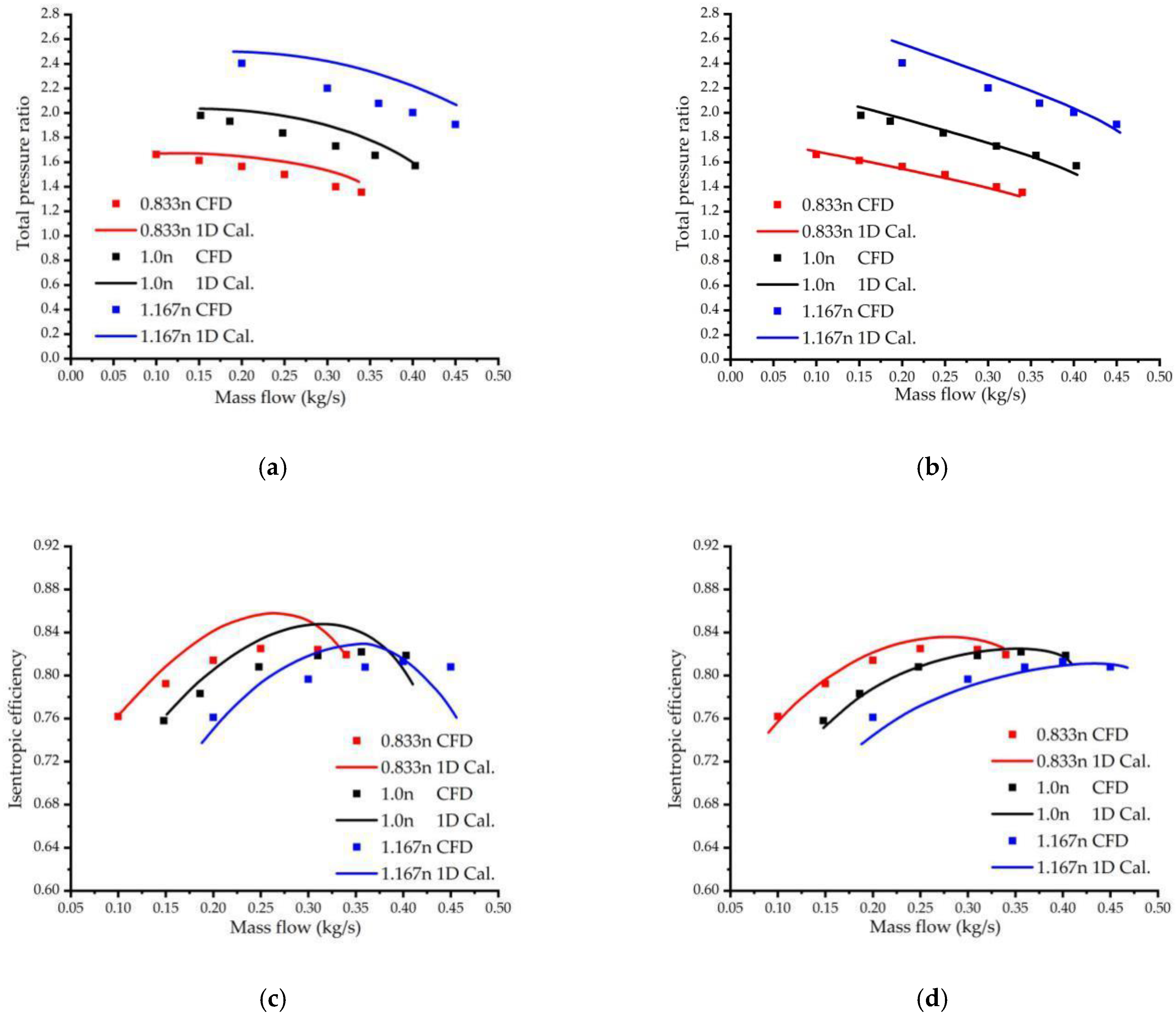
7.4. Results for the Third Group of Impellers

Figure 16 shows performance comparisons before and after optimization of coefficients between 1D and CFD results for Impeller J with two rows of splitter blades. The impeller also only has CFD results. After the coefficients are optimized, the total pressure ratio error Δε and the efficiency error Δη for Impeller J are changed from 0.7389 and 0.003 to 0.0355 and 0.0001 in the design speed, respectively. It can be demonstrated that the modified loss models have good prediction accuracy for the impeller with two rows of splitter blades.

7.5. Value Changes for the Coefficients Involved in the Loss Models

By optimizing the coefficients of loss models’ sets for three groups of impellers, the value changes for the coefficients of the loss models’ set can be recommended and given in

Table 4. Values for coefficients of the loss models’ set after optimization.

Name	finc	fcl	fgpr	fbl	fdf	frc	fsf	foz
Eckardt-O	1.58801	0.4796	4.7907	0.13334	2.93157	2.96052	0.96139
Krain	2.78663	0.5242	2.08658	0.85853	0.14468	0.72164	1.58243
R	1.0772	6.3912	5.2102	4.913	1.6832	0.1231	0.6838
SRV2-O	3.74546	2.07457	3.12488	0.1213	1.32559	0.07233	1.32559	2.63154
J	6.03554	0.81823	3.33042	1.54833	2.84399	0.05061	1.77527	4.84246

. All the original values of the coefficients are 1. It can be seen from the results, the coefficient of incidence loss model increases with the total pressure ratio.

8. Conclusions

The existing 1D analysis method for the impeller with splitter blades is relatively simple and cannot make accurate predictions of aerodynamic performance. To deal with this case, a new single-zone meanline-model prediction method for centrifugal compressors with splitter blades has been proposed in the paper. Modification and optimization of the coefficients involved in loss models has been carried out. Modified loss models have then been verified by using three different types of impellers. The main conclusions can be drawn as follows.

(1)

To reduce the geometric parameters required for calculation, a general meridional channel of the computational domain is established and the calculation method of the leading edge position of the splitter blade is offered. Based on the simplified computational domain, all the geometric parameters required for 1D performance calculations can be obtained.

(2)

Based on the geometric characteristics of impeller with splitter blades, a stepping calculation method is proposed for the impellers with different rows of splitter blades. Along the meridional channel, each section with the same number of blades is treated as an independent impeller. Each sub-impeller can be calculated in turn. Comparisons between predicted aerodynamic performances with experimental data or CFD results for different impellers have demonstrated that the current 1D calculation method is superior to the existing simplified calculation methods.

(3)

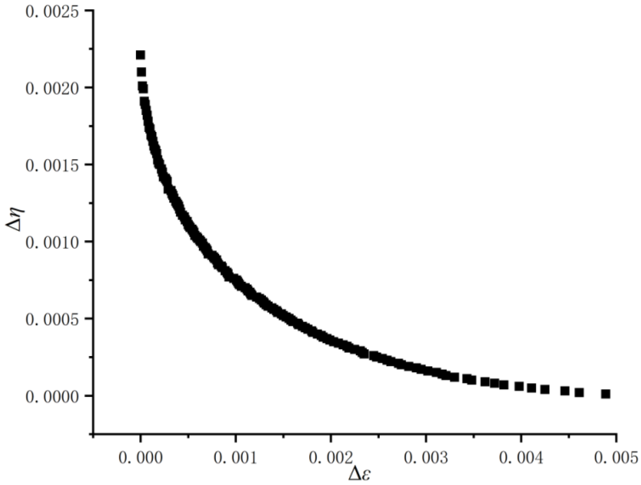
The most optimal loss model set, which is applicable to different types of impellers with different rows, is gained. Coefficients involved in loss models are optimized by using the multi-objective genetic algorithm (NSGA-II). The modified loss models greatly improve the prediction accuracy of the single-zone model. The coefficient optimization method provides a useful tool for improvement in accuracy of loss models.

(4)

In order to further improve the generality of the single-zone model, more impellers with splitter blades will be used for verification in the future.

References

1. Japikse, D. Assessment of Single-and Two-Zone Modeling of Centrifugal Compressors, Studies in Component Performance: Part 3; American Society of Mechanical Engineers: New York, NY, USA, 1985; Volume 79382, p. V001T003A023. [Google Scholar]
2. Aungier, R.H.X. Mean streamline aerodynamic performance analysis of centrifugal compressors. J. Turbomach. 1995, 117, 360–366. [Google Scholar] [CrossRef]
3. Cicciotti, M.; Martinez-Botas, R.; Gozalbo, R.; Geist, S.; Schild, A.; Thornhill, N.F.; Khars, O.; Reiser, W. Assessment of meanline models for centrifugal compressors in the process plant industry. In Proceedings of the 5th International Symposium on Fluid Machinery and Fluids Engineering (ISFMFE), Jeju, Republic of Korea, 24–27 October 2012. [Google Scholar]
4. Cicciotti, M.; Martinez-Botas, R.F.; Romagnoli, A.; Thornhill, N.F.; Geist, S.; Schild, A. Systematic One Zone Meanline Modelling of Centrifugal Compressors for Industrial Online Applications; American Society of Mechanical Engineers: New York, NY, USA, 2013; Volume 55249, p. V06CT40A025. [Google Scholar]
5. VeláSquez, E.I.G. Determination of a suitable set of loss models for centrifugal compressor performance prediction. Chin. J. Aeronaut. 2017, 30, 1644–1650. [Google Scholar] [CrossRef]
6. Galvas, M.R. Fortran Program for Predicting Off-Design Performance of Centrifugal Compressors; National Aeronautics and Space Administration: Washington, DC, USA, 1973.
7. Aungier, R.H.X. Centrifugal Compressors: A Strategy for Aerodynamic Design and Analysis; American Society of Mechanical Engineers Press: New York, NY, USA, 2000. [Google Scholar]
8. Whitfield, A.; Baines, N.C. Design of Radial Turbomachines; Longman: London, UK, 1990. [Google Scholar]
9. Li, P.-Y.; Gu, C.-W.; Song, Y. A new optimization method for centrifugal compressors based on 1D calculations and analyses. Energies 2015, 8, 4317–4334. [Google Scholar] [CrossRef]
10. Sundström, E.; Kerres, B.; Sanz, S.; Mihăescu, M. On the Assessment of Centrifugal Compressor Performance Parameters by Theoretical and Computational Models; American Society of Mechanical Engineers: New York, NY, USA, 2017; Volume 50800, p. V02CT44A029. [Google Scholar]
11. Oh, H.W.; Yoon, E.S.; Chung, M.K. An optimum set of loss models for performance prediction of centrifugal compressors. Proc. Inst. Mech. Eng. Part A J. Power Energy 1997, 211, 331–338. [Google Scholar] [CrossRef]
12. Zhang, C.; Dong, X.; Liu, X.; Sun, Z.; Wu, S.; Gao, Q.; Tan, C. A method to select loss correlations for centrifugal compressor performance prediction. Aerosp. Sci. Technol. 2019, 93, 105335. [Google Scholar] [CrossRef]
13. Harley, P.; Spence, S.; Filsinger, D.; Dietrich, M.; Early, J. Assessing 1D Loss Models for the Off-Design Performance Prediction of Automotive Turbocharger Compressors; American Society of Mechanical Engineers: New York, NY, USA, 2013; Volume 55249, p. V06CT40A005. [Google Scholar]
14. Du, W.; Li, Y.; Li, L.; Lorenzini, G. A quasi-one-dimensional model for the centrifugal compressors performance simulations. Int. J. Heat Technol. 2018, 36, 391–396. [Google Scholar] [CrossRef]
15. Abd El-Maksoud, R.M.; Bayomi, N.N.; Rezk, M.I.F. Prediction and Modification of Centrifugal Compressor Performance Maps. In Proceedings of the Al-Azhar Engineering Twelfth International Conference, Cairo, Egypt, 25–27 December 2012. [Google Scholar]
16. Jiang, H.; Dong, S.; Liu, Z.; He, Y.; Ai, F. Performance prediction of the centrifugal compressor based on a limited number of sample data. Math. Probl. Eng. 2019, 2019, 5954128. [Google Scholar] [CrossRef] [Green Version]
17. Bourabia, L.; Abed, C.B.; Cerdoun, M.; Khalfallah, S.; Deligant, M.; Khelladi, S.; Chettibi, T. Aerodynamic preliminary design optimization of a centrifugal compressor turbocharger based on one-dimensional mean-line model. Eng. Comput. 2021, 38, 3438–3469. [Google Scholar] [CrossRef]
18. Massoudi, S.; Picard, C.; Schiffmann, J. Robust design using multiobjective optimisation and artificial neural networks with application to a heat pump radial compressor. Des. Sci. 2022, 8, e1. [Google Scholar] [CrossRef]
19. Bicchi, M.; Biliotti, D.; Marconcini, M.; Toni, L.; Cangioli, F.; Arnone, A. An AI-Based Fast Design Method for New Centrifugal Compressor Families. Machines 2022, 10, 458. [Google Scholar] [CrossRef]
20. Du, Y.; Yang, C.; Wang, H.; Hu, C. One-dimensional optimisation design and off-design operation strategy of centrifugal compressor for supercritical carbon dioxide Brayton cycle. Appl. Therm. Eng. 2021, 196, 117318. [Google Scholar] [CrossRef]
21. Romei, A.; Gaetani, P.; Giostri, A.; Persico, G. The role of turbomachinery performance in the optimization of supercritical carbon dioxide power systems. J. Turbomach. 2020, 142, 071001. [Google Scholar] [CrossRef]
22. Wang, J.; Guo, Y.; Zhou, K.; Xia, J.; Li, Y.; Zhao, P.; Dai, Y. Design and performance analysis of compressor and turbine in supercritical CO2 power cycle based on system-component coupled optimization. Energy Convers. Manag. 2020, 221, 113179. [Google Scholar] [CrossRef]
23. Conrad, O.; Raif, K.; Wessels, M. The calculation of performance maps for centrifugal compressors with vane-island diffusers. In Performance Prediction of Centrifugal Pumps and Compressors; American Society of Mechanical Engineers: New York, NY, USA, 1979; pp. 135–147. [Google Scholar]
24. Jansen, W. A method for calculating the flow in a centrifugal impeller when entropy gradient are present. Inst. Mech. Eng. Intern. Aerodyn. 1970, 133–146. Available online: https://cir.nii.ac.jp/crid/1571135650145571968 (accessed on 10 October 2022).
25. Coppage, J.E.; Dallenbach, F. Study of Supersonic Radial Compressors for Refrigeration and Pressurization Systems; Garrett Corp Los Angeles Ca AiResearch MFG DIV: Los Angeles, CA, USA, 1956. [Google Scholar]
26. Rodgers, C. Paper 5: A Cycle Analysis Technique for Small Gas Turbines; SAGE Publications Sage UK: London, UK, 1968; Volume 183, pp. 37–49. [Google Scholar]
27. Krylov, E.P.; Spunde, Y.A. About the Influence of the Clearance between the Working Blades and Housing of a Radial Turbine on Its Exponent; Air Force Systems Command Wright-Patterson AFB Oh Wright-Patterson AFB: Dayton, OH, USA, 1967. [Google Scholar]
28. Алексеев. Принцип авиациoнных двигателей; Издательствo науки и правды: Volgogrd, Soviet Union, 1982. [Google Scholar]
29. Johnston, J.P.; Dean, R.C., Jr. Losses in vaneless diffusers of centrifugal compressors and pumps: Analysis, experiment, and design. J. Eng. Power. 1966, 88, 49–60. [Google Scholar] [CrossRef]
30. Daily, J.W.; Nece, R.E. Chamber dimension effects on induced flow and frictional resistance of enclosed rotating disks. J. Basic Eng. 1960, 82, 217–230. [Google Scholar] [CrossRef]
31. Boyce, M.P. Centrifugal Compressors: A Basic Guide; PennWell Corporation: Tulsa, OK, USA, 2003. [Google Scholar]
32. Stanitz, J.D. One-Dimensional Compressible Flow in Vaneless Diffusers of Radial-and Mixed-Flow Centrifugal Compressors, Including Effects of Friction, Heat Transfer and Area Change; National Advisory Committee for Aeronautics: Washington, DC, USA, 1952.
33. Deb, K.; Agrawal, S.; Pratap, A.; Meyarivan, T. A Fast Elitist Non-Dominated Sorting Genetic Algorithm for Multi-Objective Optimization: NSGA-II; Springer: Berlin/Heidelberg, Germany, 2000; pp. 849–858. [Google Scholar]
34. Krain, H.; Hoffmann, B.; Pak, H. Aerodynamics of a Centrifugal Compressor Impeller with Transonic Inlet Conditions; American Society of Mechanical Engineers: New York, NY, USA, 1995; Volume 78781, p. V001T001A011. [Google Scholar]
35. Eckardt, D. Instantaneous measurements in the jet-wake discharge flow of a centrifugal compressor impeller. J. Eng. Gas Turbines Power 1975, 97, 337–345. [Google Scholar] [CrossRef]
36. Moore, J. Eckardt’s impeller: A ghost from ages past. NASA STI/Recon Tech. Rep. N 1976, 77, 28442. [Google Scholar]
37. Eisenlohr, G.; Krain, H.; Richter, F.-A.; Tiede, V. Investigations of the flow through a high pressure ratio centrifugal impeller. In Proceedings of the Turbo Expo: Power for Land, Sea, and Air, Amsterdam, The Netherlands, 3–6 June 2002; Volume 3610, pp. 649–657. [Google Scholar]
38. Britton, I.; Gauthier, J.E.D. Performance prediction of centrifugal impellers using a two-zone model. In Proceedings of the Turbo Expo: Power for Land, Sea, and Air, Berlin, Germany, 9–13 June 2008; Volume 43161, pp. 1695–1704. [Google Scholar]
Figure 1. Meridional channel of the computational domain.
Machines 11 00118 g001
Figure 2. Different types of impellers: (a) Impeller without splitter blades; (b) Impeller with one row of splitter blades; (c) Impeller with two rows of splitter blades.
Machines 11 00118 g002
Figure 3. Decomposition of the impeller with splitter blades: (a) Impeller with one row of splitter blades; (b) Impeller with two rows of splitter blades.
Machines 11 00118 g003
Figure 4. Aerodynamic calculation process for an impeller with splitter blades.
Machines 11 00118 g004
Figure 5. Performance comparison for: (a) Krain impeller; (b) Eckardt-O impeller.
Machines 11 00118 g005
Figure 6. Performance comparison for two methods for the SRV2-O impeller: (a) Total pressure ratio; (b) Isentropic efficiency.
Machines 11 00118 g006
Figure 7. Performance comparison for two methods for Impeller R: (a) Total pressure ratio; (b) Isentropic efficiency.
Machines 11 00118 g007
Figure 8. Performance comparison for two methods for Impeller J: (a) Total pressure ratio; (b) Isentropic efficiency.
Machines 11 00118 g008
Figure 9. Eckardt-O performance comparison: (a) Total pressure ratio comparison; (b) Efficiency comparison.
Machines 11 00118 g009
Figure 10. Pareto front for the Eckardt-O impeller.
Machines 11 00118 g010
Figure 11. Comparisons of 1D predicted performance before and after optimization for the Krain impeller: (a) Total pressure ratio before optimization; (b) Total pressure ratio after optimization; (c) Efficiency before optimization; (d) Efficiency after optimization.
Machines 11 00118 g011
Figure 12. Comparisons of the 1D predicted performance before and after optimization for the Eckardt-O impeller: (a) Total pressure ratio before optimization; (b) Total pressure ratio after optimization; (c) Efficiency before optimization; (d) Efficiency after optimization.
Machines 11 00118 g012
Figure 13. Comparisons of different 1D prediction for the Eckardt-O impeller: (a) Total pressure ratio; (b) Isentropic efficiency.
Machines 11 00118 g013
Figure 14. Comparisons of the 1D predicted performance before and after optimization for the SRV2-O impeller: (a) Total pressure ratio before optimization; (b) Total pressure ratio after optimization; (c) Efficiency before optimization; (d) Efficiency after optimization.
Machines 11 00118 g014
Figure 15. Comparisons of the 1D predicted performance before and after optimization for the R impeller: (a) Total pressure ratio before optimization; (b) Total pressure ratio after optimization; (c) Efficiency before optimization; (d) Efficiency after optimization.
Machines 11 00118 g015
Figure 16. Comparisons of the 1D predicted performance before and after optimization for the impeller J: (a) Total pressure ratio before optimization; (b) Total pressure ratio after optimization; (c) Efficiency before optimization; (d) Efficiency after optimization.
Machines 11 00118 g016