Online Cartesian Compliance Shaping of Redundant Robots in Assembly Tasks

Abstract

This paper presents a universal approach to shaping the mechanical properties of the interaction between a collaborative robot and its environment through an end-effector Cartesian compliance shaping. More specifically, the focus is on the class of kinematically redundant robots, for which a novel redundancy reconfiguration scheme for online optimization of the Cartesian compliance of the end-effector is presented. The null-space reconfiguration aims to enable the more efficient and versatile use of collaborative robots, including robots with passive compliant joints. The proposed approach is model-based and gradient-based to enable real-time computation and reconfiguration of the robot for Cartesian compliance while ensuring accurate position tracking. The optimization algorithm combines two coordinate frames: the global (world) coordinate frame commonly used for end-effector trajectory tracking; and the coordinate frame fixed to the end-effector in which optimization is computed. Another attractive feature of the approach is the bound on the magnitude of the interaction force in contact tasks. The results are validated on a torque-controlled 7-DOF KUKA LWR robot emulating joint compliance in a quasi-static experiment (the robot exerts a force on an external object) and a peg-in-hole experiment emulating an assembly task.

1. Introduction

We face numerous global challenges that require the use of robots in areas where they have never been used before. The COVID-19 pandemic underscores the need for a wider use of robots [1] in production lines, everyday service tasks, and especially in hospitals to directly support healthcare providers and patients or for rehabilitation and intervention purposes.

In all of the above cases, robots must work with or near humans. Therefore, safety measures must be considered to ensure safe but efficient physical human–robot interaction (pHRI) [2]. A safe pHRI is achieved through end-effector (EE) compliance. EE compliance is the ability of the robot’s EE to make displacements from the equilibrium position while an interaction force is applied. Compliance can be achieved in two ways: (1) passive compliance: technology where elastic elements are embedded between the link side and the actuator side; and (2) active compliance: compliant behavior is achieved with a control loop based on force/torque measurements. The use of flexible mechanical joints (passive compliance) [3,4] and complementary active compliance technologies [5,6,7] has led to the development of modern collaborative robots [8,9]. Modern collaborative robots can enable safe interaction through compliant joints without additional safety hardware (e.g., laser curtains or mechanical guards), which reduces the required space [10]. However, for such robots to remain versatile, new tools and methods must be developed that can utilize compliant joints [11]. Thus, in this paper, we propose a framework for a novel redundancy resolution scheme for fast online optimization of Cartesian stiffness for collaborative robots.

Previous works. The typical approach to shaping the EE Cartesian stiffness is active control, where the EE stiffness matrix is adjusted by controlling the joint torques of a rigid-joint robot [12,13]. One of the shortcomings of active control for rigid-joint robots is a high force amplitude reaction in the case of a collision with the environment since the controller cannot react immediately. This problem is partly solved by using compliant actuators, which introduce elasticity between the actuator and the robot joint [4]. EE Cartesian stiffness shaping of a kinematically redundant robot with passive joint stiffness could be considered as a two-part optimization problem [14]: (i) fast (linear) optimization in the space of joint stiffness values, where linearity is achieved by selecting an appropriate optimization norm; and (ii) slow (nonlinear) optimization into the null space of the robot, which can be computed only offline, in the planning phase for the working posture. Furthermore, according to Ref. [15], the two complementary approaches to EE compliance shaping for VSA-driven robots are defined and referred to as (i) configuration-dependent stiffness (CDS)—redundancy is exploited to achieve desired EE stiffness ellipsoid shape, and (ii) common-mode stiffness (CMS)—the CMS is an additional control parameter that linearly scales all joint stiffness and thus linearly scales the EE stiffness. The approach from [14] and one that combines passive and active stiffness for better performance [16] deals with the control of all six EE coordinates (three positions and three orientations) and 21 different elements in the full $6\times 6$ EE symmetric stiffness matrix. This results in 27 variables. Therefore, the control design in this multi-variable non-linear coupled space is very challenging due to many variables and physical constraints (limited range of joint motion and stiffness) and few control inputs. Lack of degree of redundancy could lead to poor performance in shaping EE stiffness [17]. However, as shown in [18], the control of the diagonal elements of the stiffness matrix is essential in most applications. Additionally, control of the EE stiffness of VSA-driven robots can be achieved by extending the redundant inverse kinematics problem to include variable compliance in each joint [19]. Ref. [20] presents an algorithm that shapes the impedances according to constrained task dynamics along/about specific directions while computing stiffness and damping for optimal EE impedance planning is discussed in [21]. Both of these papers address robots with active compliance and do not consider robots with constant (passive) joint stiffness. Several null-space controllers for EE compliance shaping developed in [22,23,24,25] aim at robots with active compliance, while the research proposed in this paper has broader usage. In our research, the active compliance KUKA LWR robot was used as a research platform without limiting our results only to active compliance robots. Thus, this paper presents a control framework that can be applied to robots with active compliance and robots with passive compliance. One of the most significant contributions is for redundant robots driven with constant passive compliance that cannot be changed, but all EE stiffness shaping has to be done in null space.

Paper Contributions. In this paper, we present a novel computationally efficient model-based EE compliance shaping for robots with constant joint stiffness while maintaining trajectory tracking performance. The EE compliance of the robot is adjusted through null-space projection as originally introduced by the authors of the present paper in [26]. An important technical aspect of the presented research is related to online computation during the execution of the task, in contrast to most of the results available in the literature that consider only the static pose of the robot. Typically, a 7 DOF robot has very few degrees of redundancy, so it is not possible to control all elements of the EE stiffness/compliance matrix. Therefore, the research presented in this paper mainly focuses on the design of task-relevant stiffness along the axis of movement. The proposed solution was experimentally validated in a peg-in-hole task on the KUKA LWR robot. It showed that appropriate modulation of the stiffness along the motion axis could improve the performance of the task.

Paper structure: Section 2 presents the main contribution of the paper. It summarizes the theoretical background for the implementation of inverse kinematics with the secondary task of shaping EE compliance, followed by a stability analysis of the control algorithm. Section 3 explains the implementation of the algorithm, and Section 4 presents experimental results on the KUKA LWR robot to validate the algorithm. Section 5 contains the discussion, while conclusions are provided in Section 6.

2. Null-Space Projection Shaping Approach

It is known that the Cartesian stiffness of EE (given by the matrix $K_C$) depends on the stiffness of the individual joints (given by the matrix $K_j$) and the robot configuration, which is reflected in the Jacobian matrix $J$ that maps joint velocities to EE velocities. This relationship between joint stiffness and Cartesian stiffness is explained in more detail in [14] and [16] and is given by

$$K_C={\left(J\left(q\right)K_j^{-1}J{\left(q\right)}^T\right)}^{-1},$$

(1)

whereas the relationship between the EE Cartesian compliance matrix $C_C$ and the joint stiffness matrix $K_j$ is represented in the less computationally demanding form as follows

$$C_C=J\left(q\right)K_j^{-1}J{\left(q\right)}^T.$$

(2)

Here, $K_C$ ($C_C$) is the symmetric $m\times m$ Cartesian stiffness (compliance) matrix, $K_j$ is the $n\times n$ diagonal joint stiffness matrix, $J$ is the $m\times n$ Jacobian matrix, and $q$ is the $n$-dimensional joint position vector. The parameters $m$ and $n$ are the dimensions of the task and the joint space, respectively.

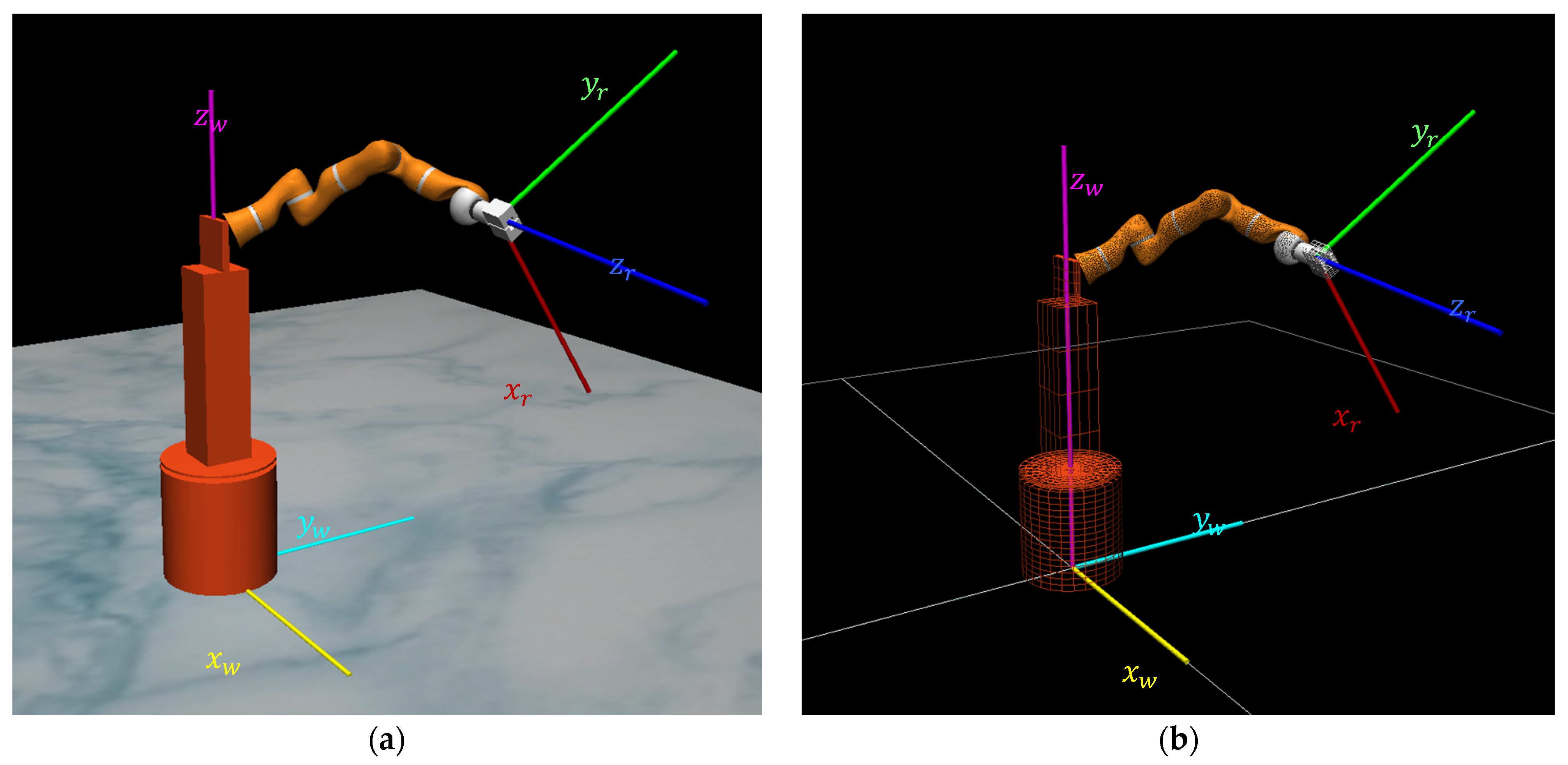
For the robot shown in Figure 1, the EE Cartesian position ($X_w$), orientation ($R_w$), and Jacobian matrix ($J_w$) in a world frame are defined in [27] as

$$X_w=R_p{X}_r+X_p,$$

(3)

$$R_w=R_p{R}_r,$$

(4)

$$J_w=\left[\begin{array}{cc}{R}_p& \mathit{O}\\ \mathit{O}& R_p\end{array}\right]J,$$

(5)

where $\mathit{O}$ is the zero matrix of appropriate dimension.

The Euler angles for the EE orientation $\varphi , \psi ,$ and $\theta$ in the world frame are extracted from the orientation matrix $R_w$. Therefore, the EE position vector in the world frame is defined as $X={\left[x,y,z,\varphi , \psi , \theta \right]}^T$. The platform position offset and the rotation matrix with respect to the world frame are denoted by $X_p$ and $R_p$, respectively, whereas $X_r$ and $R_r$ are the robot EE position and orientation matrices corresponding to the robot base coordinate frame, respectively.

To obtain a mathematical model of the EE compliance behavior in the EE frame, it is necessary to compute the Jacobian matrix in EE the frame ($J_{EE}$) as

$$J_{EE}=\left[\begin{array}{cc}{R}_r^T& \mathit{O}\\ \mathit{O}& R_r^T\end{array}\right]J.$$

(6)

By adopting the Jacobian from (6) and substituting it in (2), the expression for compliance in the EE frame, $C_{EE}$, becomes

$$C_{EE}=J_{EE}{K}_j^{-1} J_{EE}^T.$$

(7)

The stiffness in the EE frame, $K_{EE}$, is computed as

$$K_{EE}=C_{EE}^{-1}.$$

(8)

An illustration of the world frame and the EE frame coordinate systems is depicted in Figure 1.

The general norm ($H_c$) for the robot’s EE Cartesian compliance shaping, which is the measure of how close the achieved compliance is to the desired compliance, can be defined as follows

$$H_c=\Vert C_{CD}-C_{CEE}\left(q\right)\Vert ,$$

(9)

where $C_{CD}$ is the desired compliance and $C_{CEE}$ is the achieved compliance in the EE frame.

The challenge of adjusting Cartesian compliance while moving along a defined path can be observed as the minimization of $H_c$. One of the computational approaches to the norm $H_c$ defined in general form (9) is Euclidean norm in combination with a weighted matrix to have the form as

$$H_c={\displaystyle \sum }_{i,j}{W}_{ij}{\left(C_{C{D}_{ij}}-C_{CEE}{\left(q\right)}_{ij} \right)}^2,$$

(10)

where $W$ is the $m\times m$ weighted matrix and $i$ and $j$ denote the elements of the corresponding matrix. The role of the weighted matrix is to prioritize some elements over others when multiple elements are shaped simultaneously, considering that there are enough degrees of redundancy. Prioritization of particular axes is essential when only a few degrees of redundancy are available, meaning that very few elements within the EE compliance matrix can be adjusted. Usually, the weighted matrix is chosen to optimize compliance according to the requirements of the task.

For a redundant robot, a general solution to the inverse kinematics [28] is described as

$$\dot{q}=J_w^{†}\dot{X}+\left(I_n-J_w^{†}{J}_w\right){\dot{q}}_N$$

(11)

where $\dot{X}$ is the EE velocity vector in the world frame, ${\dot{q}}_{\mathrm{N}}$ is an arbitrary joint-space velocity, $I_n$ is the $n$-dimensional identity matrix, and $J_w^{†}$ is the general pseudo-inverse of $J_w.$ The Moore–Penrose pseudo-inverse will be used hereafter, defined as $J_w^{†}=J_w^T{\left(J_w{J}_w^T\right)}^{-1}$ [29], where $J_w{J}_w^{†}=I$.

For kinematically redundant robots, the arbitrary joint space velocity ${\dot{q}}_N$ can be computed to perform a secondary task. In the present case, the secondary task can be the minimization of the norm given in (10). Since the secondary task is to minimize the norm $H_c$, joint velocity ${\dot{q}}_N$ is calculated using the gradient of $H_c$ [28]

$${\dot{q}}_N=K_n\nabla H_c\left(q\right),$$

(12)

where $K_n$ is the diagonal gain matrix with positive values on the main diagonal and $\nabla H_c\left(q\right)$ is the gradient of $H_c$. The inverse kinematic Cartesian controller at the velocity level is given by

$$\dot{X}=K\left(X_d-X\right),$$

(13)

where $K$ is the diagonal gain matrix with positive values on the main diagonal and $X_d$ is the commanded Cartesian position.

A Cartesian controller with Cartesian stiffness matrix shaping is obtained by substituting (12) and (13) into (11),

$$\dot{q}=J_w^{†} K\left(X_d-X\right)+\left(I_n-J_w^{†}{J}_w\right)K_n\nabla H_c\left(q\right).$$

(14)

The controller obtained in (14) has two functions: (1) the first addition ($J_w^{†} K\left(X_d-X\right)$) secures trajectory tracking performance in the world frame; and (2) the second addition ($\left(I_n-J_w^{†}{J}_w\right)K_n\nabla H_c\left(q\right)$) secure EE stiffness shaping in the EE frame while keeping the influence of the first addition unchanged.

The desired joint positions $q_d$ are computed as

$$q_d=q_0+\int \dot{q}dt,$$

(15)

where $q_0$ is the $n$-dimensional vector of initial joint positions. By substituting (14) into (15), the final expression for the desired joint positions $q_d$ is

$$q_d=q_0+\int \left(J_w^{†} K\left(X_d-X\right)+\left(I_n-J_w^{†}{J}_w\right)K_n\nabla H_c\left(q\right)\right)dt.$$

(16)

The proposed gradient-based null-space control algorithm guarantees the stability of the algorithm and smooth position trajectories while adjusting the compliance of EE in an arbitrary direction. The proof of stability for the algorithm can be found in Appendix A.

3. Algorithm Implementation

The proposed algorithm was validated on the KUKA LWR robot arm with actively controlled compliant joints. To validate the approach, joint compliance was emulated with PD torque control at the joint level. Joint torques $\tau$ were computed as

$$\tau =K_p\left(q_d-q\right)+K_d\left({\dot{q}}_d-\dot{q}\right)+g\left(q\right),$$

(17)

where $K_p$ and $K_d$ are gains (diagonal gain matrix with positive values on the main diagonal) of the torque PD controller and $g\left(q\right)$ is the gravity compensation term. Proportional gain is a diagonal matrix whose values correspond to the desired joint stiffness values, $K_p=K_j.$ The differential gain matrix, $K_d$, corresponds to joint damping, which reduces joint oscillations as $K_d=2\sqrt{K_p}$. The gain magnitudes, $K_p$ and $K_d$, are tuned according to the values of the joint stiffness matrix, $K_j$. The gravity compensation is obtained from KUKA’s Fast Robot Interface (FRI).

The desired position vector $q_d$ was numerically computed in two steps. In the first step, the gradient $\nabla H_c$ was numerically obtained as $\nabla {\widehat{H}}_c$

$$\nabla {\widehat{H}}_c\left(q\right)={\left[\nabla {\widehat{H}}_1 \nabla {\widehat{H}}_2 \nabla {\widehat{H}}_3 \nabla {\widehat{H}}_4 \nabla {\widehat{H}}_5 \nabla {\widehat{H}}_6\nabla {\widehat{H}}_7\right]}^T,$$

(18)

where

$$\nabla {\widehat{H}}_i=\frac{H_c\left(q+\Delta q_i\right)-H_c\left(q\right)}{ϵ}, i=1\dots 7$$

(19)

$$\Delta q_{j,i}=\left\{\begin{array}{ll}0& i\ne j\\ ϵ& i=j\end{array}\right., i,j=1\dots 7$$

$ϵ$ was a small enough constant required to numerically compute the gradient $\nabla H$, where the norm $H_c$ is computed according to Equation (10) when the weight element is omitted. The $\Delta q_i$ is the $i$-th column of the diagonal matrix $\Delta q$. In the second step, joint velocity was computed using control (14) and the desired joint position $q_{k+1}$ from (18) and (19) in a discrete space:

$$q_{k+1}=q_k+\dot{q} \Delta t,$$

(20)

where $\Delta t$ is the sample period in the control loop.

The algorithm implementation structure of the proposed optimization algorithm is given in Figure 2.

4. Experiment Results

The proposed method was validated in a static experiment (steady state after collision) and a peg-in-hole experiment, simulating an assembly task. In the static experiment, the robot interacted with a compliant environment, i.e., pushing the sponge, which created an interaction force. The interaction force prevented the robot EE from reaching the desired position within the sponge. In the peg-in-hole experiment, the goal of the robot was to place the peg into a mold as smoothly as possible while avoiding high interaction forces. This was achieved by the EE varying the compliance of the robot along the direction of motion. The experiment emulated a typical assembly task where the interaction force was generated by the interaction between an object in the gripper and the environment. The parameters of the robot platform can be found in [30]. All values for joint stiffness were set to 400 Nm/rad. The gain parameters, $K_p$ and $K_d$, were set as diagonal matrices with all values equal and set to 400 Nm/rad and 40 Nms/rad, respectively. The inverse kinematic control parameters, $K$ and $K_n$, were diagonal matrices with all values equal and set to 10 and 1, respectively. The parameter for the numerical calculation of the gradient was $\Delta q={10}^{-7}$ rad, and the control loop interval was set to $\Delta t=0.01$ s.

4.1. Validation: End-Effector in Contact with a Soft Surface

The method was applied in a static experiment that also allowed visual validation. For better illustration, the compliance of the EE along the direction of motion was set to the smallest or largest possible value without losing generality. Since there was only one degree of redundancy, the compliance shaping stopped when one of the joints reached its limit or a local minimum for the norm $H_c$ was reached. The experiment is shown in Figure 3, which illustrates EE contact with a surface. In this experiment, the robot’s EE moved downward toward the sponge, with its endpoint reference 5 cm into the area of the sponge. Then the EE adjusted its stiffness. This was repeated to minimize and maximize the stiffness along the $z$-axis. The effect of adjusting the stiffness on the EE is shown by comparing the two images at the end of the shaping algorithm in Figure 3, and the measurements are shown in Figure 4. The ability to adjust the stiffness is also limited to the pose of the robot. When the robot is positioned at the end of its range, there is less maneuverability than in the middle of the workspace. The results showed that there was a strong correlation between the estimated and expected stiffness of the EE. The estimated stiffness was slightly higher than the theoretical. Nevertheless, these values had a high level of correlation. Videos of the sponge experiments are available as Supplementary Materials.

4.2. Peg-In-Hole Example

The peg-in-hole experiment emulated a typical assembly task. The robot’s goal was to put a peg into the mold as smoothly as possible while adjusting EE compliance and avoiding high interaction forces as discussed in [31,32]. This was accomplished by having the EE change the compliance of the robot along the direction of motion. The peg was attached to the gripper of the robot and the mold was clamped to a table. The length of the gripper with the peg was 20 cm. In this experiment, the compliance was adjusted along the vertical axis of the peg, i.e., the z-axis.

The path in the Cartesian space was recorded using kinaesthetic teaching [33]. The recorded sequence is shown in Figure 5. The steps of the EE trajectory can be divided into stages [32]: (1) initial stage (initial position—Figure 5a); (2) approaching stage (transition between initial state (Figure 5a) and entrance state (Figure 5b), where EE moves toward a hole in a mold at an acute angle); (3) contacting stage (making contact with mold—Figure 5b); (4) aligning stage (from contact state (Figure 5b) to aligned state (Figure 5c) where EE is rotating until the peg aligns with the hole in mold); and (5) inserting stage (pushing the peg into the hole from the aligned state (Figure 5c) to the finished state (Figure 5d)). EE motion sequence is illustratively presented in the Supplementary Video material. The recorded trajectory cannot be described analytically. Thus, a suitable parametrization method is needed to approximate the path. As a suitable solution, the radial basis functions (RBF) based on Gaussian kernel functions are selected [34]. The RBF-coded trajectory allowed adjustment of the movement speed. The additional RBF encoding also allowed for forward and backward movement along the recorded trajectory by modulating the parameter that defined the relative path state.

The experiment was conducted as follows: First, the maximum interaction threshold $F_{thres}$ was defined. As long as the interaction force was lower than $F_{thres}$, the EE would continue forward along the recorded path. If the interaction force reached $F_{thres}$, the robot maintained its position and began to reshape EE compliance by reconfiguring in null space until the pose with a lower interaction force was reached. To demonstrate the performance of the proposed controller, a shape with sharp edges and a tight fit was selected as it prevented easy peg insertion.

Following the work reported in [34], the path was encoded with the parameter $s\in \left[0-1\right]$, where 0 and 1 denote the beginning and end of a path, respectively. In that paper, we proposed to compute $s$ as

$$s_{k+1}=\left\{\begin{array}{cc}{s}_k+k_f\left(F_{thres}-\left|F\right|\right)\Delta t,& \left|F\right|\le F_{thres}\\ s_k,& \left|F\right|>F_{thres}\end{array}\right..$$

(21)

Here, $F$ is the interaction force in a moving direction and the parameter $k_f$ affects how fast the path reference will be changed. In the experiment, $k_f$ was set at 1. The compliance shaping algorithm was activated only in the interval during which the interaction force exceeded the threshold value.

The results of the peg-in-hole experiment are shown in Figure 6. The joint trajectory tracking is shown in Figure 6a. The Cartesian velocity EE is shown in Figure 6 with the time intervals when the optimization is activated indicated by black dashed squares. The normalized path parameter s is shown in Figure 6c. The force values are shown in Figure 6d. Figure 6e shows the theoretical stiffness value. This value changes during motion and in intervals when the shaping algorithm is activated, the value increases as needed. Green areas in Figure 6c–e indicate time intervals when optimization is activated. The video of the peg-in-hole experiment can be found in the Supplementary Materials.

5. Discussion

There are two typical approaches to shaping impedance or admittance that exist, namely, active control with stiff joints and passive with mechanically compliant joints [5,6]. The main difference between these two approaches is that active control with stiff joints typically uses cascaded position and force loops, where the inner loop is faster, and the outer loop is responsible for shaping the impedance or admittance. Here, the admittance control approach does not work well in a high-impedance environment, while impedance control has some limitations when interacting with a low-impedance environment [5,6]. To overcome these limitations, an approach that uses implicit impedance control with a single position feedback loop in which position gains are adjusted as needed can be used. Nevertheless, such an approach is not appropriate when unpredictable impacts are expected in a high-impedance environment. Note that active control can only respond after the impact has been detected, which means that the system response is always delayed by at least one sampling time. To improve the impact response, a mechanism with elastic joints must be used. For this purpose, various variable stiffness actuators (VSA) and serial elastic actuators (SEA) actuators have been proposed. Here, the passive element is connected in series to facilitate force control [4]. However, the main drawback is that a force measurement is always required to observe the non-collocated subsystem, which means that impedance control is always explicit. While the VSA actuators are typically bulkier and heavier and require two motors, the SEA actuators have no inherent ability to adjust joint stiffness.

The main focus of this research is to demonstrate a new method that can explore kinematic redundancy in order to shape the EE compliance of robots with constant joint stiffness. The proposed method can be generalized to a broader class of robots with SEA or VSA control or rigid robots with some transmission elasticity. The main advantage of the proposed method is that it could significantly improve the use of SEA-controlled robots by achieving arbitrary EE stiffness or compliance values within a physically reasonable range. Note that for SEA-controlled robots, due to the minimum number of DOFs required to control a full stiffness matrix and their limitations [14], it is usually not possible to actively control the joint stiffness and, thus, all other elements of the stiffness/compliance matrix simultaneously. A possible solution, as proposed in this work, is to control the compliance along the direction of motion by exploiting robot redundancy.

Most collaborative robots on the market today only have one degree of redundancy [35]. For such robots, the proposed optimization method considering only one degree of redundancy would either converge to the optimal configuration or one of the joints would reach its mechanical limits. However, even in this latter case, the approach provides a valid solution for a robot with an elastic joint since the position of the joint and the position of the actuator are connected by a passive compliant element whose parameters are preserved. The redundancy possibilities can be extended if the robot is mounted on a mobile platform [14,36]. An additional degree of redundancy allows the use of the weight matrix to prioritize tasks in combination with control strategies that can lock a joint that reaches (or is very close to) its limit. In this way, the robot platform is considered as a system with fewer degrees of freedom until the motion that drives the joint out of its limits is computed. A control strategy to lock the joints is future work that still needs to be investigated.

6. Conclusions

In this paper, we present a novel model-based redundancy resolution method for adjusting the Cartesian stiffness/compliance of the robot EE, which is achieved by solving an online optimization problem. The proposed method was evaluated on a 7DOF KUKA LWR robot arm with one DOF redundancy to demonstrate the shaping of Cartesian stiffness by adjusting the robot configuration, but it can be applied to other redundant robots with compliance. The proposed method was validated and tested in two representative experiments—a quasi-static experiment illustrating the modulation of Cartesian compliance and a peg-in-hole experiment as a typical application task where the modulation of compliance in different directions is important. The results showed a good match between theoretical and achieved compliance.