This section analyzes in detail the methodology that has been developed to identify chatter through the signals generated by the sensor-integrated vice. It is worth noting a particular challenge that arises when using this particular sensing setup. A compromise between data quality and cost will always be present when selecting sensors, especially when vibration measurement is concerned, in a phenomenon such as milling, the quality of the signal plays a vital role in the performance of any algorithms that will rely on this signal [
26]. As mentioned in
Section 2, the low cost of the developed system was a driving factor. This leads to an impaired data quality compared to an expensive, lab-scale setup.
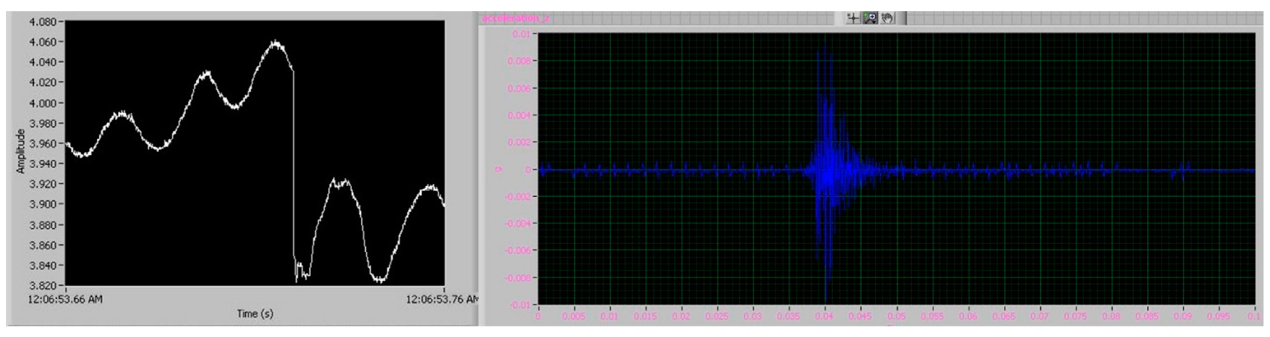
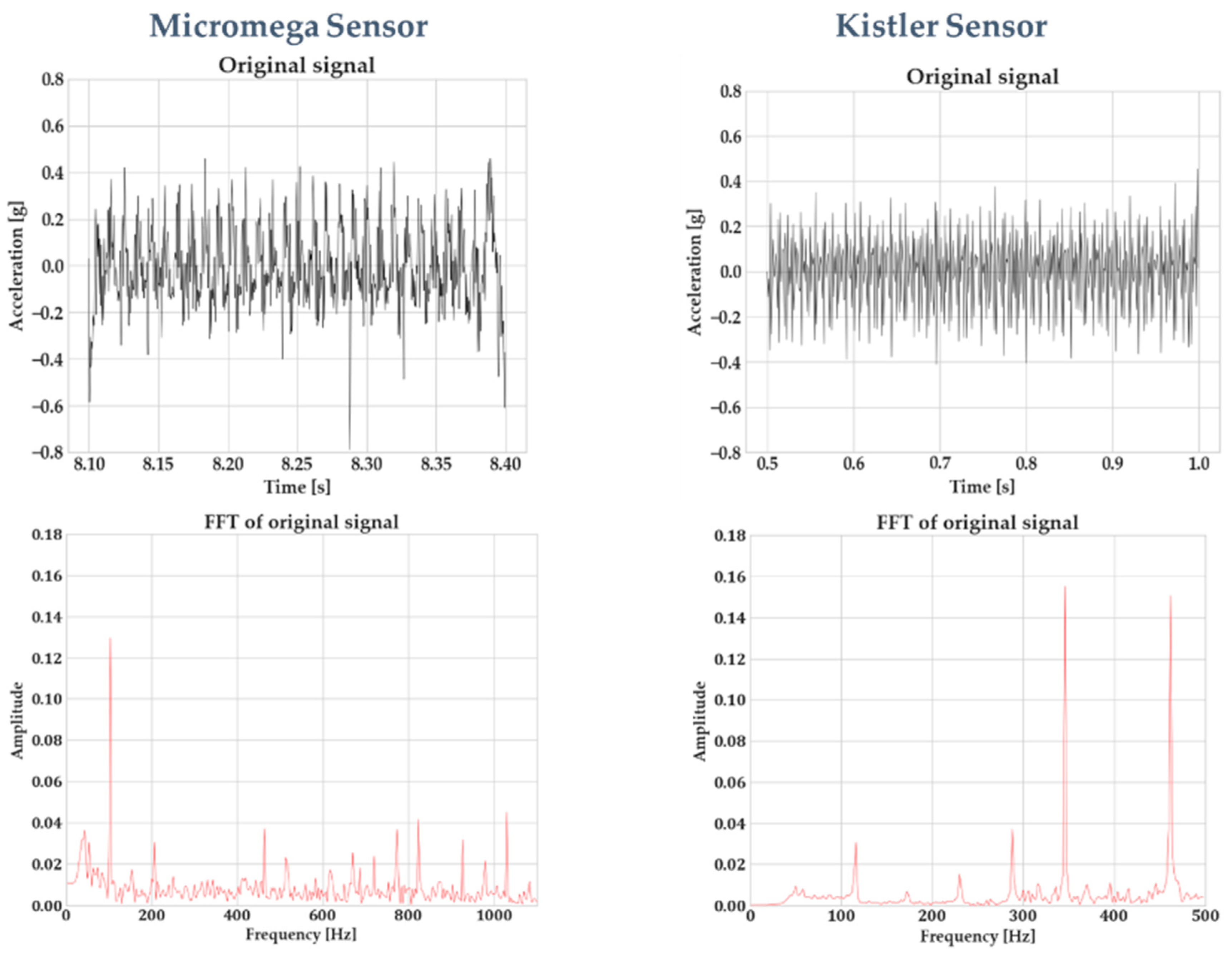
Figure 7 indicates this difference in data quality between the Micromega IAC-CM-U and the Kistler 8762A10 accelerometers. The signals were recorded with the sensors being integrated on the vice, using the same process parameters. It should be noted that the FFT spectrum for the Micromega sensor is larger due to the higher sampling rate that has been employed.
Figure 7 highlights this difference in signal quality. Two signals were generated by the Micromega and Kistler sensor, using the same process parameters (1 mm of axial depth of cut, 8 mm of radial engagement, 3100 RPM of spindle speed, and 0.18 mm feed per tooth). Window sampling was performed on the signals, and the window length was tailored for each sensor so that the frequency resolution of the FFT was the same. Due to the different sampling rates for each sensor (5 kHz for the Micromega and 1 kHz for the Kistler, with the second one being limited by the capabilities of the respective National Instruments DAQ), different window lengths need to be employed. Furthermore, the window length was minimized as much as possible because in a real-time chatter-detection application, the cycle time of the whole algorithm execution should be minimized as well. Nevertheless, the evidence of the inferior signal quality of the Micromega sensor is evident. Some numerical noise was introduced in the FFT of the Kistler sensor and was especially evident below 300 Hz due to the window length; however, the overall signal quality can be observed. Compared to the Micromega signal, on the other hand, the noise level at the whole frequency spectrum is evident. This is something for which the following steps of the algorithm compensate.
The use of advanced signal processing algorithms, together with artificial intelligence, has been greatly pursued within the last 5 years in order to detect chatter in milling from vibration signals [
6]. However, these algorithms are highly sensitive and prone to fault predictions when signal quality is impaired. In the next sections, we highlight how these algorithms are customized and optimized in order to increase their robustness, make them insensitive to poor signal quality, and continue exploiting their benefits for chatter detection.
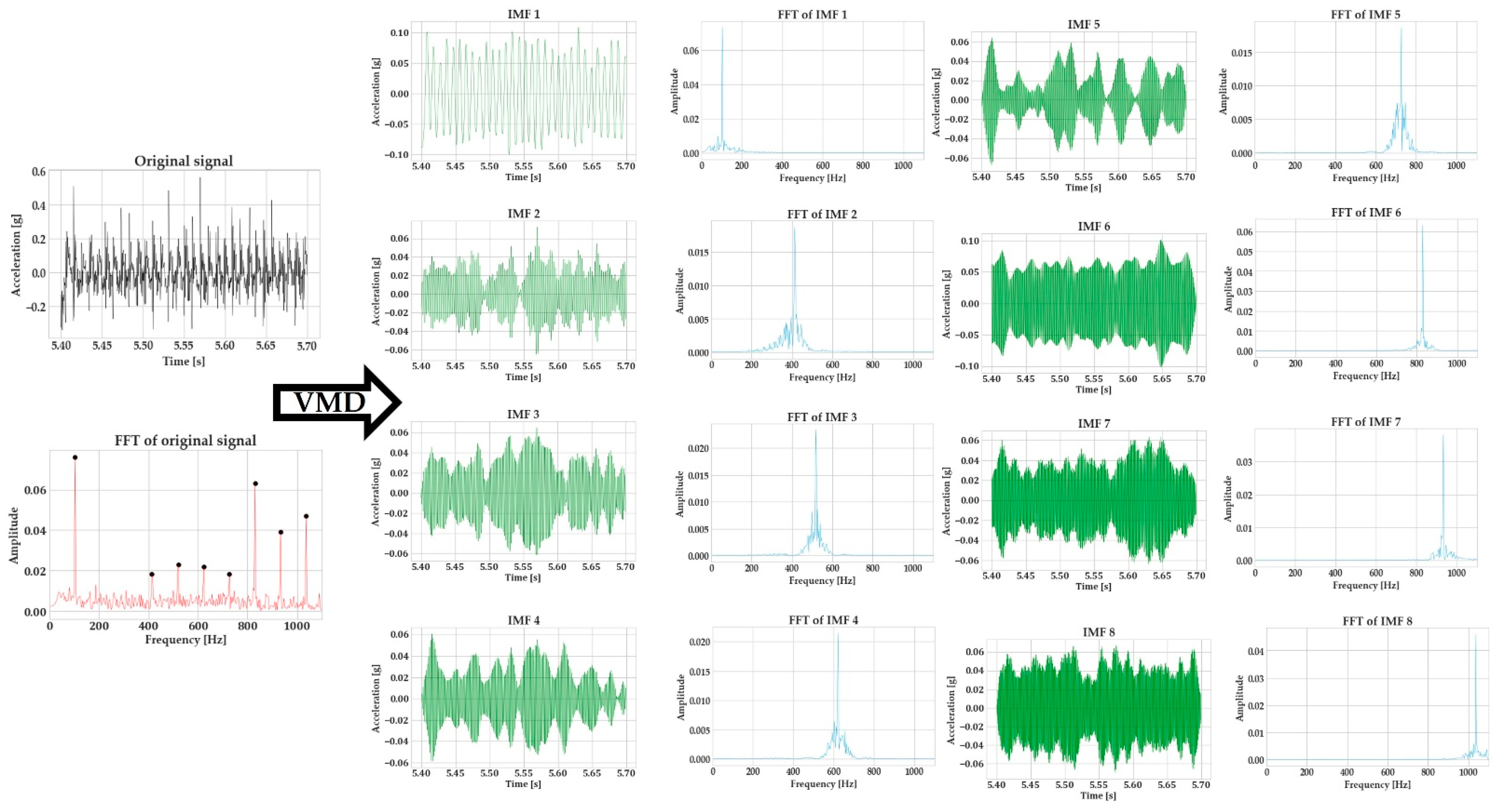
4.1. Vibration Signal Demodulation with Variational Mode Decomposition
Variational mode decomposition (VMD) is an algorithm for signal demodulation developed by Dragomiretskiy and Zosso [
27]. VMD is able to decompose a signal into its principal modes (
). These modes are amplitude-modulated–frequency-modulated signals, which are compacted around a center frequency and have specific sparsity properties. The prior sparsity of each mode is its bandwidth in the spectral domain. The superimposition of these modes can recreate the original signal. VMD is a popular algorithm for signal processing in medical applications [
28] and has found a use during the last years in the processing of signals generated by machining operations [
29,
30,
31].
In order to assess the bandwidth of each mode, VMD firstly computed the associated analytic signal through the Hilbert transform, with the aim of obtaining a unilateral frequency spectrum. The frequency spectrum of each mode is shifted by mixing it with an exponential tuned to the respective estimated center frequency. The bandwidth of each mode can be estimated through the H1 Gaussian smoothness of the demodulated signal.
Assuming an original time-series signal (
), its decomposition with VMD into a set of K modes becomes a constrained variational optimization problem, which can be formulated as follows:
where
and
are the modes and their center frequencies, respectively.
The constraint for accurate reconstruction of the signal through the superimposition of the modes is addressed by introducing the quadratic penalty term, also called alpha (
α), and the Lagrangian multipliers (
λ). The quadratic penalty term ensures reconstruction fidelity, especially when a noisy signal is processed, and the Lagrangian multipliers are a common way of enforcing constraints strictly. This process renders the constrained problem of Equation (1) into an unconstrained one, which can be formulated as follows:
This optimization problem is solved by the means of alternate direction method of multipliers (ADMM), leading to the following solutions for the modes (Equation (3)) and center frequencies (Equation (4)):
Considering that the vibration of the system of the milling process (cutting tool-workpiece–milling machine) can be safely assumed as multi-degree of freedom (DoF) oscillator, then by demodulating this vibration signal into several 1-DoF ones, it would be possible to identify the vibration mode that is related to chatter in a milling process. This makes VMD (and signal demodulation algorithms in general) ideal for chatter detection in milling. Nevertheless, their lack of robustness to signal quality (as explained below) is something that should be addressed to make them applicable for a wide range of sensors and a wide range of milling operations [
32].
VMD has two key hyperparameters that control the performance of the algorithm: the number of modes (K) that the signal should be decomposed into and the quadratic penalty term (α), which basically controls the bandwidth of each mode. The way that the poor selection of these two hyperparameters affects the decomposition quality is explained in detail in [
33]. In any case, it can be easily understood that selection of the wrong number of modes can lead to problems in signal decomposition. Specifically, these are mode mixing (when two modes are combined into a single one—a result of selecting a value for K that is lower than optimal, and the value of alpha allows the creation of wideband modes), loss of information (a mode is fully discarded—a result of selecting a value for K that is lower than optimal, and the value of alpha constrains the algorithm to create narrowband modes), and mode duplication (a single mode is decomposed into two—a result of selecting a value of K that is higher than optimal). It is evident how these three issues could impair chatter-detection performance in a system that is based on VMD for signal decomposition.
Additionally, it is important to have in mind that VMD is basically an optimization algorithm. As with all optimization algorithms, it suffers from the challenge of correct initialization. Specifically for VMD, the critical aspect is the correct initialization of the center frequency. The current available implementations of VMD offer three options of center frequency initialization: (i) all center frequencies are initialized at 0 Hz; (ii) the center frequencies are initialized uniformly, based on the bandwidth of the whole signal; and (iii) the center frequencies are initialized randomly. When the correct value of K is selected, the second initialization option usually produces good results. However, as the signal quality deteriorates, low-energy modes might be mixed with signal noise, leading to unpredictable results.
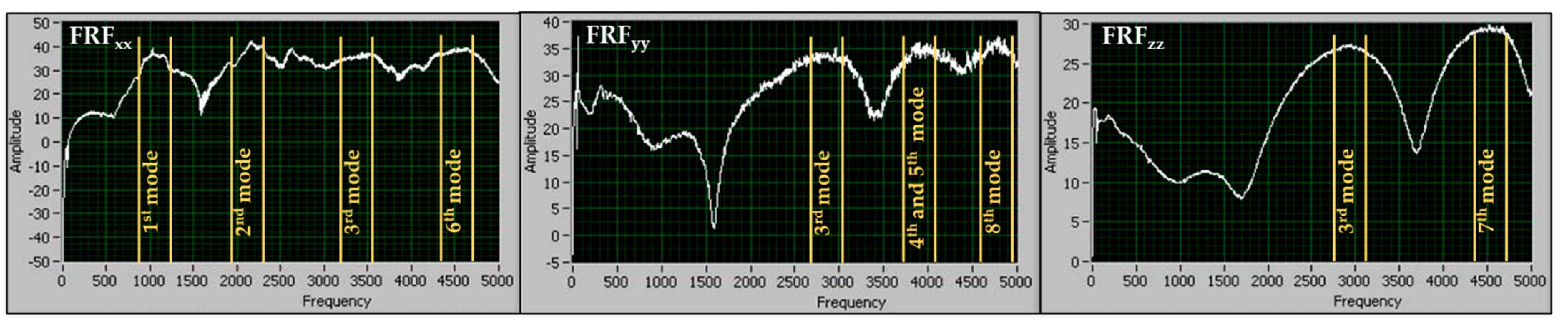
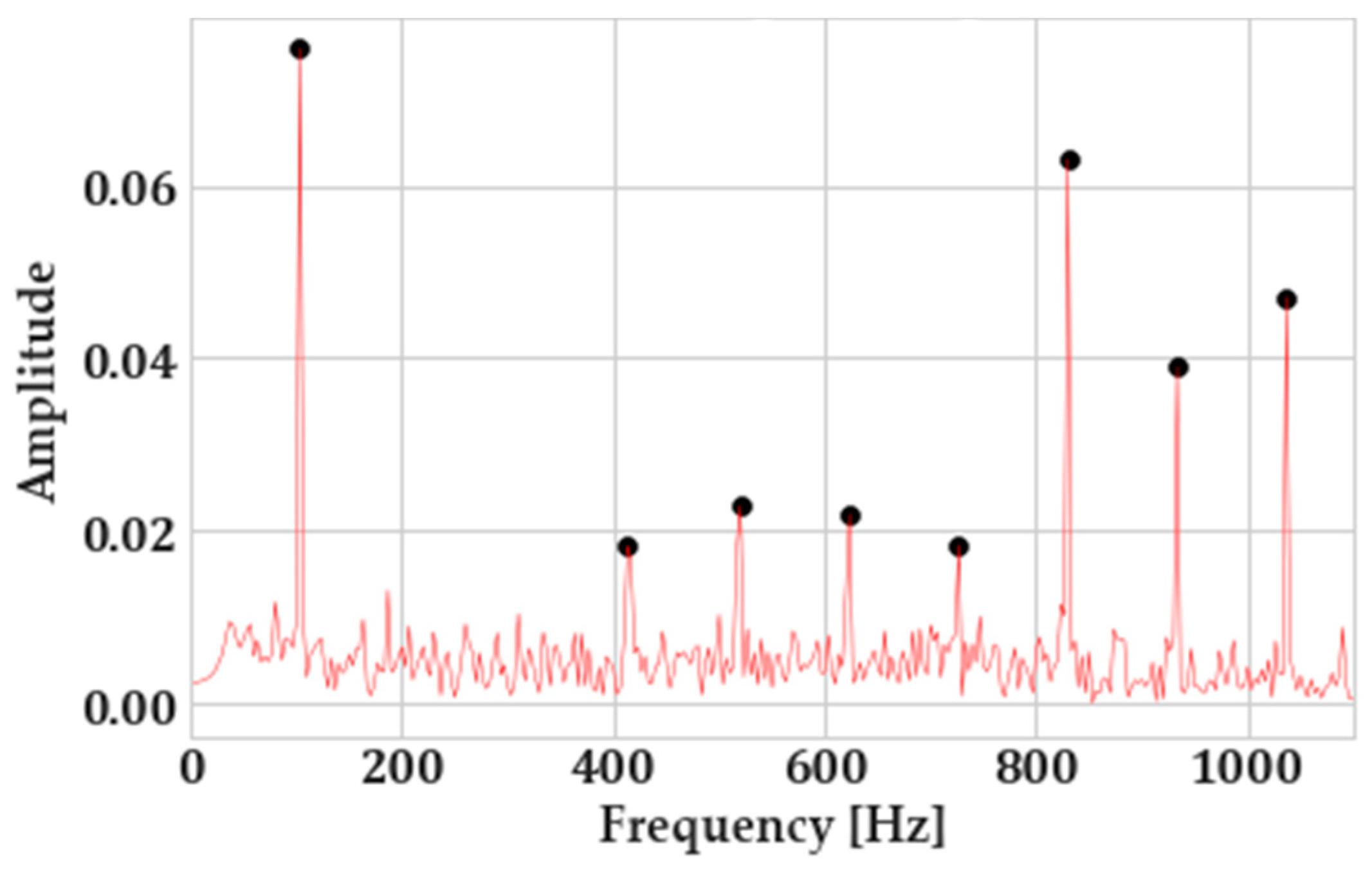
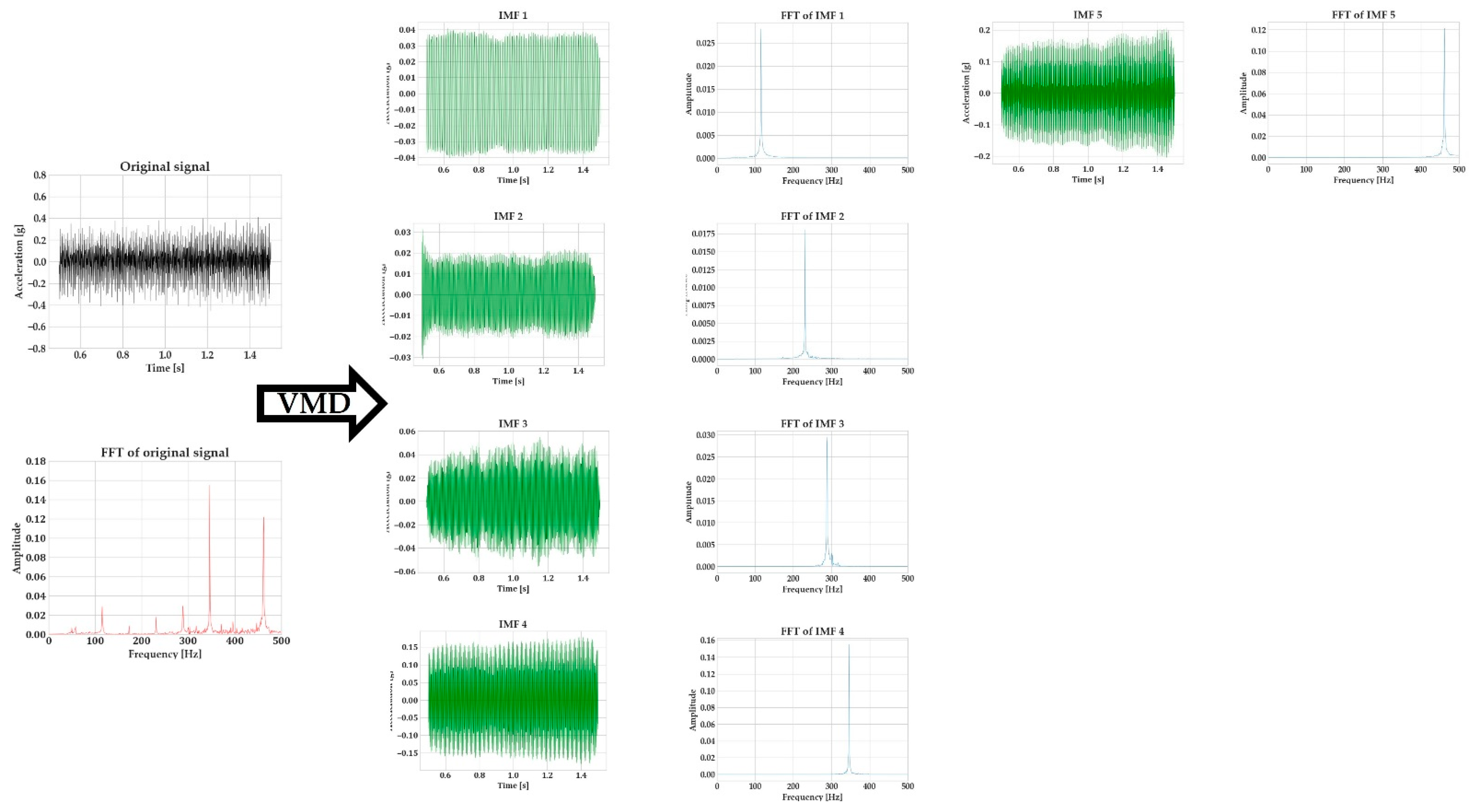
To tackle this and ensure correct initialization of center frequencies and thus the robustness of VMD to signal noise, peak picking is implemented in the fast Fourier-transform (FFT) of the vibration signals. For that, the “find_peaks” algorithm of SciPy (a highly popular package in Python for scientific computing) was utilized. The criterion that has been selected for the identification of a peak was its prominence, as it has been observed to be the most insensitive to the changes in the signal-to-noise ratio (SNR). The prominence of a peak explains how much it stands out due to its intrinsic height and its horizontal location with respect to other peaks.
Figure 8 showcases the way peak picking is utilized on the FFTs of the vibration signals.
This procedure ensures that both the number of modes as well as their center frequencies will be correctly identified and ensures correct decomposition. Additionally, it reduces the computational cost of the decomposition process since the algorithm does not need to iterate as many times, as in other initialization options. Finally, regarding the value of alpha (α), a relatively high value of 10,000 was selected through previous experience of the authors with the VMD algorithm [
32] to enforce the generation of narrowband modes.
4.2. Feature Engineering towards Chatter Detection
The study of the whole time-series signal or each mode separately (after decomposition) is a computationally heavy process, especially when high sampling rates (over 5kHz) are used in the monitoring system. As such, the extraction of features from the time and frequency domain that can indicate the presence of chatter and the evaluation of few numerical values instead of the whole signal increase the robustness of the system and reduce the cycle time of the chatter-detection operation.
Although the features that are extracted are statistical in nature, it was attempted to attribute a physical meaning to their selection. This entails the explanation of how a physical phenomenon that is exhibited during milling with chatter could be manifested in a statistical property of a time-series signal. This approach of performing feature engineering, considering the physics of the process ensures robustness of the generated features [
3], reduces the development and optimization time for the machine learning (ML) algorithm that will be used for chatter detection and facilitates the explainability of the ML predictions. The explainability is an especially important property for the whole system, as it facilitates the evaluation of its performance during the development phase as well as the interaction of its final user (usually a machine operator or process planner without significant experience in ML) during its use phase [
34].
The first feature that is calculated is the energy ratio between each individual mode and the whole signal. The energy of a discrete signal, sampled in the time domain, that consists of
n samples is formulated as follows:
Then, the energy ratio of the
k-th mode will be as follows:
where
E is the energy of the whole signal.
The energy ratio will work as a weighting factor for the calculation of all other signal features, and it is of high importance for the overall robustness of the approach. When stable milling takes place, the signal energy is gathered around the tooth-passing frequency and its harmonics. On the other hand, when the process starts to chatter, an energy shift from the tooth-passing frequency towards the chatter frequency takes place.
As a result, the energy ratio of each mode will capture this transition from harmonic frequencies to a chatter frequency. This supports the robustness of the approach against signal noise, signal disruptions, or other signal artefacts. Although statistically, they might exhibit some similar features with chatter, these signal artefacts will have a low energy contribution to the overall signal. In turn, their weighting with the energy ratio will suppress the features generated from signal artefacts and reduce the false positives (indication of chatter when the process is stable).
The next feature that is examined is the kurtosis of each mode. It is the fourth statistical moment of a signal, and it can describe how transient a signal is. The vibrations during stable machining are periodic and very low (even negative values) for the kurtosis can be expected. On the contrary, chatter (and especially its onset) is a transient phenomenon. As such, the kurtosis is expected to be higher when milling with chatter [
32]. The weighted kurtosis of each mode is calculated (using the energy ratio as a weight factor), and the maximum kurtosis of all modes is kept as a signal feature.
The next feature that is considered is the weighted autocorrelation. The cross-correlation of two discrete signals (α and ν) can be formulated as follows:
In Equation (7), the ¯¯ superscript denotes complex conjugation, while k is the value by which signal α is shifted in time with respect to signal ν, also called the lag value. If α and ν are the same signal, then it is possible compute the autocorrelation of this signal with its shifted self. Considering the lag value equal to the spindle rotation period, the autocorrelation of each mode is computed. A stable process is expected to have high autocorrelation (as the phenomenon is fully periodic), while chatter is expected to have low autocorrelation since transient phenomena take place. The weighted autocorrelation (using the energy ratio as a weight factor) of each mode is calculated and stored as a chatter-related metric.
Next, the weighted approximate entropy of each mode is calculated (using the energy ratio as a weight factor). In general, entropy-based algorithms are commonly used in information theory to identify the amount of irregularity in a signal as well as its information content. The approximate entropy can be used to determine the amount of irregularity and unpredictability of fluctuations of a time-series signal. A higher approximate entropy is expected when chatter takes place.
Finally, the spectral entropy of the overall signal is calculated and used as a feature. Spectral entropy is defined to be the Shannon entropy of the power spectral density (PSD) of the signal.
The features mentioned above are extracted from the x-axis and y-axis vibration signals, and a total of eight features is kept to be used as an input for the chatter-detection classifier.
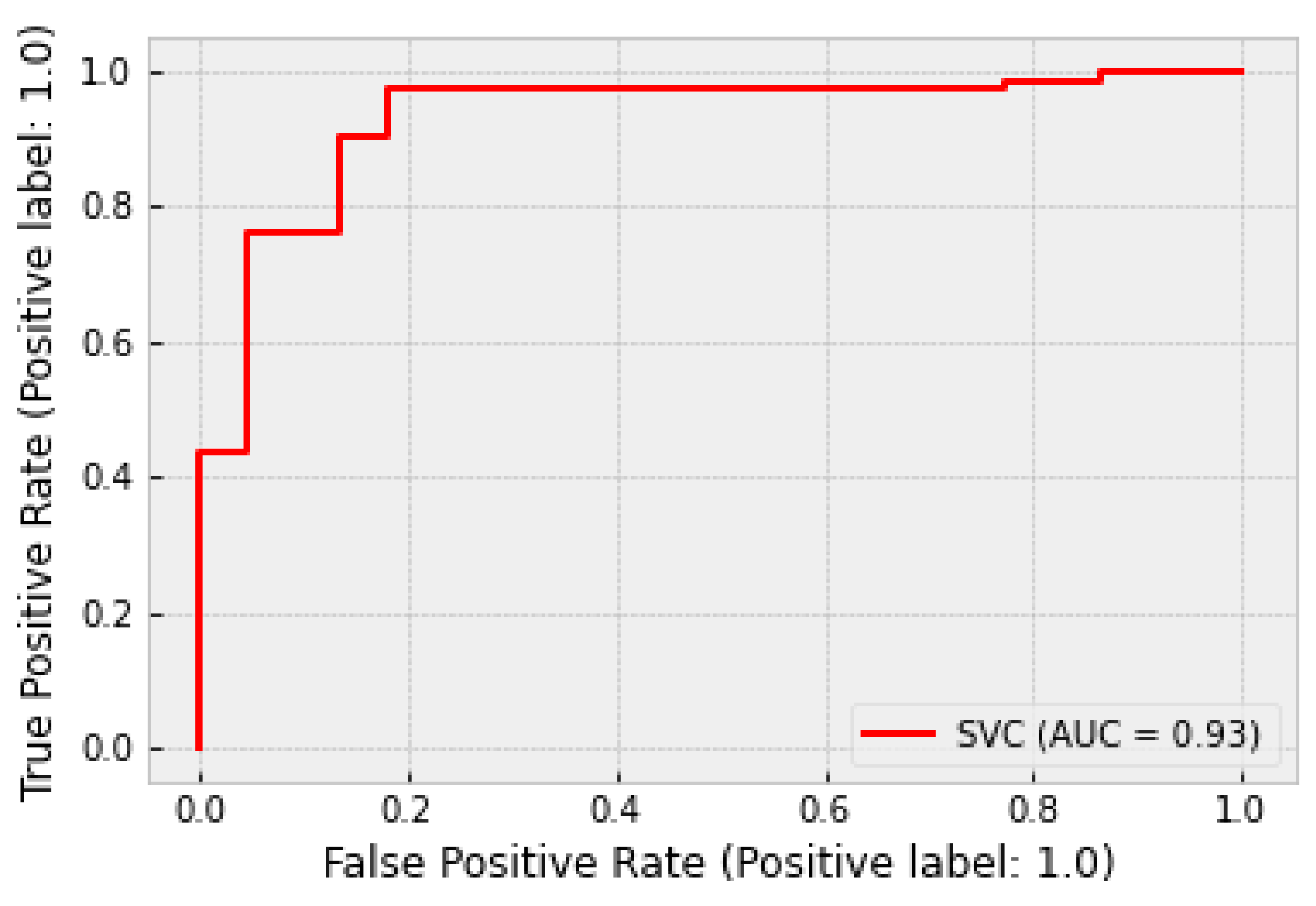
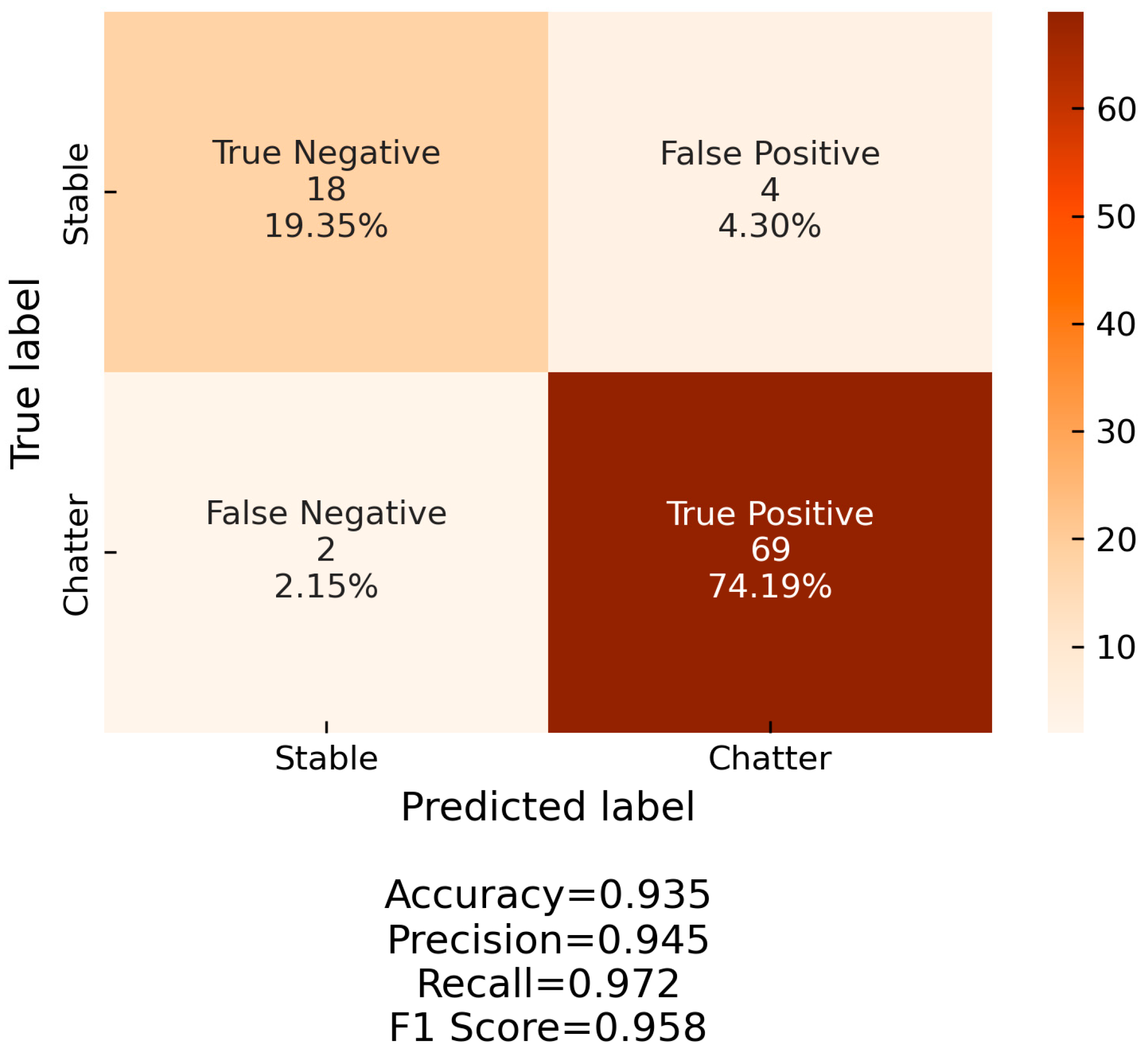
4.3. Chatter Detection
For the detection of chatter, a support vector machine (SVM) classifier was used. SVM is a very popular classification algorithm, which is characterized by a simple structure and training requirements while providing very fast classification speeds. The main goal of SVM is to construct a hyperplane that separates the training dataset with the maximum margin. The hyperplane has one less dimension than the dataset; in this specific case, the dimension of the dataset is the number of input features. For the tuning of SVM, three hyperparameters can be utilized: the kernel function, the magnitude of the slack variable (C), and the parameter gamma (γ). The kernel function is used to transform the dataset and explore the relationships between each data point in higher dimensions and is especially useful for handling non-linear datasets. The slack variable allows for misclassifications to occur during the training of the algorithm in favor of a larger margin between the hyperplane and the two datasets. The slack variable is used to tolerate outliers in the hyperplane construction. Finally, the parameter gamma determines the maximum distance a data point can have from the hyperplane in order to influence its construction.
For this specific application, a radial basis function (RBF) kernel function was selected. Additionally, an exhaustive grid search was performed to tune the C and γ hyperparameters. A 5-fold cross-validation scheme was employed, testing 1000 different values for each variable, evenly spaced in a logarithmic scale. The range for C was [0.01, 100000] and for γ the range was [0.00000001, 100]. Based on this optimization, the values of C = 1 and γ = 10 were selected. The SVM algorithm was implemented in Python using the scikit-learn package [
35].


 ,
, 
_Bikas.png)


