Abstract
This study focuses on modeling the yeast fermentation process using the hybrid modeling method. To improve the prediction accuracy of the model and reduce the model training time, this paper presents a semi−supervised hybrid modeling method based on an extreme learning machine for the yeast fermentation process. The hybrid model is composed of the mechanism model and the residual model. The residual model is built from the residuals between the real yeast fermentation process and the mechanism model. The residual model is used in parallel with the mechanism model. Considering that the residuals might be related to the inaccurate parameters or structure of the process, the mechanism model output is taken as unlabeled data, and the suitable inputs are selected based on Pearson’s maximum correlation and minimum redundancy criterion (RRPC). Meanwhile, an extreme learning machine is employed to improve the model’s training speed while maintaining the model’s prediction accuracy. Consequently, the proposal proved its efficacy through simulation.
1. Introduction
Yeast fermentation is one of the most important biomanufacturing processes as a new type of clean energy, and ethanol is an important substitute for fossil fuels. It is mainly produced by the yeast fermentation process. However, the growth of yeast is sensitive to environmental conditions such as temperature, PH, and substrate concentration. The yeast fermentation process involves a complex biochemical mechanism []. Therefore, it is difficult to build an accurate model of the yeast fermentation process.
Roles [] modeled the yeast fermentation bioreactor based on the kinetics of yeast growth. In addition to the kinetics of yeast fermentation, Nagy [] built a detailed model that involves heat transfer, the dependence of kinetic parameters on temperature, the mass transfer of oxygen, and the influence of temperature and ionic strength on the mass transfer coefficient. Considering the inhibitory effect of ethanol, a stripping model was proposed to further improve the prediction accuracy of the mechanism model []. Further, to recover ethanol from the gas mixture produced by the CO2 stripping method, Rodrigues et al. [] proposed an improved mechanism model based on the mass balance equation, stripping, absorption kinetics, and gas−liquid balance. Recently, a new modeling technique considered cell cycling, which can reduce yeast consumption and raw material costs []. Although the above mechanism model can well reflect the process flow and has good extrapolation characteristics, a large number of experiments may be needed to determine the kinetic structure, the parameters, and the mechanism of the yeast fermentation process, which all need to be fully understood.
For the data−driven method, detailed prior knowledge about the yeast fermentation process and mechanisms is not required. The process model is identified through a large amount of process data. Many data−driven methods based on machine learning have been widely used to develop fermentation process models. Ławryńczuk [] used a BP neural network to model and control the temperature of the bioreactor. Zhang [] employed a least squares support vector machine to establish a nonlinear model and to optimize the control of the process. Smuga−Kogut et al. [] took advantage of a modeling method based on the random forest to predict bioethanol concentration. Konishi [] estimated bioethanol production from volatile components in lignocellulosic biomass hydrolysates by deep learning. The extreme learning machine (ELM) proposed by Huang et al. [] greatly improved the computational speed because it only adjusted the weight of the output layer of the network and did not need to adjust the weight of the network through the gradient descent method like a BP neural network. The speed of learning is faster than a traditional support vector machine and neural network, and a similar generalization performance can be achieved. Sebayang et al. [] developed an ELM model to predict the performance of engines fueled by bioethanol. For data−driven modeling, the quality and quantity of the data are crucial to the quality of the model. For the yeast fermentation process, a large number of high−quality data points may be difficult to obtain due to the limitations of measurement techniques, long experimental cycles, etc. Useful data are essential to obtaining a satisfactory model that is based on data−centered modeling methods.
Hybrid modeling combines mechanism modeling with data−driven modeling, which not only considers the dynamics of a process but also reduces the demand for process data. In essence, hybrid modeling uses data to solve the mismatch problem of mechanism models and provides higher modeling accuracy. The structure of hybrid modeling is mainly divided into the serial [,,] and parallel structures [,]. For hybrid modeling with a parallel structure, the key is to build the residual model (RM), which utilizes the data−modeling method to model the residual between the mechanism model and process. The utility of the RM is to compensate for the mechanism model. At present, in the hybrid modeling framework, most studies use machine learning methods to train the RM, and the prediction accuracy of the nonlinear models obtained is higher than that of linear models []. Su et al. [] used a BP neural network to train the RM and verified the excellent prediction accuracy of the hybrid model combined with a BP neural network in the continuous polymerization processes. Niu et al. [] established a hybrid model using the least squares support vector machine to predict the substrate concentration and product concentration of a fed−batch fermentation reactor. Chen et al. [] applied support vector regression (SVR) and an artificial neural network to the hybrid modeling of continuous pharmaceutical processes. The hybrid modeling method effectively solved the model mismatch problem. The advantage of parallel structure hybrid modeling is that it can build an excellent model without considering the specific reasons leading to the mismatch of mechanism models and making new experiments. It only uses the RM to describe the dynamics that mechanism models cannot describe. However, the above studies are all supervised learning methods, which only consider the correlation between residuals and process inputs (control variables). Other factors related to residuals, such as oversimplification of the mechanism model and inaccurate model parameters, are not taken into consideration.
Semi−supervised learning refers to the fact that the learner combines labeled and unlabeled data to improve the learning performance []. In this paper, semi−supervised learning is considered to train RM, and the mechanism model output is taken as unlabeled data. However, filtering the data is necessary. Otherwise, the training burden of the model will be increased, and irrelevant data will even reduce the prediction accuracy of the model. Xu et al. [] proposed a semi−supervised feature selection method (RRPC) based on correlation and redundancy criteria for feature classification, which shows that the combination of labeled and unlabeled data improves feature selection. Considering the unconsidered dynamics, inaccurate model parameters, measurement uncertainty factors in the mechanism model, and model training speed, this paper adopts a parallel hybrid modeling method without considering the source of the mismatch in the mechanism model. The output of the mechanism model is taken as unlabeled data, the appropriate training data are selected through a RRPC algorithm for RM training, and then a set of nonlinear residual models are established by ELM. The established residual models are combined with the mechanism model to form a hybrid model. Finally, the effectiveness of the semi−supervised hybrid modeling method is verified by comparing its modeling accuracy and speed with those of the existing modeling methods.
2. Yeast Fermentation Bioreactor
The continuous yeast fermentation process for ethanol production is considered a simple continuous stirred reactor that involves continuously adding material to the bioreactor and removing the product from the reactor. Biomass (Saccharomyces cerevisiae) and the substrate (glucose) are the two main components of the bioreactor, and ethanol is the main product. The ideal operating conditions of the bioreactor are ingredients that are fully mixed, stirring speed, feed concentration, pH value, and a constant substrate feed flow and outlet flow from the reactor according to the requirements of the process.
The comprehensive model of the yeast fermentation process is as follows []:
where the input u of the model is the flow rate of the coolant and the output vector represents the biomass concentration, ethanol concentration, substrate (glucose) concentration, oxygen concentration, reactor temperature, and jacket temperature in the bioreactor, respectively. Fin, Csin, and Tin are the flow rate, concentration, and temperature of substrate feed, Fout is the outlet flow rate of the bioreactor, Tinj is the temperature of the coolant, is the oxygen saturation concentration, and V and Vj are the volumes of the bioreactor and jacket, respectively. Note: Fin = Fout; the total volume of reaction medium V remains constant.
In Equation (1), the maximum specified growth rate μx depends on Tr:
In Equation (4), the oxygen mass transfer coefficient is represented by the following temperature function:
the oxygen saturation concentration depends on Tr and pH (the overall effect of ionic strength):
The overall effect of ionic strength is as follows:
In Equations (4) and (5), the rate of oxygen consumption during biomass growth is:
for clarity, the parameter nomenclature and parameter values involved in models (1–11) can be found in reference [], respectively.
3. Semi−Supervised Hybrid Modeling Structure
The above model is the yeast fermentation process model. Although it can capture the main dynamics of the process, unconsidered dynamics, inaccurate model parameters, and measurement errors may lead to residuals between the mechanism model and the real process. The output vector of the actual process is defined as Yp, and the output vector of the mechanism model is defined as Ym; then the residual vector of the process is e = Yp − Ym, where . Before building RMs, we need to select the appropriate input data for each RM. The training data set is , including the input of the bioreactor and the output of the mechanism model. Each residual model requires different training data. The input vector is selected for the ith RM through RRPC as follows:
where φi represents the input selection function of the ith RM, i = 1, 2... 6, and e(i) represents the ith residual variable in the form of MATLAB code.
According to the selected input vector URMi and residual e(i), ELM is used to construct a group of RMs. The output of the ith RM is:
A group of RMs and mechanism models are combined into a hybrid model with a parallel structure, as shown in Figure 1. Yh = Ym + YRM represents the predicted value of the hybrid model, where is to compensate the mechanism model with the RMs.
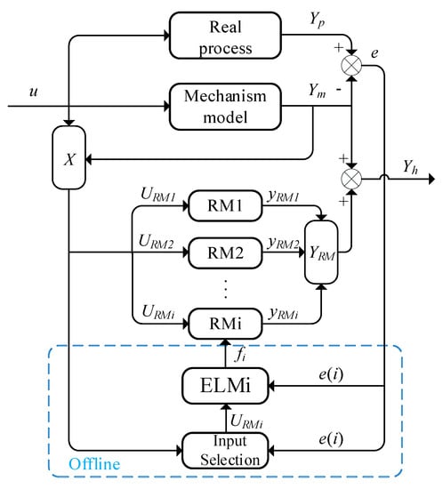
Figure 1.
The framework for semi−supervised hybrid modeling.
A residual model with good precision can be trained via supervised learning, but in the real process, the unconsidered model structure and incorrect parameters of a mechanism model may cause a deviation between the mechanism model and the real process. The purpose of this article is to let the output of the mechanism model be considered in the training data during the training of RM. The semi−supervised learning method based on RRPC is used to select appropriate inputs to establish RMs with better accuracy. Meanwhile, ELM is considered to train RMs to maintain good generalization performance and reduce the training time of the model. The semi−supervised hybrid modeling framework is shown in Figure 1, including the mechanism model, a group of RMs, an input selection module, and an ELM training module. The dashed box represents the offline training process of the ith RM.
4. Construction of a Residual Model (RM)
4.1. Input Selection for the RM
The output of the mechanism model was also used as the input of the training RM, and the maximum correlation and minimum redundancy criteria (RRPC) based on the Pearson correlation coefficient were used to select the best input and train the RM with the highest accuracy.
Pearson’s correlation coefficient is a method to evaluate the correlation between two vectors based on the covariance matrix of the data matrix. The residual vector is , and the input vector is . The Pearson correlation coefficient is used to describe the correlation between the jth input and the ith residual:
according to supervised input selection following the maximum correlation criterion, the input most relevant to the ith residual is obtained by . According to the minimum redundancy criterion for unsupervised input selection, the input with the least correlation with the lth input is obtained by .
The incremental search method is used to define the input vector selected by RRPC as URMi,k−1, in which there are k− 1 inputs, and then the kth input URMi(k) is selected from the remaining input vector {X−URMi,k−1}:
The input selection process of RM is shown in Algorithm 1:
| Algorithm 1. Select the ith RM input based on RRPC |
| 1: Input: residual vector e(i), input vector X, and number of target inputs s; |
| 2: Construct the target input set and available input set of the residual model; |
| 3: For k = 1 to s do; |
| 4: For each element Fj in U and each element Fl in URMi, select a new input according to Equation (16):
|
| 5: Update and |
| 6: End for; |
| 7: Output: URMi. |
4.2. RM Training
The input selection of the residual model is complete, and the residual model is trained by ELM. ELM is essentially a single hidden layer feed−forward neural network (SLFN), and its network structure is shown in Figure 2. The characteristic of ELM are that the parameters of the hidden layer are given randomly and the weights of the output layer are solved analytically, which can significantly improve the training speed of the model while maintaining the generalization performance similar to that of the traditional BP neural network. As the amount of data increases, applying ELM to train the residual model can save a lot of time.
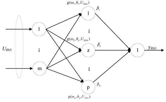
Figure 2.
Neural network structure of the ELM.
For the training of the ith residual model, given the training data {URMi, e(i)}, , and , m is the number of selected inputs and n is the data length, the output of the standard SLFN with P hidden nodes is:
where is the weight vector connecting the z hidden layer node to the input node, is the weight vector connecting the z hidden layer node to the output node, bz is the threshold of the z hidden node, is the activation function, and forms of the activation function are Sigmoid, Sine, Hardlim, and RBF, etc., and is the output vector of RM.
If SLFN with p hidden nodes approximates n training samples with zero error, i.e., , ωz, βz, and bz exist such that:
Equation (18) is expressed in matrix form as follows:
where H is the hidden layer output matrix of SLFN and the z column represents the output vector of the z hidden layer node associated with all inputs.
If the activation function is infinitely differentiable on any interval, the output weight matrix can be calculated by Equation (23) []:
According to Equation (24), the output of the ith RM is calculated as follows:
the ith RM construction process is shown in Algorithm 2.
| Algorithm 2. Construction of the ith RM |
| 1: Input: residual vector e(i) and input vector URMi corresponding to the residual vector; |
| 2: Divide input into the training and validation sets and perform data normalization; |
| 3. Initialize ω and b; |
| 4: H is calculated by Equation (20) according to ω, b, and the training set; |
| 5: Calculate β from Equation (21); |
| 6: The ith RM output is calculated by Equation (22) according to ω, b, validation set, H, and β; |
| 7: Reverse normalization; |
| 8: Output: YRMi. |
5. Modeling Method and Experimental Validation
5.1. Algorithm and Performance Index
According to the hybrid model structure and RM introduced above, the semi−supervised hybrid modeling process is summarized as follows:
- Collect the input u and output Yp of the yeast fermentation process, calculate the output Ym of the mechanism model, and calculate the residual e between the real process and mechanism model;
- Save u, Yp, Ym, and e in the database. Set time t = 1;
- Collect new data, calculate e according to step (3), and set t = t + 1;
- When t = n, select the appropriate input variables for each residual variable according to Algorithm 1;
- According to Algorithm 2, a group of RM is trained and used together with the mechanism model to form a hybrid model;
- Perform step (3) to calculate the output YRM of RM and the output Yh of the hybrid model.
Note: The final determination of the input variables of the residual model is measured by the prediction error. Two indexes commonly used to evaluate model accuracy in machine learning are the mean absolute error (MAE) and the root mean square error (RMSE).
The MAE is the average of absolute errors:
The RMSE is the square root of the mean square error between predicted and observed values:
where n is the data length, YRM(t) is the predicted value of RM at time t, and e(:,t)represents the real value of residual at time t in the form of MATLAB code.
5.2. Comparison between the Mechanism Model and the Real Yeast Fermentation Process
To evaluate the effectiveness of the proposed semi−supervised hybrid modeling approach, this section designs a simulation case based on an existing bioreactor model. Assuming that the models (1–11) are real process models, it is considered that the residuals are caused by incorrect dynamic structure, inaccurate modeling parameters, and sensor measurement errors during the process of mechanism modeling. Cell growth is affected by the concentration of dissolved oxygen, and biomass overgrows in the presence of excess dissolved oxygen, thus resulting in a decrease in ethanol production. Equation (11) describes the relationship between oxygen consumption rate and biomass growth. This paper assumes that the mechanism model describes the kinetic relationship between oxygen consumption rate and biomass growth as follows:
The biomass is the main factor affecting the ethanol production rate. The preexponential factor in the biomass growth rate model is related to the reaction collision cross section, number of molecules per unit volume, temperature, etc. It is assumed that the preexponential factor A1 in the biomass growth rate model in the mechanism model is not correctly identified, which is 2% lower than the real process. Considering that the acquisition of input and output signals is affected by sensor accuracy and measurement noise, the requirements for input and output signals are shown in Table 1 and Table 2 respectively.

Table 1.
Input signal requirements of the bioreactor.
Table 2.
Output signal requirements of the bioreactor.
The input is constrained between bounds, and the value is randomly chosen from a uniform distribution between the specified variation range value, which is consistent within 20 time steps, and each step is 1 h. The process runs for 2000 h. According to the above conditions, the outputs of the real process and mechanism model are shown in Figure 3, and there is a significant deviation between the real process and the mechanism model.
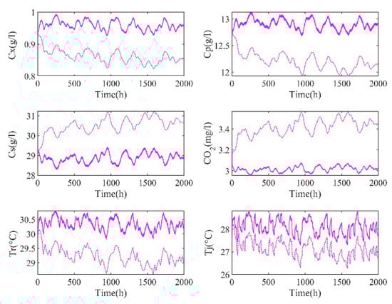
Figure 3.
Outputs of the real process and the mechanism model (the solid line is the real process, and the dashed line is the mechanism model).
5.3. Comparison between the Semi−Supervised Hybrid Model and the Mechanism Model
To evaluate the prediction effect of the semi−supervised hybrid model, the input should be selected by Algorithm 1 first, then the RM can be trained. RM trained with different inputs will produce different error values, which can be quantified by the MAE. To make the results more obvious, the ratio of the MAE with the semi−supervised learning method of the input selection module and that without the supervised learning method of the input selection module are used for demonstration, as shown in Figure 4.
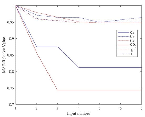
Figure 4.
The ratio of the MAE.
It can be seen from the figure that selecting an appropriate number of inputs can effectively improve the prediction accuracy of the model. Using too many useless inputs does not reduce the prediction error of the model but increases the complexity of the training. In addition, it can be seen from the figure that semi−supervised mixture modeling has the most obvious improvement effect on the biomass concentration and oxygen concentration predictions, which is also consistent with the model mismatch assumption above.
After input selection, the network should be trained by the ELM. The first 1800 time data is used as the training set, and the last 200 time data is used as the test set. Firstly, the parameters of the hidden layer are set to random values, and the sigmoid function is chosen as the activation function. Secondly, the number of hidden layer nodes was initialized, and then it was gradually increased on the basis of this value. Thirdly, we compared the predicted performance of the network. Finally, the number of nodes in the hidden layer was decided according to the best performance. Table 3 shows a set of training parameters and errors during the training of RMs. When the RMs are obtained, the RMs are used to predict the residual to compensate for the output of the mechanism model. Figure 5 shows the prediction errors of the mechanism model and the semi−supervised hybrid model. It can be seen that, compared with the mechanism model, the prediction error of the hybrid model is greatly reduced and close to 0.
Table 3.
Training parameters and prediction errors of the RMs.
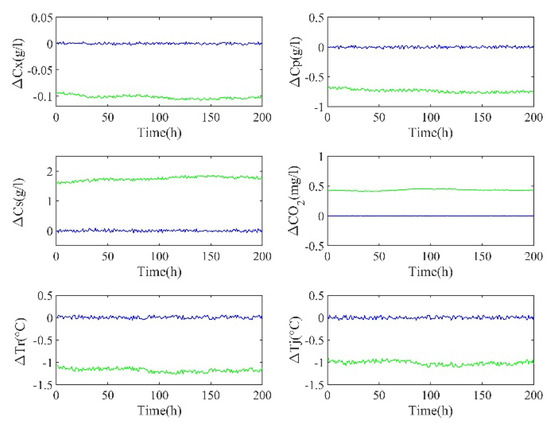
Figure 5.
Prediction errors of the mechanism model (green) and the hybrid model (blue).
5.4. Comparison between Semi−Supervised Hybrid Modeling and Ordinary Hybrid Modeling
In this paper, RRPC is used to select the inputs, and important process information can be extracted from the data to improve the accuracy of RM training. As shown in Figure 6, the absolute value of the prediction errors of semi−supervised hybrid modeling and ordinary hybrid modeling shows that the amplitude of ordinary hybrid modeling (red line) is higher, especially for biomass and oxygen concentrations. Meanwhile, to quantify the above results, Table 4 shows the MAE and RMSE of these two methods.
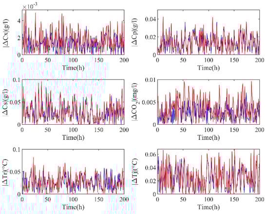
Figure 6.
Absolute values of prediction errors for semi−supervised (blue)/ordinary (red) hybrid modeling.
Table 4.
Prediction errors of semi−supervised/ordinary hybrid modeling.
5.5. ELM and the BP Neural Network
This section mainly compares the prediction accuracy and training time of the ELM and the BP neural network training RM. The two methods are simulated by MATLAB on a PC with a 3 GHz i5 CPU and 8 GB of RAM. The training data, number of hidden layer nodes, and activation function of the BP neural network are consistent with the ELM. Table 5 shows the comparison of accuracy and time between the two methods. It shows that the ELM has a similar generalization performance as the BP neural network, and the training time of the BP neural network is at least 10 times longer than the ELM. With the increasing quantity of data and complexity of network structure, the ELM can save a lot of training time, and ELM may be more suitable to be applied to online prediction.
Table 5.
Prediction accuracy and training time of the ELM and BP neural networks.
6. Conclusions
In this paper, for yeast fermentation process modeling, hybrid modeling with a parallel structure compensates the mechanism model by constructing a residual model, which not only avoids the optimization problem involved in the recalibration of the mechanism model but also reduces the number of experiments carried out by researchers and saves money and time. Compared to the existing supervised hybrid modeling, a semi−supervised hybrid modeling method based on an extreme learning machine is proposed, which not only uses a semi−supervised learning method to find useful data for residual model training to improve the prediction accuracy of the residual model but also improves the model training speed. Given the advantages of ELM, online hybrid modeling will be considered in future work. An additional issue that needs to be explored further includes building a framework to choose the corresponding hybrid model structure and network structure in different situations.
Author Contributions
Conceptualization, M.Z. and F.L.; methodology, M.Z. and F.L.; software, M.Z.; validation, M.Z. and F.L.; formal analysis, M.Z. and F.L.; investigation, M.Z. and F.L.; resources, M.Z., S.Z. and F.L.; data curation, M.Z.; writing—original draft preparation, M.Z.; writing—review and editing, S.Z. and F.L.; visualization, M.Z., S.Z. and F.L.; supervision S.Z. and F.L.; project administration F.L.; funding acquisition F.L. All authors have read and agreed to the published version of the manuscript.
Funding
This work was supported by the State Key Program of the National Natural Science Foundation of China (61833007).
Institutional Review Board Statement
Not applicable.
Informed Consent Statement
Not applicable.
Data Availability Statement
All data generated or analyzed during the study are included in the article, and the data that support the findings of this study are openly available.
Conflicts of Interest
The authors declare that they have no known competing financial interests or personal relationships that could have appeared to influence the work reported in this paper.
References
- Chen, J.; Zhang, B.; Luo, L.; Zhang, F.; Yi, Y.; Shan, Y.; Liu, B.; Zhou, Y.; Wang, X. A review on recycling techniques for bioethanol production from lignocellulosic biomass. Renew. Sustain. Energy Rev. 2021, 149, 111370. [Google Scholar] [CrossRef]
- Roels, J.A. Mathematical models and the design of biochemical reactors. J. Chem. Technol. Biotechnol. 1982, 32, 59–72. [Google Scholar] [CrossRef]
- Nagy, Z.K. Model based control of a yeast fermentation bioreactor using optimally designed artificial neural networks. Chem. Eng. J. 2007, 127, 95–109. [Google Scholar] [CrossRef]
- Rodrigues, K.C.S.; Sonego, J.L.S.; Cruz, A.J.G.; Bernardo, A.; Badino, A.C. Modeling and simulation of continuous extractive fermentation with CO2 stripping for bioethanol production. Chem. Eng. Res. Design. 2018, 132, 77–88. [Google Scholar] [CrossRef]
- Rodrigues, K.C.S.; Veloso, I.I.K.; Cruz, A.J.G.; Bernardo, A.; Badino, A.C. Ethanol recovery from stripping gas mixtures by gas absorption: Experimental and modeling. Energy Fuels 2018, 33, 369–378. [Google Scholar] [CrossRef]
- Ławryńczuk, M. Modelling and nonlinear predictive control of a yeast fermentation biochemical reactor using neural networks. Chem. Eng. J. 2008, 145, 290–307. [Google Scholar] [CrossRef]
- Zhang, H. Optimal control of a fed−batch yeast fermentation process based on least square support vector machine. Int. J. Eng. Syst. Model. Simul. 2008, 19, 63–68. [Google Scholar] [CrossRef]
- Smuga−Kogut, M.; Kogut, T.; Markiewicz, R.; Slowik, A. Use of machine learning methods for predicting amount of bioethanol obtained from lignocellulosic biomass with the use of ionic liquids for pretreatment. Energies 2021, 14, 243. [Google Scholar] [CrossRef]
- Konishi, M. Bioethanol production estimated from volatile compositions in hydrolysates of lignocellulosic biomass by deep learning. J. Biosci. Bioeng. 2020, 129, 723–729. [Google Scholar] [CrossRef] [PubMed]
- Huang, G.B.; Zhu, Q.Y.; Siew, C.K. Extreme learning machine: Theory and applications. Neurocomputing 2006, 70, 489–501. [Google Scholar] [CrossRef]
- Sebayang, A.H.; Masjuki, H.H.; Ong, H.C.; Dharma, S.; Silitonga, A.S.; Kusumo, F.; Milano, J. Prediction of engine performance and emissions with Manihot glaziovii bioethanol− Gasoline blended using extreme learning machine. Fuel 2017, 210, 914–921. [Google Scholar] [CrossRef]
- Psichogios, D.C.; Ungar, L.H. A hybrid neural network-first principles approach to process modeling. AIChE J. 1992, 38, 1499–1511. [Google Scholar] [CrossRef]
- Spigno, G.; Tronci, S. Development of hybrid models for a vapor−phase fungi bioreactor. Math. Probl. Eng. 2015, 2015, 801213. [Google Scholar] [CrossRef]
- Cabaneros Lopez, P.; Udugama, I.A.; Thomsen, S.T.; Roslander, C.; Junicke, H.; Iglesias, M.M.; Gernaey, K.V. Transforming data to information: A parallel hybrid model for real-time state estimation in lignocellulosic ethanol fermentation. Biotechnol. Bioeng. 2021, 118, 579–591. [Google Scholar] [CrossRef] [PubMed]
- Su, H.T.; Bhat, N.; Minderman, P.A.; McAvoy, T.J. Integrating Neural Networks with first Principles Models for Dynamic Modeling. In Dynamics and Control of Chemical Reactors, Distillation Columns and Batch Processes; Elsevier: Pergamon, Turkey, 1993; pp. 327–332. [Google Scholar]
- Ghosh, D.; Hermonat, E.; Mhaskar, P.; Snowling, S.; Goel, R. Hybrid modeling approach integrating first−principles models with subspace identification. Ind. Eng. Chem. Res. 2019, 58, 13533–13543. [Google Scholar] [CrossRef]
- Sansana, J.; Joswiak, M.N.; Castillo, I.; Wang, Z.; Rendall, R.; Chiang, L.H.; Reis, M.S. Recent trends on hybrid modeling for Industry 4.0. Comput. Chem. Eng. 2021, 151, 107365. [Google Scholar] [CrossRef]
- Niu, D.; Jia, M.; Wang, F.; He, D. Optimization of nosiheptide fed−batch fermentation process based on hybrid model. Ind. Eng. Chem. Res. 2013, 52, 3373–3380. [Google Scholar] [CrossRef]
- Chen, Y.; Ierapetritou, M. A framework of hybrid model development with identification of plant-model mismatch. AIChE J. 2020, 66, e16996. [Google Scholar] [CrossRef]
- Van Engelen, J.E.; Hoos, H.H. A survey on semi−supervised learning. Mach. Learn. 2020, 109, 373–440. [Google Scholar] [CrossRef]
- Xu, J.; Tang, B.; He, H.; Man, H. Semi−supervised feature selection based on relevance and redundancy criteria. IEEE Trans. Neural Netw. Learn. Syst. 2016, 28, 1974–1984. [Google Scholar] [CrossRef] [PubMed]
Disclaimer/Publisher’s Note: The statements, opinions and data contained in all publications are solely those of the individual author(s) and contributor(s) and not of MDPI and/or the editor(s). MDPI and/or the editor(s) disclaim responsibility for any injury to people or property resulting from any ideas, methods, instructions or products referred to in the content. |
© 2023 by the authors. Licensee MDPI, Basel, Switzerland. This article is an open access article distributed under the terms and conditions of the Creative Commons Attribution (CC BY) license (https://creativecommons.org/licenses/by/4.0/).