Minimizing the Effect of Specular Reflection on Object Detection and Pose Estimation of Bin Picking Systems Using Deep Learning

Abstract

The rapid evolution towards industrial automation has widened the usage of industrial applications, such as robot arm manipulation and bin picking. The performance of these applications relies on object detection and pose estimation through visual data. In fact, the clarity of those data significantly influences the accuracy of object detection and pose estimation. However, a majority of visual data corresponding to metal or glossy surfaces tend to have specular reflections that reduce the accuracy. Hence, this work aims to improve the performance of industrial bin-picking tasks by reducing the effects of specular reflections. This work proposes a deep learning (DL)-based neural network model named SpecToPoseNet to improve object detection and pose estimation accuracy by intelligently removing specular reflections. The proposed work implements a synthetic data generator to train and test the SpecToPoseNet. The conceptual breakthrough of this work is its ability to remove specular reflections from scenarios with multiple objects. With the use of the proposed method, we could reduce the fail rate of object detection to 7%, which is much less compared to specular images (27%), U-Net (20%), and the basic SpecToPoseNet model (11%). Thus, it is claimable that the performance improvements gained are positive influences of the proposed DL-based contexts such as bin-picking.

1. Introduction

Numerous industrial applications, such as object detection, robot arm manipulation, and bin picking, rely heavily on visual data gathered from cameras [1,2,3]. When light hits an object, two types of reflections occur, namely, diffuse reflection and specular reflection. As illustrated in Figure 1a, the former happens in objects with rougher surfaces, causing the light rays to disperse, enabling us to see the features of the object it reflected from. Specular reflection occurs primarily on smoother surfaces such as glossy or metallic material, in which the light rays directly reflect back. This causes a strong direct reflection, or a shining effect, named specular highlights. Figure 1b presents some examples of specular reflections. Although the human eye can clearly identify these simple objects, a computer program might identify them as more complex objects due to specular highlights and reflections [4]. Notably, the occurrence of specular reflection can also cause inaccurate feature identification, which degrades the consistency of comparing, matching, and consolidating objects through multiple images. As a result, typical computer vision applications, i.e., object detection and pose estimation, are significantly disrupted by specular reflection at the industrial level [5]. For example, the stereo-vision-based pose estimator designed by Wijenayake et al. [6] for bin picking relatively under-performs in cases of objects covered in glossy polythene wrappers compared with non-reflective objects.

In bin picking, cameras are used to obtain visual data from the objects of interest. These visual data are used to detect objects and their pose. Different model-based approaches and deep learning (DL)-based approaches were proposed to remove the effect of specular reflection, in order to enhance the accuracy of bin-picking.

In model-based approaches, some works incorporated a single image, whereas the others incorporated multiple images. Bajcsy et al. [7] proposed a single image model (SIM) approach that uses color information to separate reflection components. However, this approach is limited when two or more color transition regions of an image are washed-out due to the specular reflection. Another SIM-based approach was proposed by Tan et al. [8] using specular-free or specularity-invariant images. This approach was solid when the object’s surface had a complex texture. Similarly, Shena et al. [9] proposed a method for separating reflection components of uniformly colored surfaces based on the analysis of chromaticity and noise in the maximum chromaticity–intensity space. However, these approaches are not applicable if there are inter-reflections among surfaces and the specular reflection is slightly different from the color of the illumination.

Lee and Bajcsy [10] developed a multiple image model (MIM) based algorithm for the detection of specularities from Lambertian reflections using multiple color images from different viewing angles. Based on this algorithm, Lin et al. [11] proposed a method to separate specular reflections based on color analysis and multi-baseline stereo. Even though it achieved specular region reconstruction and true depth calculation of specular reflections, optimal performance was achieved only when certain constraints were satisfied. Kim et al. used a polarization filter in front of the sensor [12] and proposed a method that separates specular reflections from polarized color images based on line constraints in blue, green, and red (BGR) color space and spatial domain information. However, this work has a significant drawback as it cannot restore the variation of diffuse reflections with illumination color. Feris et al. [13] proposed a method that reduces specularity by solving a Poisson equation on a gradient field obtained from the input images. However, this method showed poor results in scenarios where the specular highlights do not shift among images to a significant degree.

Deep learning is a branch of artificial intelligence (AI) that seeks to imitate the functioning of the human brain and nervous system in order to enable machines to learn from their experiences and make decisions without explicit programming. It is an emerging field applied in many areas of engineering, especially for applications integrating vision technologies [14,15,16,17]. DL approaches were proposed for specular reflection removal also, and they were of two types: specific and general. Specific approaches can be applied for only specific scenarios or conditions. The method proposed by Funke et al. [18] is made explicitly for endoscopic images. Since this approach considers reflection variation caused by pulsation during the removal process, it is limited to removing specular highlights from endoscopic images. Shi et al. [19] proposed a work that extracts the material of an image and applies it to a 3D model in the ShapeNet dataset while controlling specular elements. However, the performance is considerably influenced by slower processing. Meka et al. [20] proposed the live intrinsic material estimation (LIME) model, which is primarily a material estimation model that is proven to separate specular and diffuse components successfully during extraction of materials from objects in an image. However, this network requires many components other than input and target images to train the model, which can be extremely complex and inflexible. Another work was proposed by Lin et al. [21] to directly remove specular reflections and highlights from images using a generative adversarial network (GAN), with a discriminator network involving multi-classes instead of binary classes. However, in this method, if stereo pairs of images are sent through the network one by one, the consistency of matching features across them is not guaranteed. The work proposed by Shihao Wu et al. [22] translates objects from specular to completely diffuse using multiple views. Although this approach incorporated feature consistency to a certain degree, this approach only considered input images that contained a single object that filled most of the image space.

We propose a unique solution for industrial use, where object detection and pose estimation must be carried out effectively on multiple small- to medium-sized reflective objects containing a high degree of specular highlights using only image data. The proposed system is named SpecToPose and consists of three main components: a dataset generator, a specular reflection remover, and a built-in object detector plus pose estimator (Figure 2). The implemented dataset generator satisfied the requirement for an ample dataset, which can be used for testing and training purposes. The specular reflection remover includes a DL-based specular reflection minimization algorithm and neural network model SpecToPoseNet. SpecToPose only considers improving stereo vision based pose estimation, which uses rectified stereo pairs of images. Furthermore, a unique object detector and a stereo-vision-based pose estimator were implemented to be used in a testing pipeline that evaluates each solution. All these components were finally packaged together to create a complete, user-friendly, flexible, and industrially usable system. The effectiveness of this solution was evaluated qualitatively and quantitatively. Rigorous evaluations were performed through a set of defined quantitative metrics and visual inspections. Consequently, the evaluations confirmed the superiority of SpecToPose with respect to existing DL-based approaches.

The rest of the article is organized as follows. Section 2 elaborately discusses the methodology of the proposed work. Performance evaluation is presented in Section 3. Section 4 presents the critical discussion, and conclusions are outlined in Section 5.

2. Materials and Methods

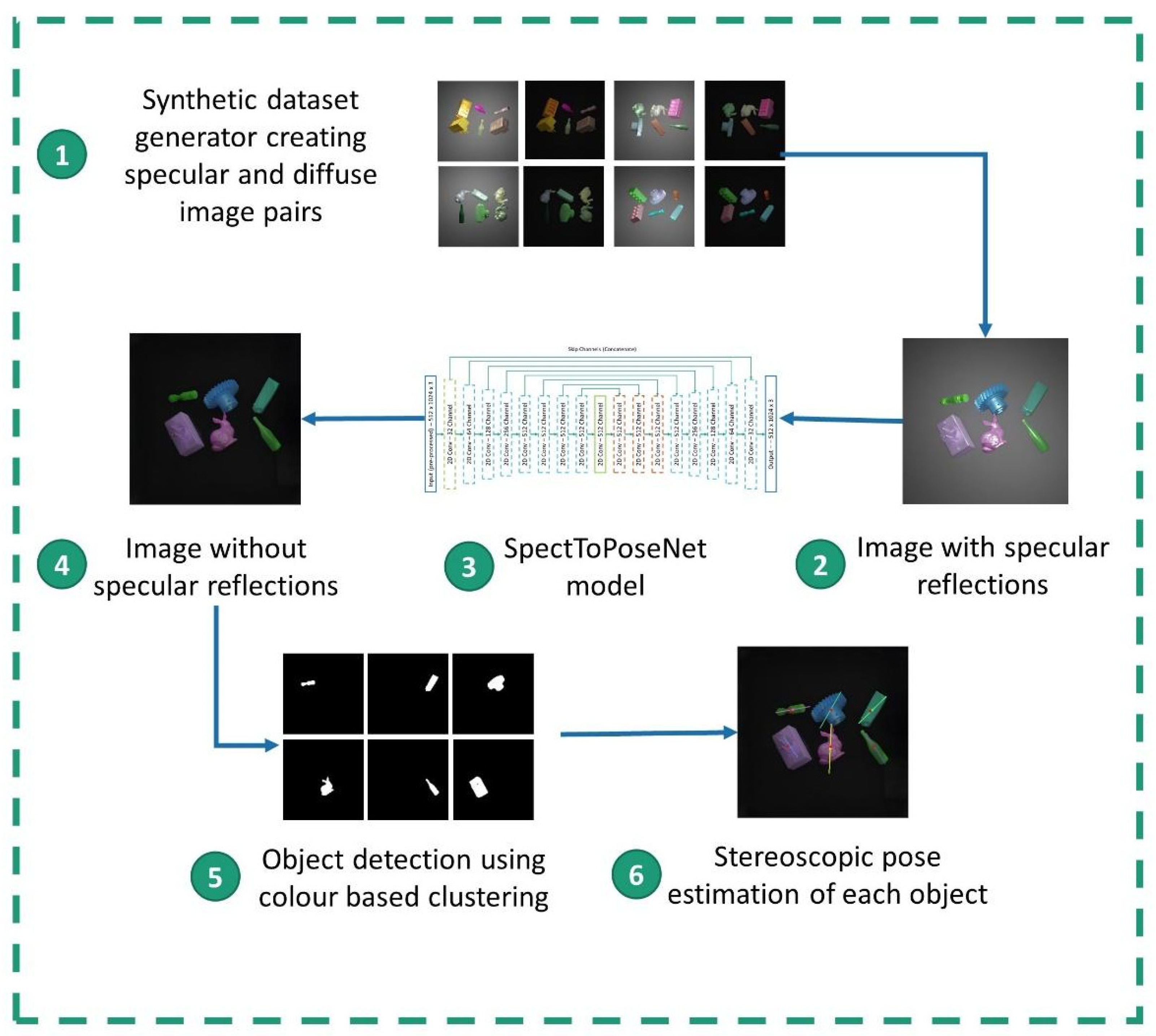
The first step of this research was to either gather or create a sufficiently large dataset that met the target use case of the project. Next, it was essential to implement a suitable testing pipeline to continuously test the results of each development iteration of the specular reflection remover. This pipeline consists of an object detector to separately identify each object in the scene and a stereo-vision-based pose estimator that can deduce the object’s location relative to the camera. Hence, the proposed SpecToPose system consists of three main components, namely, the dataset generator, specular reflection remover, and the combined object detector and pose estimator.

2.1. Dataset Generator

To develop and test the SpecToPose, a dataset is required that consists of images that conform to the specific target use case of this research. The images must contain a scene with multiple glossy or metallic objects of varying shapes and colors. The objects must be placed on a dark, flat surface, such as a bin. A strong enough light must also be directed at these objects to make them give out a significant amount of specular reflections. As this solution aims to improve stereo-vision-based pose estimation, images should also come in stereo pairs taken from two calibrated cameras. For the case of using a supervised deep learning approach, additional image pairs with no specular reflections are required for each image set described above to use as a target image for a network. The maximum variability of parameters such as object shapes, colors, light angles, and camera angles in the dataset is also preferred in order to build a highly generalized solution.

Finding a freely available image dataset that conforms to all of the above requirements is nearly impossible. Especially in the case of using DL-based methods, a significantly large dataset is essential to ensure satisfactory results that are not over-fitted. Due to this reason, a synthetic dataset generator was implemented in the SpecToPose system that can 3D render a sufficiently large dataset that meets all the requirements.

The open-source 3D graphics toolkit Blender was used to generate the required dataset [23]. Manually designing each and every scene in data points is not possible in the case of generating a large dataset. Therefore, the entire dataset generation process was automated using Python scripting that Blender supports. The generation script takes in a set of 3D models in Polygon File Format (PLY) files. There is an abundance of freely available 3D models of complex objects for this purpose, enabling the building of a dataset with various shapes and sizes.

Each randomly generated Blender scene would contain multiple objects (5 to 7), created by randomly selecting from the 3D model set, scattered across a dark plane. Overlapping of these objects is constrained as it is challenging to automate realistic overlapping of solid objects using Blender. The objects would be placed in randomized rotations and sizes (constrained to a limited range to ensure objects are not too large or small). Two light sources (point lights) are also placed above the objects in randomized locations around a circular perimeter so that the direction and placement of specular reflections can vary from scene to scene. The first camera is focused on the objects. The second camera is placed to only have a slight horizontal offset from the first camera (with no relative rotation, vertical or depth offset) so that the images are coplanar. This ensures that each pixel in two images has a horizontal epipolar line (no vertical variation), which ensures that no calibration or rectification has to be carried out when estimating the pose.

After rendering the stereo pairs of the scene with specular reflections, the exact same images without specular reflections are also required. To achieve this, the material of each object is changed into a matte finish (with low reflective properties). The light sources are also removed and replaced with a low-intensity area light (instead of a point light) to reduce the point reflective nature. A single data point in the generated dataset contains stereo pairs of images with and without specular reflections (four images in total) as shown in Figure 3, along with the location coordinates of each object in the scene relative to the first camera.

Additionally, the intrinsic properties of the cameras are saved as a calibration matrix $K$ (Equation (1)), where $f_x$ and $f_y$ are the products of the focal length and the pixel width and height, respectively; $u_0$ and $v_0$ are the coordinates of the principles point of the image; and $\gamma$ is the skew coefficient (set to 0). The extrinsic parameters for each camera in respective to the Blender world coordinates are also saved in the form of a $RT$ matrix, as shown in Equation (2), where $R_{3\times 3}$ refers to its rotation matrix and $T_{3\times 1}$ refers to its translation matrix. Using this setup, a dataset of 1500 data points was created, which is sufficient enough to be used in a deep learning application.

$$K=\left[\begin{array}{cccc}{f}_x& \gamma & u_0& 0\\ 0& f_y& v_0& 0\\ 0& 0& 1& 0\end{array}\right]$$

(1)

$$RT={\left[\begin{array}{cc}{R}_{3\times 3}& T_{3\times 1}\\ 0_{1\times 3}& 1\end{array}\right]}_{4\times 4}$$

(2)

2.2. Object Detection

The ultimate objective of the SpecToPose system should be to use it on images with any object without limiting it to a particular predefined object. However, a completely general object detection algorithm that can be used in such a situation has not surfaced so far. There are some popular algorithms such as R-CNN [24], Fast R-CNN [25], Faster R-CNN [26], and YOLO [27], and pre-trained convolutional neural networks that are widely used for object detection applications such as AlexNet [28], VGGNet [29], and ResNet [30]. These networks will only work on generic objects but will not work for specific objects. Even when tested on a dataset generated using 3D models of generic objects, such as cars, spoons, or bottles, the accuracy levels were very low. Hence, through the combination of some existing technologies, a simple approach was implemented for object detection and segmentation with certain constraints.

The algorithm explained below requires single-color objects in the image and works best if the objects in the scene are spread out with little overlapping. If the overlapping is between objects of different colors, the algorithm can distinguish them. However, if the color is the same, it may detect them as one single object. The first step of this approach was to convert the images from the BGR color space to the hue, saturation, and value (HSV) color space. In the BGR space, the components are correlated with the image luminance and with each other, making discrimination of colors difficult [31]. By converting into the HSV space, image luminance is separated from the color information, making the objects pop out better from the background and each other, as shown in Figure 4.

The next step is to segment the image using the color information [32], and K-means clustering was chosen for this purpose. First, the HSV image is clustered with a relatively high number of clusters to separately identify segments of the image based on the color. The HSV image is then converted back to the BGR space and clustered again using the same K-means algorithms but with a lower cluster number (Figure 4c–e). The reason for the second clustering is to ensure that the single object is not detected as two separate objects, which can be clearly seen in Figure 5a.

The pixels in the image are then split into separate images based on their cluster. For an example, if the image contains two clusters only, the image is split into two images, each containing only the pixels related to that cluster. The next step is to take each of these images and find the connected components to separately identify the objects, as seen in Figure 6. A connected component algorithm such as Tarjan’s algorithm [33] with 8-connectivity can be used for this with few filters to remove too large or too small regions. These connected components are then used to create a set of masks, which can later be used to separate the object from the rest of the image.

2.3. Pose Estimation

The final element of SpecToPose is to estimate the pose of the objects detected in the previous step. Two rectified images can be used to find the horizontal and vertical location of a point with respect to camera coordinates by backwards projection using the projection matrix. To calculate the depth, the disparity-to-depth-map matrix $Q$ in Equation (3) is calculated, where $c_x$ and $c_y$ are the principal point in the left camera, $c_x^{\prime }$ is the horizontal coordinate of the principal point of the right camera, $f$ refers to the focal length of the cameras, and $T_x$ is the horizontal translation between the two cameras. These parameters can be derived using the calibration matrix $K$ and extrinsic matrix $RT$ of the cameras.

$$Q=\left[\begin{array}{cccc}1& 0& 0& -c_x\\ 0& 1& 0& -c_y\\ 0& 0& 0& f\\ 0& 0& -\frac{1}{T_x}& \frac{c_x-c_x\prime }{T_x}\end{array}\right]$$

(3)

Next, the disparity map is generated for the stereo image pair areas as shown in Figure 7 using a modified version of the semi-global matching (SGM) algorithm [34]. Then, the pixels in the image are filtered out, where the disparity cannot be calculated correctly using some threshold values. Furthermore, the segmentation masks obtained through object detection are used to filter out unwanted pixels. Using the $Q$ matrix and the disparity map, the location coordinate of every pixel is obtained with Equations (4) and (5). The values $u$ and $v$ refer to coordinates of the pixel on the left image and $d$ is the disparity at that point. Finally, $x$, $y$, and $z$, corresponding to horizontal, vertical and depth coordinate of the point, are calculated with respect to the left camera in world coordinates.

$$\left[\begin{array}{cccc}1& 0& 0& -c_x\\ 0& 1& 0& -c_y\\ 0& 0& 0& f\\ 0& 0& -\frac{1}{T_x}& \frac{c_x-{c_x}^{\prime }}{T_x}\end{array}\right]\left[\begin{array}{c}u\\ v\\ d\\ 1\end{array}\right]=\left[\begin{array}{c}u-c_x\\ v-c_y\\ f\frac{c_x-{c_x}^{\prime }-d}{T_x}\end{array}\right]=\left[\begin{array}{c}X\\ Y\\ Z\\ W\end{array}\right]$$

(4)

$$x=\frac{X}{W}, y=\frac{Y}{W}, z=\frac{Z}{W}$$

(5)

In order to estimate the translation of the objects from the camera, the centroid in world coordinates is calculated and taken as the coordinates of the center of the object. For arbitrary objects, there is no way to correctly define the rotation of the object as the orientation in the $\left(0,0,0\right)$ position is unknown. As an approximation, this pose estimator will iterate through the real-world location of all points corresponding to the object and find the point that is the furthest from the above-calculated center, and take the line joining them as a rotating axis of the object, as shown in Figure 8a. The red dots of Figure 8b correspond to the actual center point of the object (saved during the dataset generation) and the colored dot is the estimated center.

2.4. Preprocessing for Deep Learning

When exploring deep learning approaches, the large synthetic dataset generated comes in handy. In each data point, the image with the specular reflections can be called the specular input to the network. The diffuse counterpart of it can be called the target diffuse, meaning the ideally perfect output to expect from the network. The network output can be compared with the target diffuse to form an error function to train the network, such that the output can become more and more similar to the target.

It is always better to reduce the glare effects as much as possible from the input using image processing techniques before feeding them to a neural network. The contrast limited adaptive histogram equalization (CLAHE) is an excellent method to bring down high contrast areas of the image (glares) [35]. This algorithm works better in the HSV color space; therefore, both the specular input and diffuse target are converted to it. The CLAHE algorithm can be directly applied to the value channel of the specular input image and clipped using a constant value (set through trial and error). Inpainting is another technique that can be used to further reduce the glares in the image by coloring the glare points based on the neighboring pixels. First, a copy of the image is taken and converted to a gray scale, and a Gaussian blur is applied. Then, it is thresholded with a high value to find the points of the image that contain the specular highlights and they are used as a mask when applying the Telea inpainting algorithm [36]. Figure 9a shows an example input, while Figure 9b and c depict the results of histogram equalization and the inpainting, respectively.

The pixel values of an image are in the range of [0, 255], making it unsuitable for use in a neural network. The neural network needs inputs and targets within a fixed range of data that can be ensured through some activation. All the values in the image are normalized to the range of [−1, 1], so that the output layer of the network can apply a $tanh$ activation to ensure an output in the same value range. During inference, the network output values have to be brought back to the original [0, 255] range to construct a meaningful image.

2.5. Initial Neural Network Architectures

A convolutional neural network (CNN)-based approach is the best approach to tackle problems of visual imagery. The network should take an image as an input and provide another image as the output after transforming it. The basic starting point to develop such a network is, to begin with, a simple convolutional auto encoder (CAE) [37]. The CAE contains two main parts, namely, the encoder and the decoder. The encoder would take the image as an input, and through convolutional layers, the spatial dimensions would be reduced, while increasing the number of channels. The final layer is then flattened and further reduced to create a middle layer called the embedded layer. The decoder’s job is to take the embedded layer and increase the dimensions through convolutions to produce an output with the same shape as the input. The network is trained by comparing the mean squared error between the output and target.

Figure 10 depicts the basic architecture of the CAE. It has fewer layers than the actual implementation for simplicity. The output of the target is compared with the target diffuse to train and the results of an example can be seen in Figure 11. It is clear that a simple CAE network is not suitable for images containing complex details. A large amount of details are lost in the output, and there is some unnecessary noise in the output. Hence, the next step is to modify the network to keep some of the features of the input image intact during the transformation process. A flattened embedded layer in the middle can also contribute to this issue, as a significant amount of spatial data can be lost by it; hence, avoiding it altogether is another option. There is also the possibility of a vanishing gradient through the network in the latter stages of training, requiring a small learning rate.

The U-net architecture [38] has come into popularity recently for image to image translation, and it addresses the problems faced in the above network. It has an encoder–decoder-style architecture with contracting and expansion layers at its core. The two sides are symmetrical, which gives it the signature U shape. This architecture removes the fully connected layers altogether. One special feature of this architecture is the inclusion of skip connections from the encoder layers to the decoder layers with the same dimensions, which concatenate them together. These skip connections serve two purposes; first, they pass features from the encoder layers to the decoder layer so that they can recover some spatial information lost during the contraction; second, they provide an uninterrupted gradient flow, tackling the vanishing gradient problem.

As shown in Figure 12, a slightly modified version of the original architecture was implemented, which contains sets of convolutional layers with an increasing number of filters, along with ReLU activation across them. Max pooling is used to contract the spatial dimensions of the layers in the first half of the network. In the latter half, the spatial dimensions are recovered through up-sampling, and the corresponding layer output with the exact dimensions in the first half is concatenated to it. Following this approach yielded better results compared to the previous iterations.

As this system works in stereo pairs of images, going through the network twice is required during generation time. This can double the inference time, making the entire operation much slower. Instead of inputting a single camera view image at a time, combining the left and right image together to make a single input and feeding it to the network to obtain the left and right image output together is a feasible approach. One option is to concatenate the images channel-wise, and the other is to concatenate them spatially. Shihao Wu et al. [22] found that concatenating the pairs horizontally led to the best results. This approach is much simpler to perform and allows more straightforward error calculation and output extraction. As the stereo pairs are rectified, this approach also establishes a connection between pixels on the same horizontal lines and helps to maintain matching points during the translation.

2.6. SpecToPoseNet Architecture

So far, the convolutional neural networks that were implemented rely solely on the mean squared error between the output and the target. Even though this error is reduced while training, it does not guarantee the authenticity of the output. Hence, the output still does not look realistic enough compared with the input and output. GAN [18] is a popular development in the world of neural networks that boasts of providing extremely realistic and authentic-looking outputs. It is commonly used for generative or translation work, perfectly matching our use case. GAN is also used in works such as Shihao Wu et al. [22] and John Lin et al. [21] to minimize reflective effects. Over-fitting is common in very large networks and standard encoder–decoder-style networks. GAN incorporates randomness in the middle of traditional generators in GAN by sampling from a latent space instead of directly taking the layer output. The other portion of the GAN architecture is the discriminator network. The input for this network is a concatenation of the specular input and the diffuse target or the specular input with the generator network’s output. The input can be named the ideal input for the former, while the latter can be called the translated input. The discriminator network is trained to properly distinguish these two inputs and provide a label to them. Therefore, when the ideal input is given, the network should output a label of all ones, and when a translated input is given, it should give a label of all zeros in a perfect scenario. Similar to the encoder portion of the generator network, the concatenated input’s spatial dimensions are reduced through convolutions while increasing the channel size, as seen in Figure 13. The layers similarly use Leaky ReLU activations along with batch normalization (except in the first layer). The final layer is subjected to a convolution with a single filter, resulting in a single channel output. A sigmoid activation is applied here such that the output values are in the [0, 1] range expected from the discriminator label. As with the generator network, this was also implemented so that it is auto-scaled to fit the input image’s dimensions. The proposed deep learning model is named the SpecToPoseNet, and it is developed based on the Pix2pix [39] GAN architecture, which specializes in the image to image translation using conditional adversarial networks.

The U-Net model that was implemented in the previous iteration can be modified and taken as the generator network shown in Figure 14. The encoder of the network consists of 2D convolution layers with a stride of two, such that the spatial dimensions are halved in each layer. The input image has three channels, which are increased to 32 by the first convolutional layer and subsequently increased until the middle layer is reached. The decoder layers then use 2D transposed convolutional layers to contract the channels by 2 in each layer until reaching 32 and finally giving a three-channel image output. The spatial dimensions work the opposite way, with encoders reducing them by 2 in each layer; a vertical dimension of 1 is reached and again increased to the original image’s dimensions. Due to the usage of strides of 2 throughout the network, the input image’s horizontal $y$ and vertical $x$ dimensions must be of a power of 2, and the condition $2\times y\le x$ must be satisfied.

Batch normalization is also used in almost all the layers in the generator, which can help stabilize and accelerate the learning process [39]. As seen in Figure 14, the first layer does not use batch normalization as by doing so, the colors of the input image can become normalized based on the batch and be ignored. Since the color should be preserved intact, especially for the implemented object detection algorithm, batch normalization is omitted in the first layer. ReLU activation is used in all layers to avoid the vanishing gradient problem that other activation types suffer. Simple ReLU activations, which provide a better sparsity in the layer outputs (act more closely to real neurons), are used in the decoder layers, while Leaky ReLU activations that avoid the dying ReLU problem are implemented in the deeper encoder layers. Only in the final layer, a $tanh$ activation is used to bring the output to the desired range.

SpecToPoseNet requires to be highly generalized, especially as the solution at hand is expected to work in any case if trained correctly. Avoiding over-fitting of the network is highly important for this purpose. Instead of using real data, a synthetic dataset was generated, nevertheless the network is also expected to work on real data. When training with the dataset, it can easily be overfitted to the synthetic data, providing inferior results in real-world scenarios. For this generator, as proposed in the Pix2pix architecture, dropout layers are incorporated into the network’s decoder potion to add a source of randomness to it. These layers are responsible for randomly dropping nodes during training and generation, which helps to avoid the over-fitting problem [40].

2.7. Training the Networks

When training the SpecToPoseNet, multiple types of losses are calculated and combined. The loss relating to the discriminator network is the adversarial loss. The discriminator network is a classification network responsible for assigning class 0 across the output for a translated input and class 1 for an ideal input. Binary cross-entry entropy loss is a trendy way to evaluate such networks, and it can be calculated using Equation (6), where $N$ is the points in the output, $y_i$ is the label, and $p\left(y_i\right)$ is the probability output of the node.

$$los{s}_{ad}=-\frac{1}{N}{\displaystyle \sum }_{i=1}^N{y}_i\cdot \log \left(p\left(y_i\right)\right)+\left(1-y_i\right)\cdot \log \left(1-p\left(y_i\right)\right)$$

(6)

In the case of the generator, multiple loss components are calculated, weighed, and used during back-propagation. One of the significant losses is the same adversarial loss explained above, applied to the generator training as well by sending the generator output through the discriminator network. However, in this case, the difference is that the loss is calculated by comparing the output with a label of all 1s (real label) to see how well the generator was able to fool the discriminator. The loss with the most significant weight for the generator is the Mean Squared Error (MSE) between the network output and the diffuse target image, which is calculated using Equation (7). For each pixel $D_{x,y,z}$ in the network output, the deviation is calculated from the corresponding pixel ${\widehat{D}}_{x,y,z}$ in the target diffuse image and squared to obtain a positive error. The mean is calculated by dividing by the total number of pixels, which is the product of the width $W$, height $H,$ and the number of channels $C$.

$$los{s}_{mse}=\frac{1}{WHC}{\displaystyle \sum }_{z=1}^C{\displaystyle \sum }_{y=1}^W{\displaystyle \sum }_{x=1}^H{\left(D_{x,y,z}-{\widehat{D}}_{x,y,z}\right)}^2$$

(7)

The third component of the generator’s loss is the feature consistency loss. Calculating this error may reduce the training speed of the network by a small amount due to the high computational power needed. First, the target diffuse image pairs are taken, and the Oriented FAST and Rotated BRIEF (ORB) feature detector [41] is used to extract features in the pair. These ORB features are compared, and matching points between the pairs are found using a Flann-based matching [42]. A single matching feature point pair is randomly sampled from these points. The next step is to extract a small patch (32 × 32) centered around these points from each pair. We also extract the same patches from the corresponding generator output images as well. In summary, the above process looks at the target image pair, finds key feature points in both images, and extracts a patch from those points from the target and generated images.

Another popular image classification and object detection neural network, VGG [28] is used, along with its publicly available pre-trained weights, to calculate the error. This network uses convolutions, and we are only interested in the outputs at each convolution layer, not the network’s final output. From the input image, each convolutional layer is tasked with finding a particular pattern or feature in the image. Starting from more prominent features and patterns, more minuscule details are found as it is subjected to more and more convolutions. The network is already heavily trained with an extensive dataset, and each convolutional layer in the network is now good at identifying various visual features and patterns in any input image. Hence, the patches that were extracted earlier are fed in to calculate the error. At each convolutional layer output, the difference between the patch from the target and generated output are calculated, the average value is found, and the sum is taken. The calculation is summarized in Equation (8), where $L$ is the total layers in the VGG network, $N_i$ is the number of nodes in the output of layer $i$, $t$ refers to a patch from the diffuse target, $g$ corresponds to a patch from the generator output, $l$ refers to the left image, and $r$ refers to the right image. For example, going by the above definitions, ${}_i^n{P}_{g,l}$ refers to the output of node $n$ of layer $i$ when a patch from the left image from the generator output is fed to the VGG network, and similarly, the remaining $P$ values are also referred as such.

$$los{s}_{vgg}={\displaystyle \sum }_{i=1}^L\left[\frac{1}{N_i}{\displaystyle \sum }_{n=1}^{N_i}\left({}_i^n{P}_{t,l}{-}_i^n{P}_{g,l}\right)+\frac{1}{N_i}{\displaystyle \sum }_{n=1}^{N_i}\left({}_i^n{P}_{t,r}{-}_i^n{P}_{g,r}\right)\right]$$

(8)

When translating the images using the network, some features of the objects (such as corners and edges) may be lost. This can impact the visual quality of the output and also the pose estimation process. For calculating the disparity in pose estimation, finding matching points between the image pair is essential, since losing features and inconsistencies in matching points are not favorable. The network should be encouraged to maintain the consistency of matching features through the translation, and this is achieved through the above-explained feature consistency loss. A point is chosen that should match between the images for each training iteration, and the network is informed that those points should be matched even in the final output. Incorporating this loss successfully increases the overall details on objects in the output image.

The final component of the generator loss is the location loss, which plays a role in ensuring that the output of the networks helps enhance object detection and pose estimation. Calculating this loss can use a large amount of computation power and slow down the training speed by a significant amount. Due to this reason, this loss function is optional for the model, but incorporating it to some extent has shown to provide slightly better results in the accuracy of the final estimated poses. If the machine used to train the networks is not very powerful, the speed trade-off may not be worth it, and this loss can be neglected during training. In the early stages of training the network, this loss also adds very little value, as a clear enough output will not be available to evaluate the pose. The most efficient way to incorporate this loss is to train without it for most of the training sessions and enable this loss for the final few epochs.

To compute this loss, first take the output from the generator and pass it through the object detection and pose estimation pipeline to determine the pose of each object in the image. During the synthetic dataset generation, the object coordinates (actual location) $L_{n,t}$ for each data point are saved in a file for later use. The pose estimation error is estimated by calculating the Euclidean distance between $L_{n,t}$ and the object location $L_{n,g}$ determined by the proposed pose estimation pipeline. Because the correspondences between actual objects and detected objects are unknown, the calculated and actual values are paired by taking the pairs with the shortest Euclidean distance into account. When the output is passed through the testing pipeline, it is possible that some objects are not detected at all or that some non-existent objects are detected. To account for them, the difference between the total number of detected objects $N_g$ and the actual number of objects $N_t$ is calculated. The error is defined as the product of the mean pose estimation error and the deviation of the number of objects, as shown in Equation (9).

$$los{s}_{loc}=\left|N_g-N_t\right|\ast \frac{1}{N_g}{\displaystyle \sum }_{n=1}^{N_g}\left(L_{n,t}-L_{n,g}\right)$$

(9)

After calculating all the required losses, the weighted sum of them can be taken as shown in Equation (10) (where $\alpha$, $\beta$, $\gamma ,$ and $\delta$ are weights) as the final loss for back-propagation in the generator network. The feature consistency loss and the location loss do not have to be active from the beginning and can be activated after a provided number of epochs are passed. The weights used in the total loss function can be adjusted whenever activated. The weights used during each mode of training for the final network are given in

Table 1. The weight percentages for the generator loss components.

Training Mode	$\mathit{\alpha }$	$\mathit{\beta }$	$\mathit{\gamma }$	$\mathit{\delta }$
Basic generator	90	10	-	-
With feature loss	75	10	15	-
With feature + location loss	65	10	15	10

.

$$los{s}_{gen}=\alpha \cdot los{s}_{mse}+\beta \cdot los{s}_{ad}+\gamma \cdot los{s}_{vgg}+\delta \cdot los{s}_{loc}$$

(10)

When training the SpecToPoseNet, every image of the dataset is input one by one using the data pipeline. Each input is a training iteration called a step. An epoch is when the entire dataset is covered. For example, when using a dataset with 1500 data points, one epoch consists of 1500 steps. The following four tasks are carried out in each step with the data point (specular input and diffuse target).

• The specular input is fed into the generator, and an output is obtained.
• The specular input and the diffuse target are concatenated and fed to the discriminator network (ideal input). ${loss}_{ad}$ (binary cross-entropy) is calculated with a label of all 1s (real labels), and the network weights are adjusted through back-propagation.
• The discriminator network is trained again, similar to task 2, but with the specular input concatenated with the generator output obtained in task 1 as the input. ${loss}_{ad}$ is calculated with a label of all 0s (generated labels) in this case.
• The specular input is again fed to the generator, and that output is fed to the discriminator again. The generator losses are calculated as shown in Figure 15, and only the weights of the generator network are adjusted (the discriminator is not trained).
• If the step number is a multiple of 100:
  • Save the generator and discriminator model’s weights and optimizer state on disk.
  • Update the epoch and step count on the model metadata file on disk.
  • Test the generator with an input file, and create a comparison image (training summary) between the generated image pairs (on top) and the target diffuse image pairs (on the bottom). Store this image on the disk as well, stamping it with the epoch and step count so that the progress of the training can be observed during training.

A metadata file is also stored on the disk for each model, including the name given to the particular model, input dimensions, and channels, the dataset used to train it, the number of epochs, and the number of training steps. This file helps to identify the model information and input parameters during inference and restart the training without losing the epoch/step count. For inference, only the generator network is needed, which is read from the disk. The input must be subjected to the same preprocessing implemented on the training data, using an interface provided by the data pipeline. The output must also be transformed back into the correct value ranges to obtain the final image.

3. Results

The proposed SpecToPose solution was evaluated to confirm its performance in terms of specular reflection removal, object detection, and stereo-vision-based pose estimation. All the evaluations are conducted using the software tools we developed for dataset generation, model training, object detection, and pose estimation using Python, TensorFlow, OpenCV, and Blender. The test system was run on a computer with Intel 8400 CPU, 8 GB RAM, GTX 1050 Ti GPU with 4 GB VRAM and CUDA support, and a 512 GB SSD. As all the training images could not be loaded to RAM, we wrote a pipeline to read the image part by part from the disk drive.

In this section, we compare the improvements gained for specular reflection remover with multiple interim models explored throughout the development process. Furthermore, extended evaluations were carried out to evaluate computing speed to ensure the feasibility of using it in real-world scenarios.

3.1. Qualitative Analysis

The results were analyzed qualitatively through visual inspections and quantitatively through carefully defined metrics. Although the evaluation results depend on the evaluator, qualitative evaluation gives an overall idea in terms of the following parameters.

• How much of the specular reflections are removed or minimized from the images.
• The number of details of the object that are preserved through the translation.
• How authentic the output looks when compared with the target diffuse image.
• The amount of noise and visual glitches in the output image.

3.2. Quantitative Analysis

The quantitative analysis incorporated well-defined metrics to confirm the success rate of the translation. Accordingly, the output image of SpecToPoseNet was compared with the ideal diffuse target for the same scene. Pixel-wise MSE metric (Equation (7)) is used to evaluate the deviation from the target diffuse image. The deviation is calculated across each channel at each pixel and summed together. All the pixel deviations are summed and divided by horizontal and vertical dimensions and the number of channels of the image to obtain the mean. A smaller MSE indicates the closeness to the real image.

Structural similarity index measure (SSIM) proposed by [43] is another popular metric that is used to measure the similarity between two images. In this work, SSIM is used to compare the similarity between a translated image and the diffuse target image. Instead of calculating an absolute error, this metric looks for perceived changes in structural information. The metric is calculated using two windows $x$ and $y$ from each image and using Equation (11), where ${\mu }_x$ and ${\mu }_y$ refer to the mean value of the windows, ${\sigma }_x$ and ${\sigma }_x$ refer to the variance of each window, ${\sigma }_{xy}$ is the co-variance between the windows, $k_1$ and $k_2$ are constant values (0.01 and 0.03 by default), and $L$ is the dynamic range of the pixel (255 in 8-bit color image). SSIM values are in the range of 0 to 1, where 1 means it has perfect structural similarity.

$$SSIM\left(x,y\right)=\frac{\left(2{\mu }_x{\mu }_y+{\left(k_{1}L\right)}^2\right)\left(2{\sigma }_{xy}+{\left(k_{2}L\right)}^2\right)}{\left({\mu }_x^2+{\mu }_y^2+{\left(k_{1}L\right)}^2\right)\left({\sigma }_x^2+{\sigma }_y^2+{\left(k_{2}L\right)}^2\right)}$$

(11)

The peak signal-to-noise ratio (PSNR) metric measures the power ratio given in decibel scale that can quantify how well an image is reconstructed and the amount of noise in it. PSNR can be calculated using MSE of the compared images and the maximum possible value for a pixel in the image $MA{X}_I$ (255 in the case of an 8-bit color image) using the equation given in Equation (12). A higher PSNR value is an indication of less noise, which implies a better-quality output.

$$PSNR=20\cdot {\log }_{10}\left(\frac{MA{X}_I}{\sqrt{MSE}}\right)$$

(12)

The object detection process is influenced by the clarity of the output image and the presence of glitches. In order to alleviate inaccurate object detection, the proposed system runs several input images through the testing pipeline and sums the absolute differences between the detected number of objects and the real number of objects (which we already have saved during dataset generation), and take the mean (divide by the number of tested images) to measure the object detection error. As the real locations of all objects are available, the Euclidean distance variation is calculated for the estimated values from the real values. Consequently, the pose estimation error was calculated by summing and averaging these values based on the number of objects.

3.3. Results of the SpecToPoseNet

Figure 16 illustrates input images with specular reflections, corresponding SpecToPoseNet output images and diffused target images. Visual inspection through qualitative analysis reveals that SpecToPoseNet-generated images show high similarity to the target images. In fact, specular reflections are significantly reduced in the network-generated images compared to the original input images. Quantitative evaluation was carried out for over 100 test samples, and the mean value for each metric is shown in

Table 2. Quantitative metrics for SpecToPoseNet output and non-translated input image.

Metric	SpecToPoseNet Output	Specular Input
MSE	76.84	-
SSIM	0.87	-
PSNR	29.37	-
Object detection error	1.04	1.92
Pose estimation error	1.66	3.72
Fail rate	7%	27%

. The structural similarity of diffuse images and network-generated images is revealed by the high SSIM value, which is closer to 1. The PSNR value represents the noise added during the translation. However, the added noise has not significantly affected the pose estimation process and can be considered insignificant.

The key objective of SpecToPoseNet is to remove specular reflections such that it enhances object detection and pose estimation. Accordingly, the input images with specular reflections and the translated images were sent through the testing pipeline to calculate the pose and evaluate the related metrics. Figure 17 presents some examples for pose estimation using the original image and output image of SpecToPoseNet. The object detection and pose estimation metrics relating to SpecToPoseNet output and the input images are given in Table 2. Hence, it is evident from the results that the pose estimation of the original image is not satisfactory in most of the examples. The red dots in Figure 17 indicate the real location of the object projected onto the image. The translation coordinates calculated for the output image are significantly closer to the actual coordinates. On the other hand, most objects were not detected, or the pose estimated was out of bounds when the original input images were used. In other words, using the image from the network outperformed the ability of object detection and pose estimation compared to using the raw input image.

The results of the initial U-Net model and the SpecToPoseNet model comparison reveal the improvements gained through the proposed SpecToPoseNet. Figure 18 illustrates a comparison of the outputs generated through the U-Net model, basic SpecToPoseNet, and final SpecToPoseNet corresponding to the same input image. It is clear from the results that the U-Net output is very noisy and blurred compared to the rest. The final SpecToPoseNet model’s output is sharper and clearer than the rest.

Table 3. Quantitative metric comparison for U-Net for basic SpecToPoseNet output and final SpecToPoseNet output.

Metric	U-Net	Basic SpecToPoseNet	Final SpecToPoseNet
MSE	180.59	101.09	76.84
SSIM	0.39	0.79	0.87
PSNR	25.60	28.16	29.37
Object detection error	1.92	1.19	1.04
Pose estimation error	2.20	1.74	1.66
Fail rate	20%	11%	7%

presents the metric values obtained by each network model and clearly shows that the final SpecToPoseNet model outperforms the U-Net model and basic SpecToPoseNet model.

Despite the accuracy, considerably greater training time is considered the major drawback of using a neural-network-based solution. The proposed SpecToPoseNet model follows the GAN architecture, which has two separate networks to train. However, significant speed gains can be obtained by parallelizing the training process with better GPU hardware. However, the development and training of the network were carried out on a machine with a single GTX 1050 Ti card, which has a very low CUDA compute capability. Hence, the timings obtained for training and inference on this machine can be taken as a worst-case scenario and given below in

Table 4. Training and inference time of the SpecToPose.

Final SpecToPoseNet Performance	Time (s)
Train one step	0.64
Train one step (with feature loss)	0.96
Train one step (with feature + location loss)	6.67
Initialization + first inference	2.38
Inference time	0.13

. The computation time is small enough to even use smoothly on a video stream, providing an output of 7 frames per second. Generally, this level of performance is sufficient for many industrial usages, including bin picking.

4. Discussion

Based on the final results, it is clear that SpecToPose is a complete end-to-end system that meets all requirements and objectives. The qualitative and quantitative comparison between the results and the target images indicates that the system indeed can minimize specular reflections to a satisfactory level. When considering the object detection and pose estimation metrics, the final model successfully enhances those tasks in contrast with using direct images. Regardless of meeting the objectives, some recommendations can be made on improving the implemented solution to make it more effective, perform better, and make it more user-friendly. SpecToPose is the first step in addressing a specific industrial problem, and it opens up pathways for future directions to improve the solution further.

When we compare the output of SpecToPoseNet with the target diffuse image (the ideal image), we can see that most of the specular reflections and highlights are removed successfully while still maintaining the object features consistently. The resulting image is sharp and clear and has managed even to recover certain parts of the object that were heavily occluded by specular highlights. When considering the quantitative metrics, the SSIM score is highly satisfactory, which reflects the network’s ability to maintain structural integrity. The MSE is also at a reasonable level compared with the other solutions derived in this project.

Apart from the visual quality of the reflection removed images, their performance on object detection and pose estimation is highly satisfactory. When using the raw images, we observed that a significant number of objects are not detected correctly, and the estimated pose is nowhere near the real location, primarily due to difficulties in calculating the disparity maps. When we input the translated counterpart for these objects, the overall accuracy and robustness of the estimation are highly elevated. This is also evident by the related quantitative metrics as well.

The inference speeds of the network also indicate its practicality to be used in a fast, dynamic environment. The fact that the network translates both stereo pairs in one go instead of calculating twice separately is a significant advantage it has over other alternatives.

4.1. Limitations and Recommendations

The proposed model provides weaker results when there are inter-reflections in the image (reflections of other objects are visible on the target object), which is depicted using a red circle in Figure 19a. Especially when these reflections are highly contrasting to the object, they cannot be removed properly. Furthermore, if the target object has a heavy shadow, as indicated in Figure 19b, the model will generate a further dark image.

Due to the architecture of the network and complex loss functions, the training can be prolonged on a common personal computer. Using a high-performance computer and training it for a bigger dataset with a larger number of epochs can result in a much better model. The network was only trained with a dataset with a few objects, and testing was performed with data points generated with scenes containing the same objects. The accuracy of the model can be improved if the model is trained with a dataset containing a large number of varying objects of different shapes and sizes. Further, the network can be tested with a dataset containing totally unseen objects to see if it can be completely generalized. If the results are satisfactory, the network can be pre-trained on a large dataset, and the user does not need to generate a dataset and train it themselves (an out-of-the-box solution).

As seen in implementations such as Shihao Wu et al. [13], adding real-world data to the dataset can help improve the effectiveness of a neural network trained on synthetic data. A setup can be created similar to an industrial bin picking with overhead lighting and a calibrated stereo camera to collect a dataset of commonly available reflective objects and add them to the training process.

Another limitation of the proposed system is that the background of the generated scenes consists of a smooth single-colored surface, and no texture is applied as it would be in a real scenario. When training and testing with the current dataset, due to the lack of texture in the background, the depth of the background cannot be measured properly through stereo matching. Applying a texture over the background can help in better pose estimation results and more realistic training data. Occlusions in stereo image pairs also cause some limitations in calculating the disparity map

Due to the lack of a readily available overall object detection and segmentation method, we had to implement a unique object detector, and it imposed some constraints and user-defined parameters. For example, the number of clusters used for the segmentation based on colors significantly impacted the algorithm’s outcome. The values used in the system were hand-tuned to give a reasonably good result. However, if an auto-tuning algorithm can be implemented, the overall system performance will be improved.

4.2. Future Directions

If pose estimation of reflective objects is the only goal, an end-to-end network that takes specular images as the input and directly calculates the pose of each object as the output can be implemented. The network can be trained with both images with and without specular reflections and structure it in a manner that the effect of specular reflections on the whole process is minimized. The dataset generator of the proposed system can only set a scene with 5 to 6 objects where the locations are pre-determined. When considering a manufacturing line, the objects should be able to overlap and lie on top of each other. If a model can be built considering the physics of solid objects, scenes with more object density can be generated that are closer to real-world scenarios.

To overcome the limitation of the proposed object detection algorithm, we can explore a machine-learning-based approach since we already have a large dataset generated to train the reflection remover. Apart from training the reflection remover, the user would also train the object detector using the same dataset to work well with the manufacturing line’s objects.

5. Conclusions

When using visual imagery to identify metallic or glossy objects, specular reflections or highlights can cause a hindrance to most object detection and pose estimation methods. Most previous works on specularity removal do not work in scenarios involving multiple objects and do not specifically improve the effectiveness of object detection and stereo vision-based pose estimation. SpecToPose is a solution to address this particular problem.

This paper introduces a deep-learning-based approach that can remove specular reflections from an image. We used the GAN architecture to create the SpecToPoseNet model, which outperformed each interim model we explored. Having to train two separate networks named the generator and discriminator, and the requirement to calculate a complex set of loss functions meant training this network was very slow, but when we persevered through it, the final output was highly satisfactory. The lack of a sufficient dataset that met all the requirements of the specific constraints of the research problem was tackled by implementing our own dataset generator that was scripted to automatically randomize the rendering scene while staying within the required constraints. A unique object detection method involving clustering based on colors and a pose estimator that measures the depth using disparity maps and approximating the location of objects based on the centroids of its visible points were used here as well.

We were able to qualitatively and quantitatively prove that using SpecToPoseNet to remove the specularity can improve the performance in object detection and pose estimation tasks, rather than only using raw images. The system addresses all aspects of the initial problem brought to light, and the final evaluation indicates that it performs well within the defined constraints.

References

1. Ge, C.; Wang, J.; Wang, J.; Qi, Q.; Sun, H.; Liao, J. Towards Automatic Visual Inspection: A Weakly Supervised Learning Method for Industrial Applicable Object Detection. Comput. Ind. 2020, 121, 103232. [Google Scholar] [CrossRef]
2. Eversberg, L.; Lambrecht, J. Generating Images with Physics-Based Rendering for an Industrial Object Detection Task: Realism versus Domain Randomization. Sensors 2021, 21, 7901. [Google Scholar] [CrossRef] [PubMed]
3. Zhu, M.; Derpanis, K.G.; Yang, Y.; Brahmbhatt, S.; Zhang, M.; Phillips, C.; Lecce, M.; Daniilidis, K. Single Image 3D Object Detection and Pose Estimation for Grasping. In Proceedings of the 2014 IEEE International Conference on Robotics and Automation (ICRA), Hong Kong, China, 31 May—5 June 2014; pp. 3936–3943. [Google Scholar]
4. Morgand, A.; Tamaazousti, M. Generic and Real-Time Detection of Specular Reflections in Images. In Proceedings of the 2014 International Conference on Computer Vision Theory and Applications (VISAPP), Lisbon, Portugal, 5–8 January 2014; Volume 1, pp. 274–282. [Google Scholar]
5. Yang, J.; Gao, Y.; Li, D.; Waslander, S.L. ROBI: A Multi-View Dataset for Reflective Objects in Robotic Bin-Picking. In Proceedings of the 2021 IEEE/RSJ International Conference on Intelligent Robots and Systems (IROS), Prague, Czech Republic, 27 September–1 October 2021; pp. 9788–9795. [Google Scholar]
6. Udaya, W.; Choi, S.-I.; Park, S.-Y. Stereo Vision-Based 3D Pose Estimation of Product Labels for Bin Picking. J. Inst. Control Robot. Syst. 2016, 22, 8–16. [Google Scholar] [CrossRef]
7. Bajcsy, R.; Lee, S.W.; Leonardis, A. Detection of Diffuse and Specular Interface Reflections and Inter-Reflections by Color Image Segmentation. Int. J. Comput. Vis. 1996, 17, 241–272. [Google Scholar] [CrossRef] [Green Version]
8. Tan, R.T.; Ikeuchi, K. Separating Reflection Components of Textured Surfaces Using a Single Image. IEEE Trans. Pattern Anal. Mach. Intell. 2005, 27, 178–193. [Google Scholar] [CrossRef] [PubMed] [Green Version]
9. Shen, H.-L.; Zhang, H.-G.; Shao, S.-J.; Xin, J.H. Chromaticity-Based Separation of Reflection Components in a Single Image. Pattern Recognit. 2008, 41, 2461–2469. [Google Scholar] [CrossRef]
10. Lee, S.W.; Bajcsy, R. Detection of Specularity Using Colour and Multiple Views. Image Vis. Comput. 1992, 10, 643–653. [Google Scholar] [CrossRef]
11. Lin, S.; Li, Y.; Kang, S.B.; Tong, X.; Shum, H.-Y. Diffuse-specular separation and depth recovery from image sequences. In Proceedings of the European Conference on Computer Vision (ECCV), Copenhagen, Denmark, 28–31 May 2002; pp. 210–224. [Google Scholar]
12. Kim, D.W.; Lin, S.; Hong, K.-S.; Shum, H.-Y. Variational Specular Separation Using Color and Polarization. In Proceedings of the IAPR Workshop on Machine Vision Applications, Nara, Japan, 11–13 December 2002; pp. 176–179. [Google Scholar]
13. Feris, R.; Raskar, R.; Tan, K.-H.; Turk, M. Specular Reflection Reduction with Multi-Flash Imaging. In Proceedings of the Proceedings 17th Brazilian Symposium on Computer Graphics and Image Processing, Curitiba, Brazil, 17–20 October 2004; pp. 316–321. [Google Scholar]
14. Tang, Y.; Huang, Z.; Chen, Z.; Chen, M.; Zhou, H.; Zhang, H.; Sun, J. Novel Visual Crack Width Measurement Based on Backbone Double-Scale Features for Improved Detection Automation. Eng. Struct. 2023, 274, 115158. [Google Scholar] [CrossRef]
15. Zhao, Z.-Q.; Zheng, P.; Xu, S.-T.; Wu, X. Object Detection with Deep Learning: A Review. IEEE Trans. Neural Netw. Learn. Syst. 2019, 30, 3212–3232. [Google Scholar] [CrossRef] [Green Version]
16. Wu, X.; Sahoo, D.; Hoi, S.C.H. Recent Advances in Deep Learning for Object Detection. Neurocomputing 2020, 396, 39–64. [Google Scholar] [CrossRef]
17. Zaidi, S.S.A.; Ansari, M.S.; Aslam, A.; Kanwal, N.; Asghar, M.; Lee, B. A Survey of Modern Deep Learning Based Object Detection Models. Digit. Signal Process. 2022, 126, 103514. [Google Scholar] [CrossRef]
18. Funke, I.; Bodenstedt, S.; Riediger, C.; Weitz, J.; Speidel, S. Generative Adversarial Networks for Specular Highlight Removal in Endoscopic Images. In Proceedings of the Medical Imaging 2018: Image-Guided Procedures, Robotic Interventions, and Modeling, Houston, TX, USA, 10–15 February 2018; Volume 10576, p. 1057604. [Google Scholar]
19. Shi, J.; Dong, Y.; Su, H.; Yu, S.X. Learning Non-Lambertian Object Intrinsics across Shapenet Categories. In Proceedings of the IEEE Conference on Computer Vision and Pattern Recognition, Honolulu, HI, USA, 21–26 July2017; pp. 1685–1694. [Google Scholar]
20. Meka, A.; Maximov, M.; Zollhoefer, M.; Chatterjee, A.; Seidel, H.-P.; Richardt, C.; Theobalt, C. Lime: Live Intrinsic Material Estimation. In Proceedings of the IEEE Conference on Computer Vision and Pattern Recognition, Salt Lake City, UT, USA, 18–23 June 2018; pp. 6315–6324. [Google Scholar]
21. Lin, J.; Amine Seddik, M.E.; Tamaazousti, M.; Tamaazousti, Y.; Bartoli, A. Deep Multi-Class Adversarial Specularity Removal. In Proceedings of the Scandinavian Conference on Image Analysis, Norrköping, Sweden, 11–13 June 2019; pp. 3–15. [Google Scholar]
22. Wu, S.; Huang, H.; Portenier, T.; Sela, M.; Cohen-Or, D.; Kimmel, R.; Zwicker, M. Specular-to-Diffuse Translation for Multi-View Reconstruction. In Proceedings of the Proceedings of the European Conference on Computer Vision (ECCV), Munich Germany, 8–14 September 2018; pp. 193–211. [Google Scholar]
23. Mullen, T. Mastering Blender, 2nd ed.; Sybex: Indianapolis, IN, USA, 2012; ISBN 978-1-118-27540-5. [Google Scholar]
24. Girshick, R.; Donahue, J.; Darrell, T.; Malik, J. Rich Feature Hierarchies for Accurate Object Detection and Semantic Segmentation. In Proceedings of the IEEE Conference on Computer Vision and Pattern Recognition (CVPR), Columbus, OH, USA, 23–28 Jun. 2014; pp. 580–587. [Google Scholar]
25. Girshick, R. Fast R-Cnn. In Proceedings of the IEEE International Conference on Computer Vision, Santiago, Chile, 7–13 December 2015; pp. 1440–1448. [Google Scholar]
26. Ren, S.; He, K.; Girshick, R.; Sun, J. Faster R-CNN: Towards Real-Time Object Detection with Region Proposal Networks. IEEE Trans. Pattern Anal. Mach. Intell. 2017, 39, 1137–1149. [Google Scholar] [CrossRef] [PubMed] [Green Version]
27. Redmon, J.; Divvala, S.; Girshick, R.; Farhadi, A. You Only Look Once: Unified, Real-Time Object Detection. In Proceedings of the 2016 IEEE Conference on Computer Vision and Pattern Recognition (CVPR), Las Vegas, NV, USA, 27–30 June 2016; pp. 779–788. [Google Scholar]
28. Krizhevsky, A.; Sutskever, I.; Hinton, G.E. Imagenet Classification with Deep Convolutional Neural Networks. Commun. ACM 2017, 60, 84–90. [Google Scholar] [CrossRef] [Green Version]
29. Simonyan, K.; Zisserman, A. Very Deep Convolutional Networks for Large-Scale Image Recognition. arXiv 2014, arXiv:1409.1556. [Google Scholar]
30. He, K.; Zhang, X.; Ren, S.; Sun, J. Deep Residual Learning for Image Recognition. In Proceedings of the IEEE Conference on Computer Vision and Pattern Recognition, Las Vegas, NV, USA, 27–30 June 2016; pp. 770–778. [Google Scholar]
31. Cheng, H.-D.; Jiang, X.H.; Sun, Y.; Wang, J. Color Image Segmentation: Advances and Prospects. Pattern Recognit. 2001, 34, 2259–2281. [Google Scholar] [CrossRef]
32. Ohta, Y.-I.; Kanade, T.; Sakai, T. Color Information for Region Segmentation. Comput. Graph. Image Process. 1980, 13, 222–241. [Google Scholar] [CrossRef]
33. Tarjan, R. Depth-First Search and Linear Graph Algorithms. SIAM J. Comput. 1972, 1, 146–160. [Google Scholar] [CrossRef]
34. Hirschmuller, H. Stereo Processing by Semiglobal Matching and Mutual Information. IEEE Trans. Pattern Anal. Mach. Intell. 2007, 30, 328–341. [Google Scholar] [CrossRef]
35. Reza, A.M. Realization of the Contrast Limited Adaptive Histogram Equalization (CLAHE) for Real-Time Image Enhancement. J. VLSI Signal Process. Syst. Signal Image Video Technol. 2004, 38, 35–44. [Google Scholar] [CrossRef]
36. Telea, A. An Image Inpainting Technique Based on the Fast Marching Method. J. Graph. Tools 2004, 9, 23–34. [Google Scholar] [CrossRef]
37. Guo, X.; Liu, X.; Zhu, E.; Yin, J. Deep Clustering with Convolutional Autoencoders. In Proceedings of the International Conference on Neural Information Processing, Guangzhou, China, 14–18 November 2017; pp. 373–382. [Google Scholar]
38. Ronneberger, O.; Fischer, P.; Brox, T. U-Net: Convolutional Networks for Biomedical Image Segmentation. In Proceedings of the International Conference on Medical Image Computing and Computer-Assisted Intervention, Munich, Germany, 5–9 October 2015; pp. 234–241. [Google Scholar]
39. Santurkar, S.; Tsipras, D.; Ilyas, A.; Madry, A. How Does Batch Normalization Help Optimization? In Advances in Neural Information Processing Systems 31 (NeurIPS 2018); Bengio, S., Wallach, H., Larochelle, H., Grauman, K., Cesa-Bianchi, N., Garnett, R., Eds.; Curran Associates, Inc.: Red Hook, NY, USA, 2018; Volume 31. [Google Scholar]
40. Srivastava, N.; Hinton, G.; Krizhevsky, A.; Sutskever, I.; Salakhutdinov, R. Dropout: A Simple Way to Prevent Neural Networks from Overfitting. J. Mach. Learn. Res. 2014, 15, 1929–1958. [Google Scholar]
41. Rublee, E.; Rabaud, V.; Konolige, K.; Bradski, G. ORB: An Efficient Alternative to SIFT or SURF. In Proceedings of the 2011 International Conference on Computer Vision, Barcelona, Spain, 6–13 November2011; pp. 2564–2571. [Google Scholar]
42. Arandjelović, R.; Zisserman, A. Three Things Everyone Should Know to Improve Object Retrieval. In Proceedings of the 2012 IEEE Conference on Computer Vision and Pattern Recognition, Providence, RI, USA, 16–21 June 2012; pp. 2911–2918. [Google Scholar]
43. Wang, Z.; Bovik, A.C.; Sheikh, H.R.; Simoncelli, E.P. Image Quality Assessment: From Error Visibility to Structural Similarity. IEEE Trans. Image Process. 2004, 13, 600–612. [Google Scholar] [CrossRef] [PubMed]
Figure 1. (a) The difference between specular and diffuse reflections. (b) Some examples for specular reflections on metallic objects.
Machines 11 00091 g001
Figure 2. An overview of the proposed SpecToPose system that consists of three main components: a dataset generator, a DL-based specular reflection remover, and a built-in object detector plus pose estimator.
Machines 11 00091 g002
Figure 3. Two examples of synthetically generated data. (a,e) Camera 1 image with specular reflections; (b,f) Camera 2 image with specular reflections; (c,g) Image without specular reflection corresponding to (a,e); (d,h) Image without specular reflection.
Machines 11 00091 g003
Figure 4. Converting the input image between BGR and HSV color spaces. (a) Image in BGR; (b) Image converted to HSV color space; (c) Applying K-means clustering on HSV image with 15 clusters. (d) Clustered image is converted to BGR space. (e) Applying K-means clustering on BGR image with three clusters.
Machines 11 00091 g004
Figure 5. Two steps clustering. (a) After first clustering few objects are identified as multiple clusters; (b) After second clustering all objects are identified as single clusters.
Machines 11 00091 g005
Figure 6. The image is splatted into clusters and connected components labeling is applied to separate each object.
Machines 11 00091 g006
Figure 7. (a) Example image; (b) the disparity map extracted from an example image.
Machines 11 00091 g007
Figure 8. Pose estimation of the identified objects. (a) Approximated rotating axis of each object. (b) Actual (red) and estimated (colored) center points of each object.
Machines 11 00091 g008
Figure 9. Preprocessing steps of the input data. (a) Input image; (b) After applying CLAHE to image (a); (c) After applying inpainting to image (b).
Machines 11 00091 g009
Figure 10. The basic architecture of the implemented CAE network.
Machines 11 00091 g010
Figure 11. Image comparison using CAE network. (a) Specular input; (b) Network output; (c) Target diffuse.
Machines 11 00091 g011
Figure 12. Modified U-Net architecture.
Machines 11 00091 g012
Figure 13. The discriminator network architecture used in SpecToPoseNet.
Machines 11 00091 g013
Figure 14. The generator network architecture used in SpecToPoseNet.
Machines 11 00091 g014
Figure 15. The flow of generator training process.
Machines 11 00091 g015
Figure 16. The output comparison of proposed SpecToPoseNet. (a) Input images with specular reflections; (b) Output images generated from specular reflection remover of SpecToPoseNet; (c) Diffuse target images.
Machines 11 00091 g016
Figure 17. Pose estimation using input images and generated images. (a) Input images with specular reflections; (b) Output images generated from specular reflection remover of SpecToPoseNet.
Machines 11 00091 g017
Figure 18. Output image comparison (a) U-Net model; (b) basic SpecToPoseNet model; (c) final SpecToPoseNet models.
Machines 11 00091 g018
Figure 19. Limitations of the proposed SpecToPoseNet. (a) Inter-reflection; (b) Shadows.
Machines 11 00091 g019