Abstract
Modeling engines using physics-based approaches is a traditional and widely-accepted method for predicting in-cylinder pressure and the start of combustion (SOC). However, developing such intricate models typically demands significant effort, time, and knowledge about the underlying physical processes. In contrast, machine learning techniques have demonstrated their potential for building models that are not only rapidly developed but also efficient. In this study, we employ a machine learning approach to predict the cylinder pressure of a homogeneous charge compression ignition (HCCI) engine. We utilize a long short-term memory (LSTM) based machine learning model and compare its performance against a fully connected neural network model, which has been employed in previous research. The LSTM model’s results are evaluated against experimental data, yielding a mean absolute error of 0.37 and a mean squared error of 0.20. The cylinder pressure prediction is presented as a time series, expanding upon prior work that focused on predicting pressure at discrete points in time. Our findings indicate that the LSTM method can accurately predict the cylinder pressure of HCCI engines up to 256 time steps ahead.
1. Introduction
Model-based engine studies offer significant time and cost savings in enhancing engine performance. Traditionally, physics-based models have been employed to represent the physical processes of engines, enabling the prediction of cylinder characteristics [1,2,3,4]. These physics-based models are also utilized for control design purposes [5,6,7]. In addition, computational fluid dynamics based studies have been conducted to predict cylinder pressure [8,9].
Recently, artificial intelligence technologies, such as machine learning-based models, have emerged as a popular alternative for predicting cylinder pressure [10,11]. Unlike physics-based models, machine learning models do not require knowledge of the underlying physical processes due to their data-driven nature [12]. In general, deep learning is a subset of machine learning techniques based on neural networks. Deep learning involves training neural networks with more than three hidden layers [13]. Recently, deep learning methods have gained popularity as a research topic within the machine learning field [14]. These techniques are considered efficient and suitable tools for analyzing complex and non-linear systems such as engines [15].
Mohammad et al. [16] developed a machine learning-based emission model for compression ignition engines. Liu et al. [17] proposed four different machine learning techniques—artificial neural network (ANN), support vector regression (SVR), random forest (RF), and gradient boosted regression trees (GBRT)—to model an ammonia-fueled engine. The study found that the ANN and SVR algorithms predicted IMEP more accurately than RF and GBRT; however, ANN was the most appropriate algorithm when data noise was randomly distributed.
In a comparative study between a wavelet neural network (WNN) with stochastic gradient algorithm (SGA) and an ANN with non-linear autoregressive with exogenous input (NARX), both techniques were used to investigate engine performance and emissions [18]. The WNN with SGA demonstrated better results than the ANN-NARX combination. In the context of HCCI engines, a multi-objective optimization algorithm based on genetic algorithms was used to examine various performance parameters [19]. Another study proposed regression models based on machine learning techniques to predict the start of combustion in methane-fueled HCCI engines [20].
Shamsudheen et al. [21] investigated two machine learning techniques, K-nearest neighbors (KNN) and support vector machines (SVM), to classify combustion events in an HCCI engine. The study found that SVM achieved a 93.5% classification accuracy, compared to KNN’s 89.2% accuracy. Vijay et al. [22] used principal component analysis and neural networks with black box models to predict the non-linear combustion behavior during transient operation in an HCCI gasoline engine. The results indicated that neural networks are a powerful tool for predicting the non-linear behavior of HCCI engines. In another study, a combination of machine learning techniques, including random forest, ANNs, and physics-derived models, was employed to predict combustion performance parameters such as SOC, CA, and indicated mean effective pressure (IMEP) for a reactivity controlled compression ignition engine [23]. Zhi-Hao et al. [24] conducted a study on the progress and development of machine learning-based analysis in combustion studies across various fields, industries, and engines. Luján et al. [25] predicted the volumetric efficiency of a turbocharged diesel engine using an adapted learning algorithm with increased learning speed and reduced computational effort.
In this paper, we develop a machine learning model based on the Long Short-Term Memory (LSTM) architecture to predict cylinder pressure at different intake temperatures for an HCCI engine. Unlike previous work, the present study conducts pressure prediction in HCCI engines as a time series forecast using an LSTM model. Our results demonstrate that the LSTM model can better handle time correlations for cylinder pressure predictions compared to the DNN-based prediction proposed by Yacsar et al. [10]. The mean average error (MAE) for the LSTM-based model is 0.37, lower than the DNN-based model for the data considering different intake temperatures. The mean squared error (MSE) for the LSTM-based model for the same data is below 0.20, while the DNN model’s MAE and MSE are 0.46 and 0.29, respectively.
2. Setup & Methodology
2.1. Experimental Setup
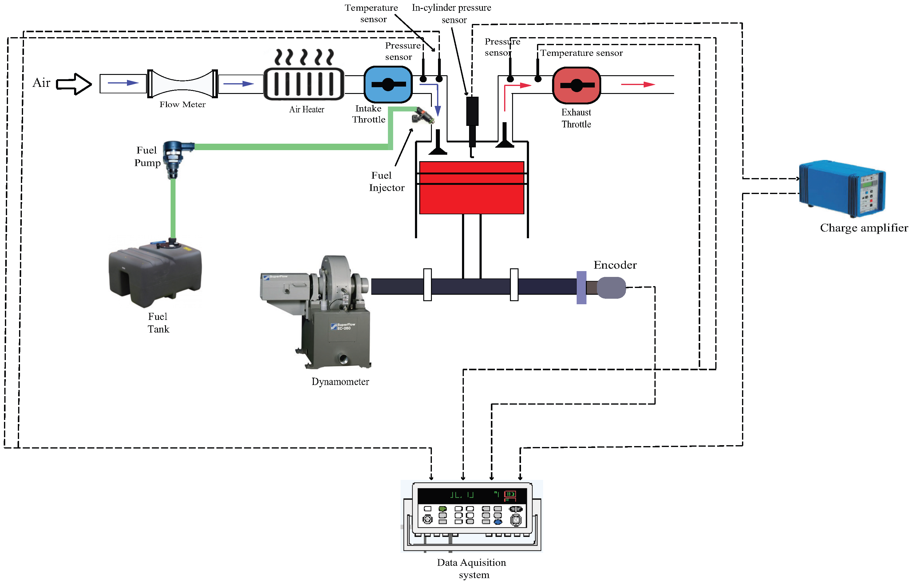
Figure 1 presents the schematic diagram of the experimental setup. The setup includes a 500 cc single-cylinder, 4-stroke, port-injected gasoline engine manufactured by the Taiwan-based company CEC. The engine specifications are provided in Table 1. An air heater (Leister LHS21L) is used to preheat the intake air entering the cylinder. K-type thermocouples are installed at the intake and exhaust manifolds to measure temperature. An intake manifold pressure sensor (SP–Ax102–B) is utilized to measure the pressure within the intake manifold.
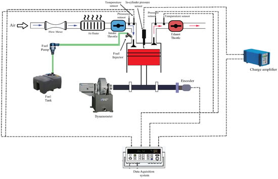
Figure 1.
Schematic diagram of the experimental setup.

Table 1.
Engine Specifications.
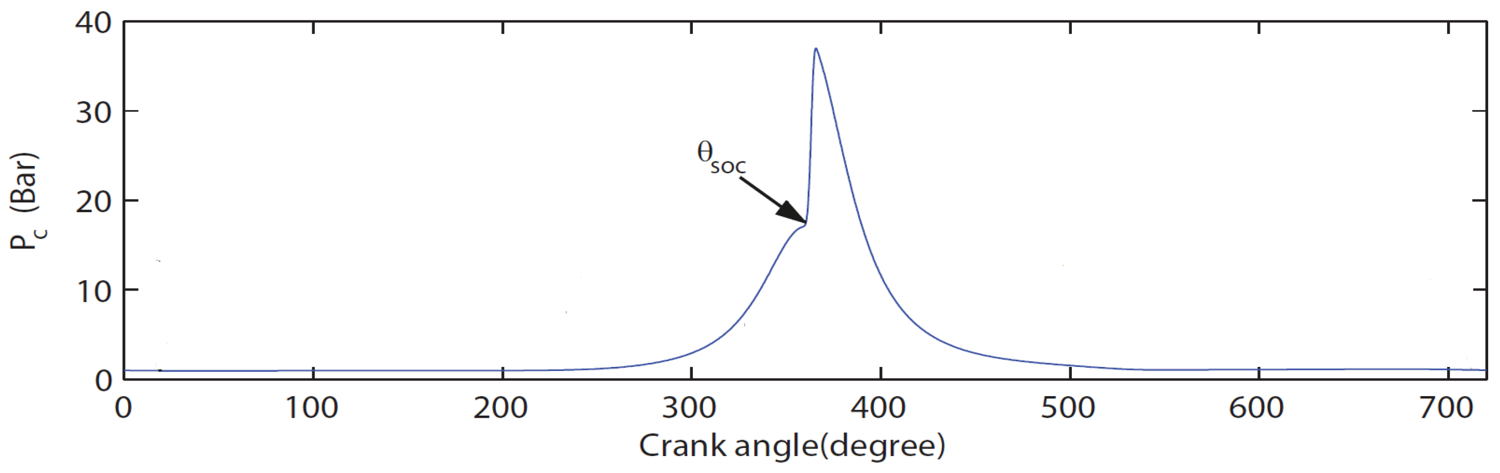
To measure in-cylinder pressure, an AVL spark plug sensor, ZI21U3CPRT, is used in conjunction with a charge amplifier (KISTLER 5011B). The volumetric flow rate of the intake air is recorded using a Schmidt flow sensor SS 30.301, with a measuring range of up to 229 N · 3/hour. The test engine is coupled to an FR 50 eddy current dynamometer with a torque rating of 150 N · and a power rating of 40 kW. An angle encoder (HENGSTLER incremental encoder RI38) is installed to measure the crank angle, with a maximum speed limit of 10,000 rpm. The engine is fueled with 92 AKI unleaded gasoline. Figure 2 illustrates the pressure curve within one cycle, along with the start of combustion timing.
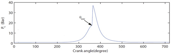
Figure 2.
In-cylinder pressure curve.
2.2. Long Short-Term Memory (LSTM)
First introduced by Hochreiter and Schmidhuber in 1997 [26], LSTMs have proven to be powerful tools for predicting certain outputs from given input data in various domains, such as natural language processing [27], event prediction [28], traffic forecasting [29], and stock market prediction [30]. Recently, LSTMs have also found applications in engine failure prediction. Aydin and Guldamlasioglu [31] collect sensor data to predict engine lifetimes and determine suitable times for engine maintenance. Yuan et al. [32] apply LSTMs to aero engines for performance prediction, testing different LSTM variations on a health monitoring dataset of aircraft turbofan engines provided by NASA. The standard LSTM outperforms other variations.
LSTMs set themselves apart from other machine learning methods due to their memory component, making them particularly useful for time series prediction [33]. LSTMs improve upon other structures, such as recurrent neural networks, by introducing gate functions into the cell [34]. This feature enables them to handle long-term relationships effectively. LSTMs can use inputs from different time steps and employ these inputs for their predictions. When applied to the domain of engine data, LSTMs have previously been used to predict engine failure.
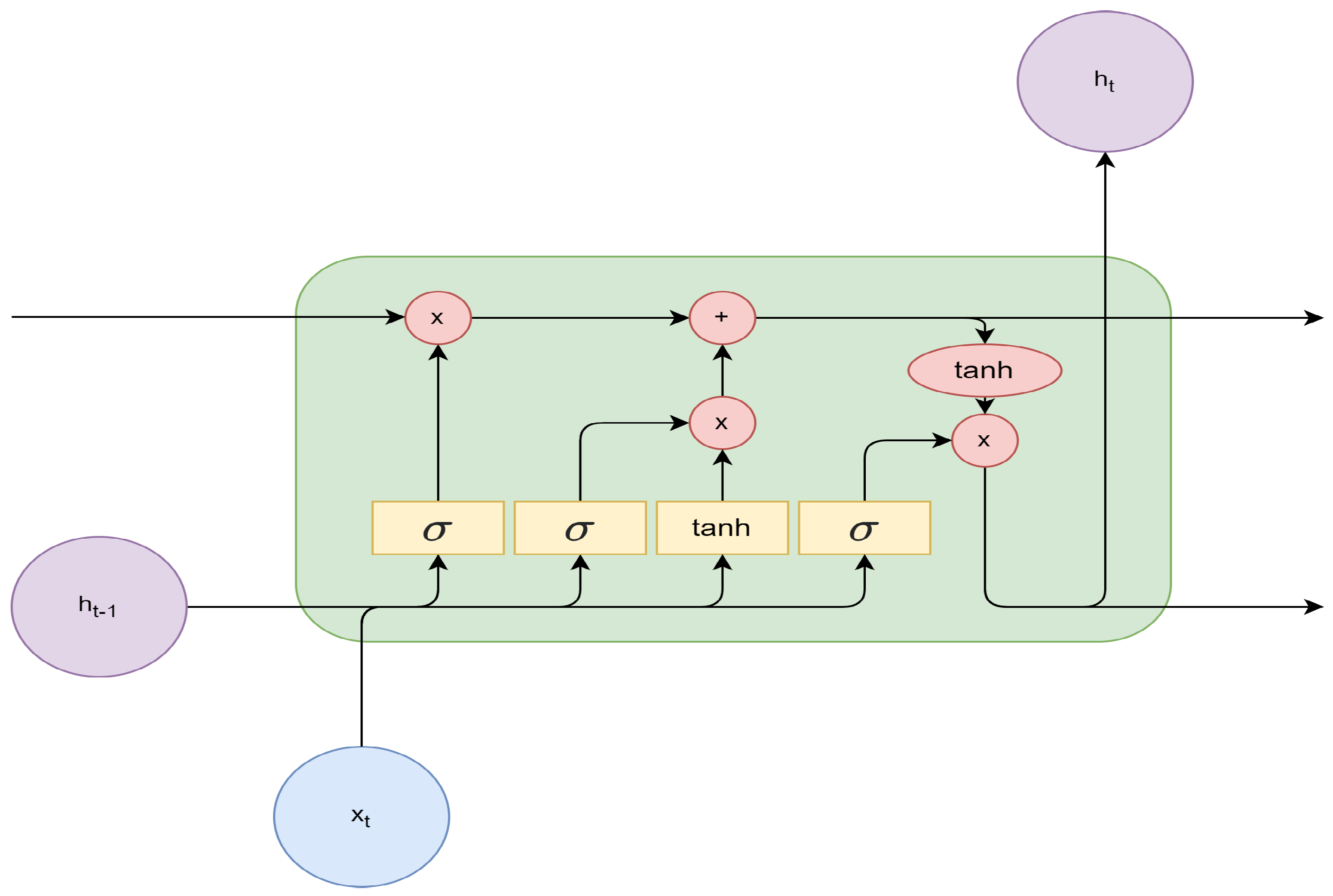
LSTM architectures can vary greatly. A basic building unit of an LSTM is shown in Figure 3. represents the input vector, and denotes the output prediction. Yellow rectangles represent neural network layers, while red circles symbolize pointwise operations, with x standing for multiplication and + representing addition. Black arrows indicate information flow, which can be concatenated in the case of merging vectors or copied in the case of diverging vectors.
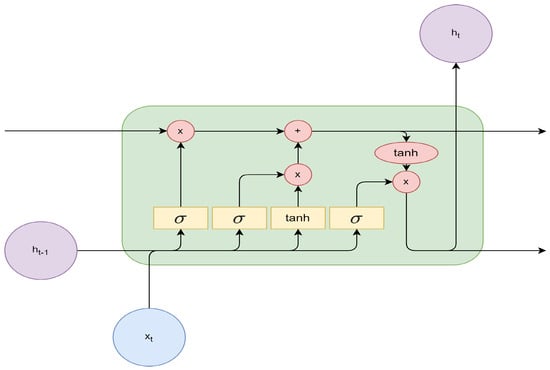
Figure 3.
Basic building unit of LSTM. The previous output and the input vector at time step t are fed into the LSTM building unit and then processed with sigmoid and tanh activation functions and element-wise arithmetic operations. The output is the prediction vector at current time step t.
Figure 3 includes four interacting neural network layers, represented by yellow rectangles. They can be further classified into three sigmoid (abbreviated as in the figure) activation layers and one activation layer. The sigmoid gates output a value between 0 and 1, while the activation function outputs a value between −1 and 1. The gates are also known as the forget, input, and output gates [35]. Each gate has a unique function. The leftmost sigmoid layer is the forget gate, which determines how much of the previous state should be retained. The gate can be described with Equation (1).
where describes the bias at the forget gate.
The next two layers, sigmoid and , form the input gate, which decides about the new information that should be added to the current cell state. Equation (2) presents the sigmoid part of the input gate, while the layer is described in Equation (3). When multiplied together, they are added to the cell state created from the multiplication of the forget gate output and the cell state in Equation (4) to update the current cell state.
Finally, the fourth gate, the output gate, filters the cell state and generates the output. The filter value is created by Equation (7). The filter value is then multiplied with the output of the operation from the current cell state , as seen in Equation (8). The horizontal line at the top represents the cell state.
In summary, the LSTM cell uses forget, input, and output gates to determine how to update its internal cell state and generate output predictions. By handling long-term dependencies and time correlations effectively, LSTMs have been successfully applied to various domains, including engine performance prediction and engine failure prediction [31,32,36].
Equations (7) and (8) describe the output gate of an LSTM cell. represents the sigmoid function , is the tanh function . , , , are the weights of the neural network layer and , , , are the bias vectors. The output gate determines the information that should be output from the cell state. This is done by applying the sigmoid function to the input data and previous hidden state, followed by element-wise multiplication with the tanh of the current cell state.
The performance of the LSTM model is measured using mean average error (MAE) and mean squared error (MSE), as described in Equations (9) and (10). n describes the number of sample points in the test set, is the groundtruth and is the prediction of the machine learning model. These metrics provide a quantifiable way to assess the accuracy of the model’s predictions.
The pressure curve in this study has the characteristics of a time series, where observations are used to predict future pressure states over a defined time interval. More specifically, the input size of the LSTM represents the number of observations that the LSTM receives with the input vector . The output size defined by the output vector of the LSTM is the prediction horizon. The prediction horizon specifies, how many time steps ahead with respect to the latest observation in the input vector are predicted. This makes the LSTM model an appropriate choice for predicting cylinder pressure in HCCI engines. By evaluating the model’s performance using the MAE and MSE metrics, we can assess the effectiveness of the LSTM model and its potential for use in similar applications.
3. Results & Discussion
In this section, the results of the study are organized into three main parts. First, different LSTM configurations are explored for predicting time-series data, including various combinations of input and output sizes and hidden layer sizes. Next, the performance of the LSTM model is compared to that of a DNN. Finally, pressure data points are predicted for future time steps at different intake temperatures.
The experiments are conducted using an 80/20 train/test protocol on a dataset with 1,048,576 measurement points. The first 80% of the measured data is used for training; the last 20% is used for testing. This 2-stage process is a common machine learning practice in most machine learning applications. The training set consists of 838,861 samples, while the test set has 209,715 samples. The training data is only used to train the neural network during the training phase. The hold-out test set is then used for evaluation purposes on unseen data to prove the ability of the neural network to cope with unseen data. The training process spans 10 epochs with MAE and MSE loss and a learning rate of 2 × . The loss function calculates the error between prediction and groundtruth. According to the loss, the weights in the neural network are updated until the loss does not change any more and the network converges during training. Convergence of the models is verified by monitoring the loss curve during training, as illustrated in Figure 4. After the convergence of the loss, the trained neural network can then further be used for inference on test data.
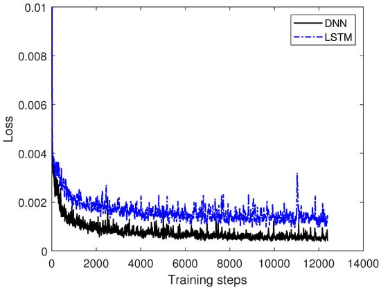
Figure 4.
Training curve of LSTM and DNN during training with data 1 from Table 2. The loss curve of the LSTM is shown in blue; the loss curve of the DNN is shown in black. It can be observed, that the loss of each architecture converges after more than 4000 training steps.
Adam optimization [37] is used during the training process. All experiments were performed on a machine with an Intel® Core™ i7-8700K CPU at 3.70 GHz, 32.00 GB of random access memory, an NVIDIA GeForce GTX™1080 Ti GPU, and a Windows 10 operating system. The PyTorch framework [38] is used for implementing the models.
The results of these experiments will provide insights into the optimal LSTM configuration for predicting cylinder pressure in HCCI engines, as well as a comparison of the LSTM model’s performance to that of a DNN.
3.1. LSTM for Pressure Time-Series Prediction
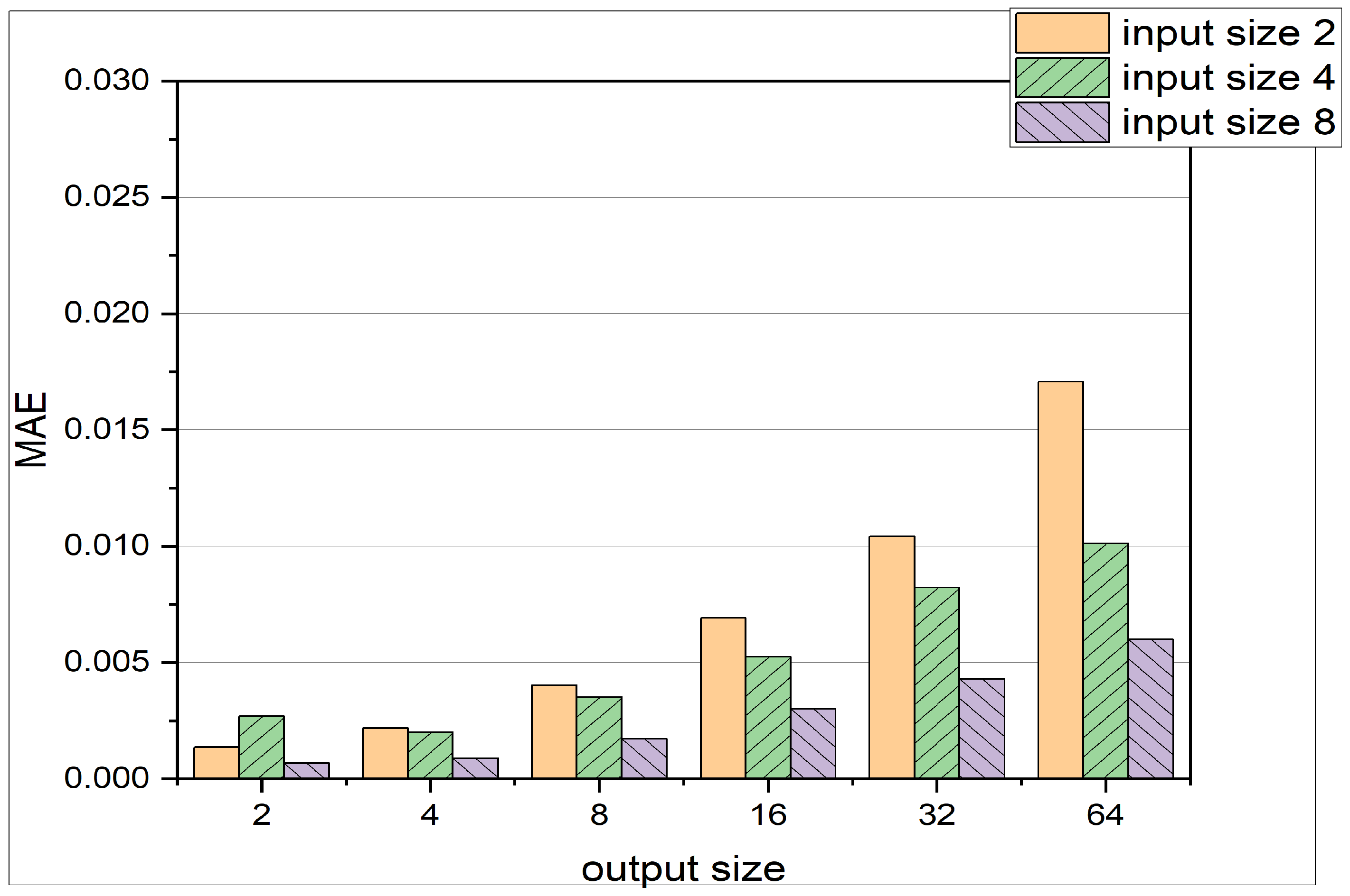
In this initial analysis, the performance of the LSTM architecture is evaluated at different parameters, such as input and output size, hidden layer size, and input features like pressure, temperature, and crank angle. Different configurations of the input and output size of the network produce varying MAE and MSE values, as shown in Table 3 and Figure 5. Several trends can be identified:
Table 3.
Input and output sizes of the LSTM.
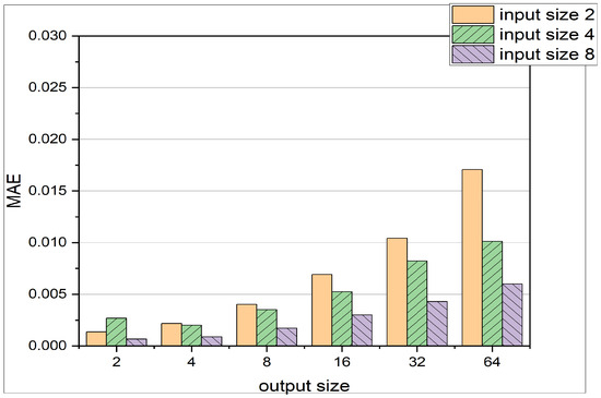
Figure 5.
Comparison of different input sizes and output sizes for LSTM Architecture. The input sizes represent the number of pressure states the LSTM is receiving, whereas the output size represents the dimension of the prediction vector . Exact values are shown in Table 3.
- (a)
- As the input size increases, the MAE and MSE values generally decrease. This trend can be attributed to the fact that a larger input size provides more information to the LSTM, enabling it to make better forecasts.
- (b)
- Conversely, as the output size increases, the MAE and MSE values tend to increase. This outcome occurs because a larger output size corresponds to predictions that are further away from the current time step. For example, when the output size is 64, the LSTM predicts pressure states more than 64 time steps away from the input pressure states. Predicting these distant pressure states accurately becomes more challenging due to the cycle-to-cycle variation of cylinder pressure data.
- (c)
- A comparison of MAE and MSE loss in Figure 6 reveals that the MSE is much smaller than the MAE. This observation indicates that most of the predictions are very close to the actual results, and there are not many outliers. This is due to the fact, that the MSE loss carries a square term, as can be seen in Equation (10). Therefore the MSE loss punishes outliers [39].
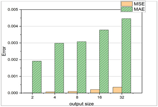 Figure 6. The y-axis represents the MSE respectively the MAE, where the x-axis describes different prediction horizons. The experiment shown is using the test set from data 1 in Table 2.
These findings help to understand how the LSTM architecture’s performance is affected by changes in input and output sizes, and they provide valuable insights for optimizing the model’s configurations for predicting cylinder pressure in HCCI engines. For minimal errors, the LSTM should be fed with the largest input size available. The more data the LSTM receives, the better the predictions. The prediction horizon can be of reasonable size, as long as the MAE is still in the expected and acceptable regime. However, bigger output sizes might lead to higher errors and less precise modeling of the engine pressure.
Table 4 summarizes the MAE and MSE losses at different hidden layer sizes. The hidden layer with 32 neurons shows the best results compared to other cases. Consequently, 32 neurons have been used in the hidden layer of the LSTM in this study.
Table 4.
MAE & MSE results for different hidden layers.
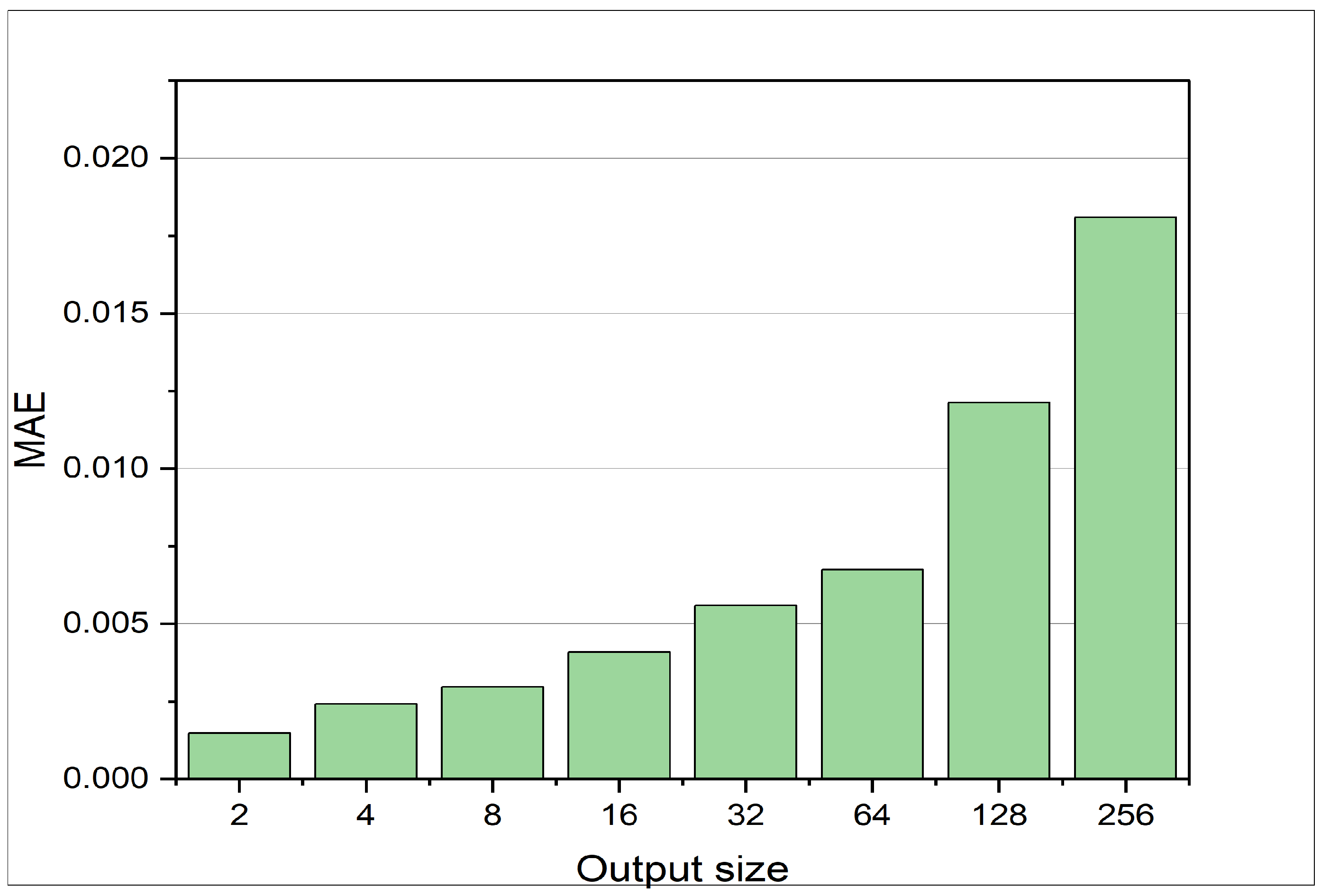
The LSTM’s ability to predict a reasonable number of future pressure states given the current pressure state to is illustrated in Figure 6. k represents the current time step and defines the time step of the latest input. Figure 7 displays the output size of the LSTM within the range of 2 to 256 neurons. Each neuron predicts a distinct time step. As mentioned earlier, the MAE increases with an increase in the output size. The MAE for 256 time steps prediction is below 0.02, given the pressure states from x to .

Figure 7.
MAE at different output sizes for the LSTM. The LSTM is trained on data 2 stated in Table 2. The MAE shown is the error achieved on the test set for the defined test set. With increasing prediction horizon, the error increases.
In the absence of any benchmark for predicting pressure in an engine as a time series, the performance of this study must be evaluated in terms of how well it contributes to research in cylinder pressure modeling. The error in this study is comparable to previous studies [2,10]. To provide a more comprehensive evaluation of the proposed method, the subsequent results will compare it with previously used methods, such as DNN [10].
3.2. Comparison between LSTM and DNN
To evaluate the performance of the LSTM in comparison to the previous study based on DNN [10], experiments are conducted with both DNN and LSTM architectures to gain insight into both methods for the given task of pressure prediction in an HCCI engine. Yacsar et al. [10] use a fully connected neural network with the crank angle and excess air coefficient as input to predict the cylinder pressure as output. Their DNN consists of 3 hidden layers, having 100, 150, and 120 neurons, and employs the ReLU activation function. In the present study, the input is the cylinder pressure of previous time steps to predict the cylinder pressure of current and future time steps for the experiments. The network architecture in this study is compared with the architecture presented by Yacsar et al. [10].
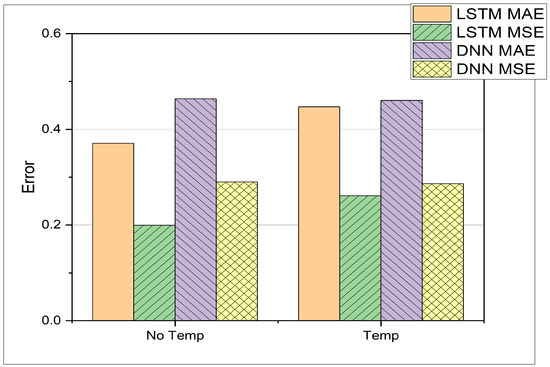
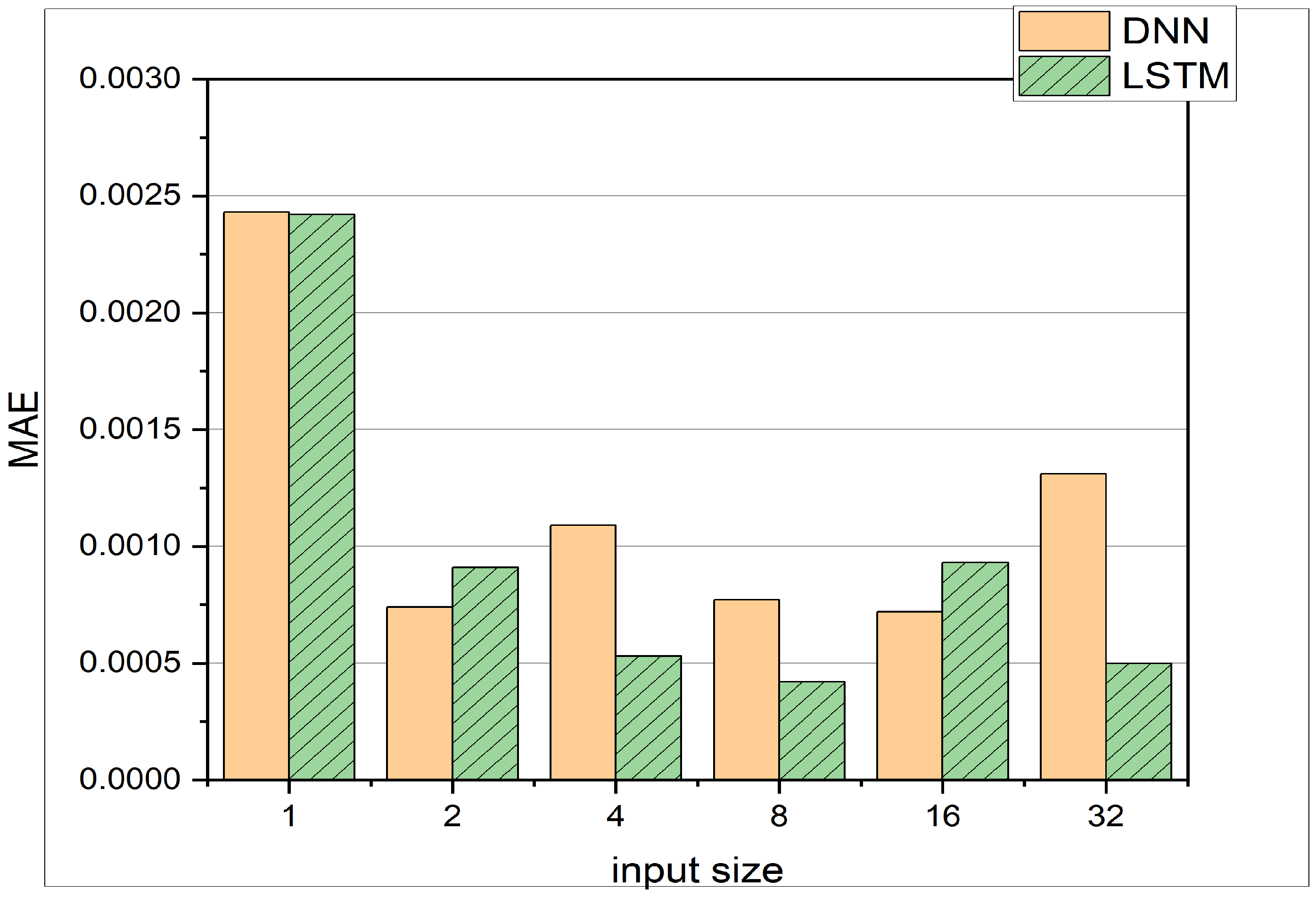
In the present study, the LSTM-based model consists of one hidden layer with 32 neurons. The results can be seen in Table 5 and Figure 8, which depict the comparison between LSTM and DNN. The LSTM yields better results overall with just one hidden layer against the 4 hidden layers in the case of DNN, which results in saving memory and reduced training time. In the previous study, training was found to be optimal for 500 epochs, but in the present study, training for 10 epochs shows comparable results. This might be due to the fact that the size of an epoch can vary. The experiments show that the LSTM can perform better in the scenario of varying input sizes. Each experiment has a different number of input neurons, which can be defined as input size. For the LSTM, the MAE decreases with increasing window size except for the input size of 16. This demonstrates the LSTM’s ability to learn from time series data effectively. It can also be seen that the LSTM outperforms the DNN in 4 out of 6 cases, whereas the DNN only performs better for input sizes of 2 and 16. The DNN is not sensitive to an increasing window size. The test accuracy remains more or less constant between window sizes of 2 and 16. Only for a window size of 1, a much worse performance can be observed. The above comparison is based on the MAE and a constant temperature, whereas in the following experiments, the DNN and LSTM test results are presented at different intake temperatures. Table 6 provides MAE and MSE values for different datasets as defined in Table 2 for both DNN and LSTM architectures. Additionally, the experiments investigate how the two architectures, i.e., DNN and LSTM, cope with different temperature and crank angle as input features. The resulting MAE and MSE are presented in Table 7 and Figure 9. Regarding the computational time given the hardware introduced earlier in Section 3, the LSTM requires 2.73 s of computation during inference on the test set; the DNN requires 3.05 s. The training time of the LSTM is 7 min and 33 s; the training time of the DNN is 6 min and 16 s. Comparing the allocated memory for both architectures, the LSTM occupies 81 Kilobytes of memory space; the DNN occupies 181 Kilobytes. Therefore, it can be said, that the proposed LSTM architecture outperforms the DNN architecture both in inference time and in memory efficiency, even though the training time for the LSTM takes longer.
Table 5.
Results of comparison between DNN and LSTM.
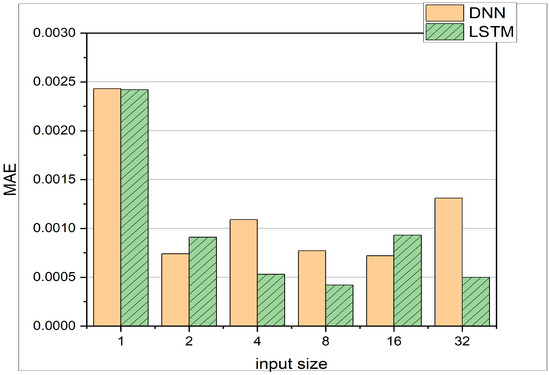
Figure 8.
Comparison of DNN with 4 Layers and the LSTM with 1 Layer. Both networks are trained on the training data 1 from Table 2 and tested on the test data from data 1. The MAE with respect to different input sizes of vector can be observed.
Table 6.
Comparison between DNN and LSTM on predicting pressure at different Temperatures.
Table 2.
Dataset at different temperatures.
Table 7.
Prediction characteristics for Pressure at different Temperature states.
3.3. Intake Temperature
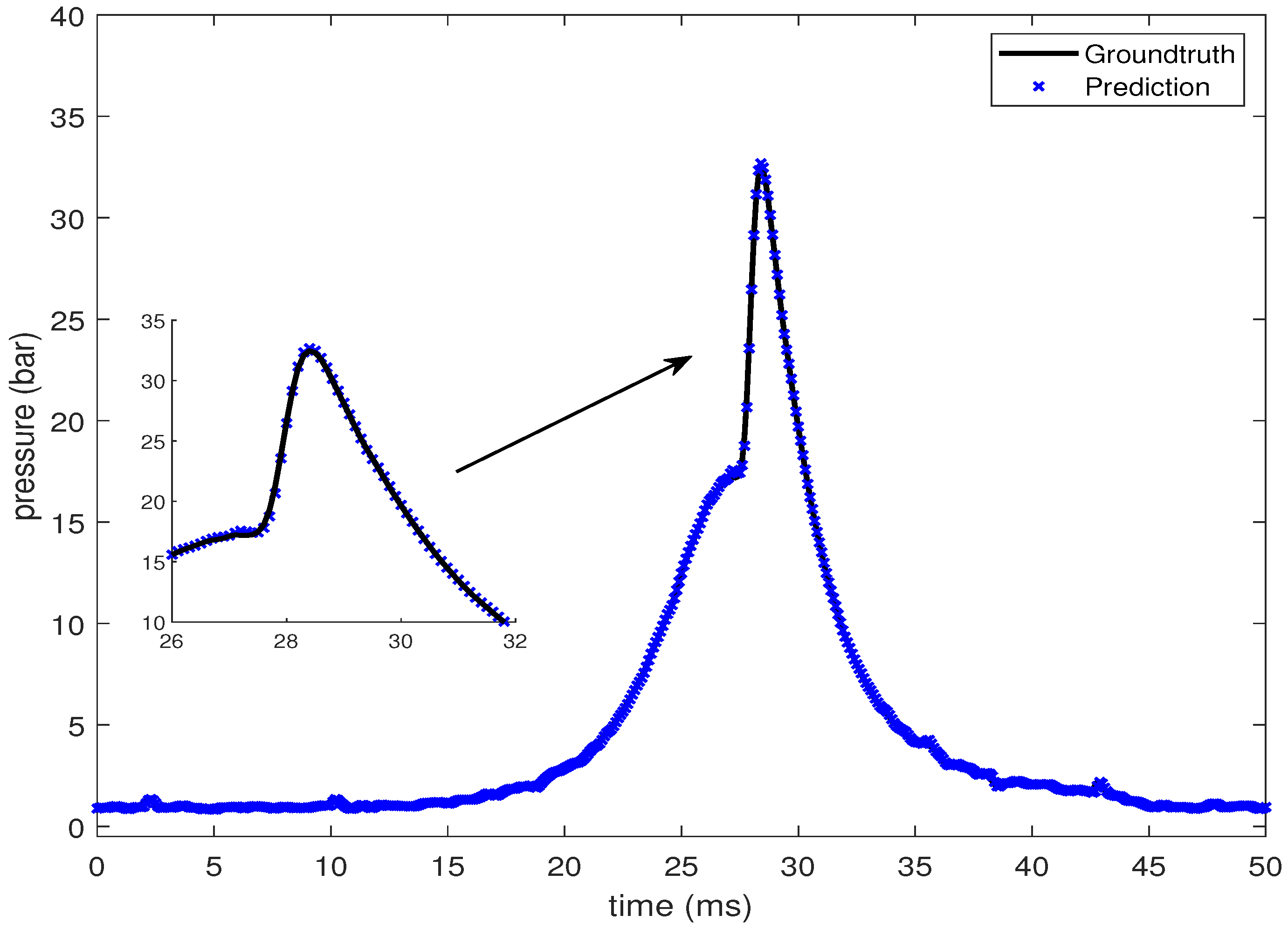
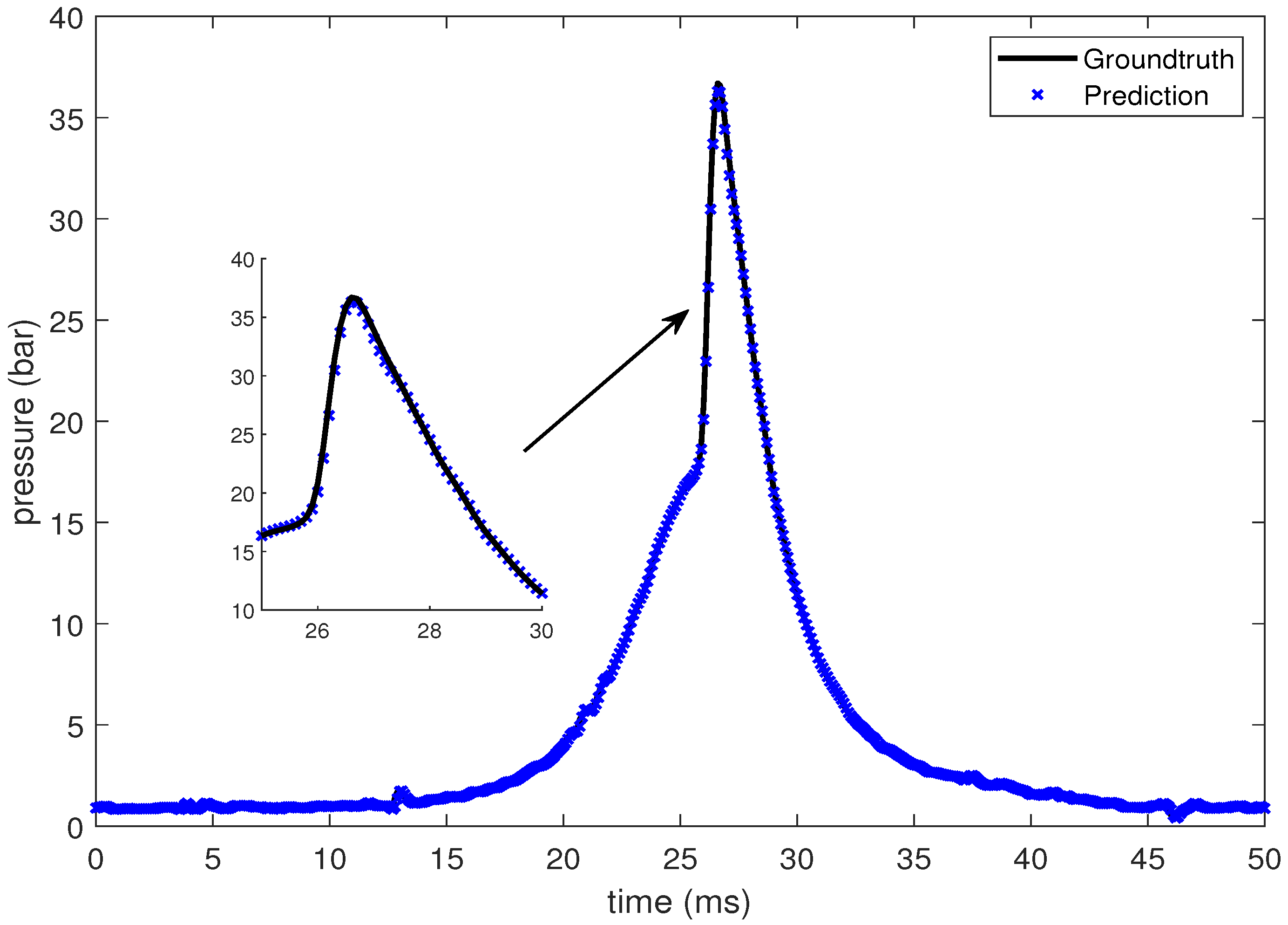
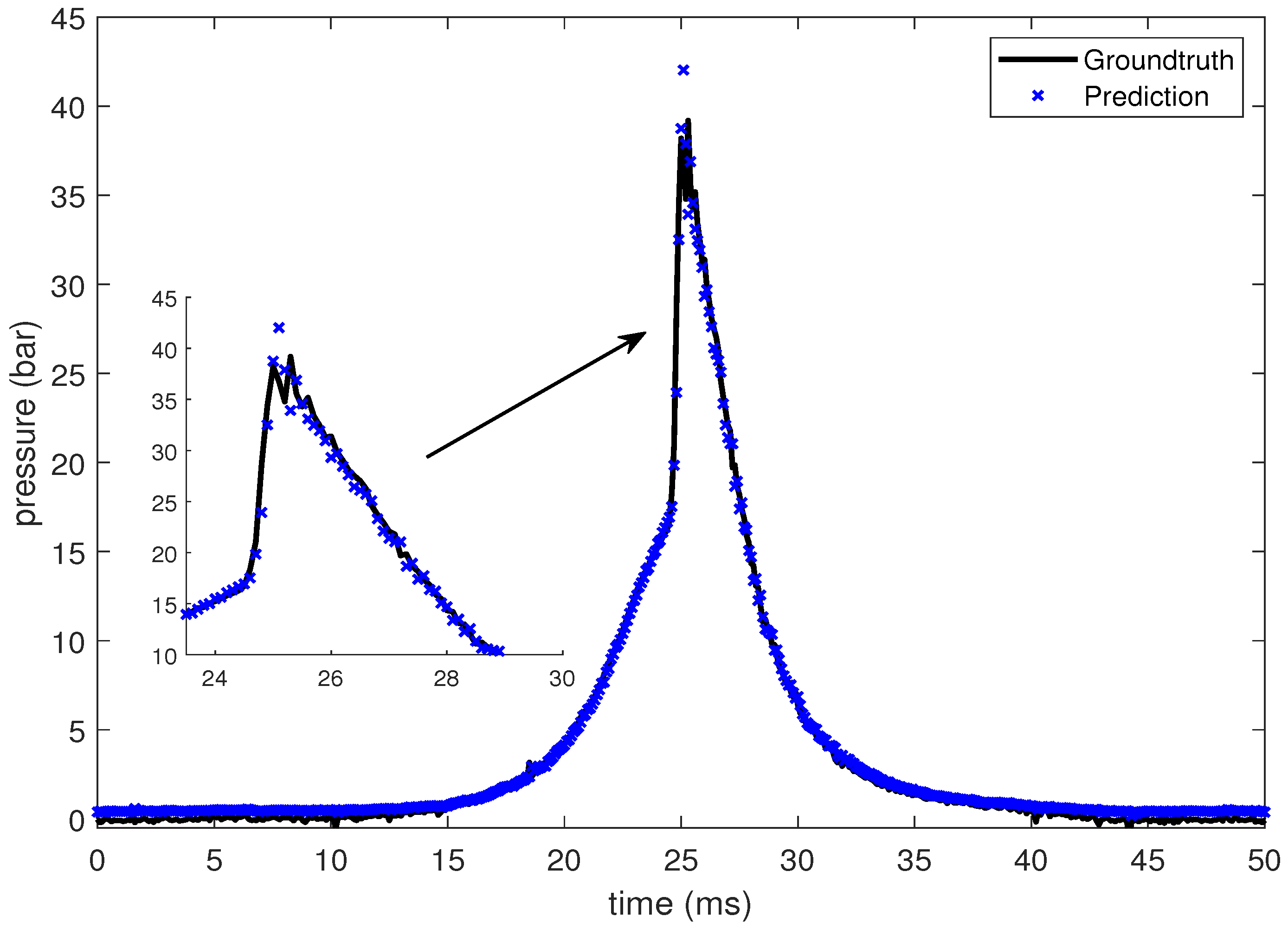
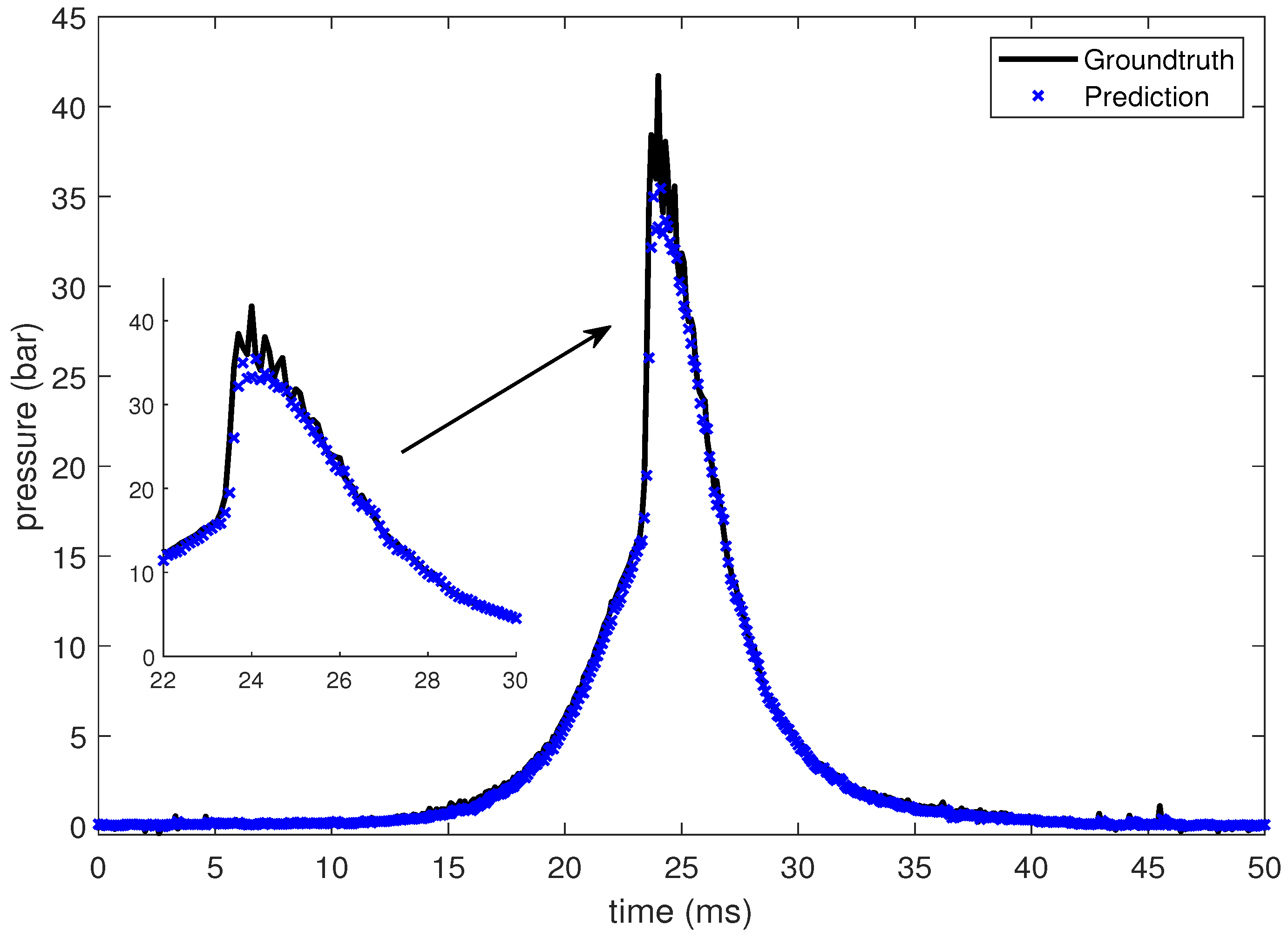
In this section, the LSTM-based prediction of cylinder pressure at different intake temperatures has been presented. Experimental pressure data at different intake temperatures has been recorded and organized as shown in Table 2. The intake temperature is maintained at the desired value using feedback control command to the electrical air heating device introduced in Section 2. The data is then fed into the LSTM-based machine learning model. Pressure data at four different intake temperatures are presented from Figure 10, Figure 11, Figure 12 and Figure 13, which shows that the SOC timing advances with the increase in intake temperature. The results are corroborated by the findings in the study by Chiang et al. [7]. Hence, the suggested LSTM model is capable enough to consider the effect of intake temperatures on one of the combustion characteristics, i.e., SOC. In the case of 235 C intake temperature, the SOC is captured at around 28 ms, as shown in Figure 10. At an intake temperature of 245 C, the SOC timing occurs at around 26 ms in Figure 11, 2 ms earlier than the previous case. The SOC timing advances further to 24.8 ms and 23.9 ms for the remaining two intake temperatures of 255 C and 265 C, respectively, as presented in Figure 12 and Figure 13.
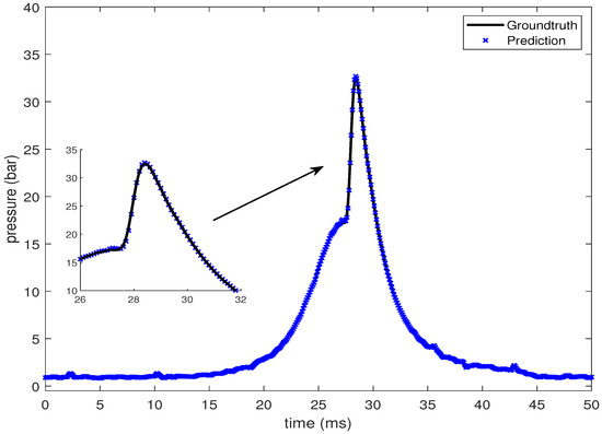
Figure 10.
Groundtruth and prediction data at intake temperature 235 C.
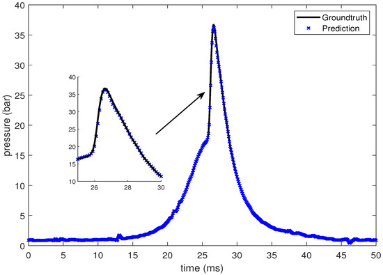
Figure 11.
Groundtruth and prediction data at intake temperature 245 C.
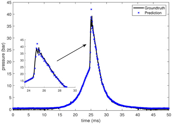
Figure 12.
Groundtruth and prediction data at intake temperature 255 C.
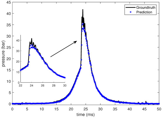
Figure 13.
Groundtruth and prediction data at intake temperature 265 C.
4. Conclusions
In this study, we investigated the application of long short-term memory (LSTM) networks for predicting cylinder pressure in a homogeneous charge compression ignition (HCCI) engine under different operating conditions, specifically intake temperatures. The LSTM model’s performance was analyzed under various configurations, such as input and output sizes and hidden layer sizes. The results demonstrated that the LSTM model could effectively predict cylinder pressure, exhibiting lower mean absolute error (MAE) and mean squared error (MSE) in comparison to a deep neural network (DNN) model with three hidden layers. The accuracy of the LSTM model has been measured on the basis of MAE and MSE. Results shows that for output sizes up to 256, the MAE is below 0.02, which means that the present model can predict 256 time-steps ahead with an acceptable error. Increase in the input size from 2 to 8 results in reduction of the error by up to 50%. The hidden size of 32 gives the best performance in terms of lowest MAE of 0.22 and MSE of 0.049.
Additionally, the LSTM model proved capable of adapting to different window sizes between 4 and 32 and showed better overall performance than the DNN model. For input of different temperatures, the LSTM outperforms the DNN in terms of MAE and MSE. MAE for LSTM is reduced by 20%, on the other hand the MSE for LSTM is reduced by 32% in comparison to DNN for predicting cylinder pressure at different temperatures. The improvement on accuracy is also supported by an improvement on efficiency, since the LSTM requires less than half of the memory space and is faster during inference. Furthermore, the LSTM model successfully captured the impact of intake temperature on the start of combustion (SOC) timing, showcasing its ability to model complex non-linear relationships within the combustion process.
The results presented in this study highlight the potential of LSTM networks in predicting cylinder pressure in HCCI engines, enabling real-time monitoring and control of engine performance. The LSTM model’s ability to handle time-series data and consider the effects of intake temperature on combustion characteristics demonstrates its promise for various applications within the automotive industry. Future work could extend the LSTM model to other engine parameters and investigate its applicability in other combustion engine types. Moreover, exploring the integration of LSTM models with physics-based approaches could provide a more comprehensive understanding of engine performance and enhance the predictive capabilities of these models.
Author Contributions
M.S.: Conceptualization, Methodology, Software. A.-K.S.: Data curation, Writing-original draft preparation, Validation, Writing-Reviewing and Editing, Investigation. P.V.: Visualization, Writing-Reviewing and Editing. S.-Y.C.: Supervision Y.-L.K.: Supervision. All authors have read and agreed to the published version of the manuscript.
Funding
This research was funded by Ministry of Science and Technology (MOST), Taiwan, ROC. Grant number: MOST 109-2221-E-011-069 and NSTC 110-2221-E-011-136-MY3.
Data Availability Statement
The data that support the findings of this study were provided by Ministry of Science and Technology (MOST), but restrictions apply to the availability of these data, which were used under license for the current study, and so are not publicly available. The data is confidential and cannot be disclosed due to the restrictions from the third party.
Acknowledgments
This research was partially supported by the National Science and Technology Council of the Republic of China (Taiwan) under grant NSTC 110-2221-E-011-136-MY3 and the Smart Manufacturing Innovation Center as part of the Featured Areas Research Center Program within the framework of the Higher Education Sprout Project by the Ministry of Education (MOE) in Taiwan. The setup in the present study is provided by the Ministry of Science and Technology (MOST), Taiwan, ROC, under grant no. MOST 109-2221-E-011-069. Also, the authors would like to thanks to Advanced Power and Energy Control (APEC) Laboratory at NTUST for the technical support.
Conflicts of Interest
The authors enumerated in the present study certify that they have no affiliations with or involvement in any organization or entity with any financial or non-financial interest in the subject matter or materials discussed in this manuscript.
Abbreviations
The following abbreviations are used in this manuscript:
| LSTM | Long short term memory |
| SOC | start of combustion |
| HCCI | homogeneous charge compression ignition |
| ANN | artificial neural network |
| SVR | support vector regression |
| RF | random forest |
| GBRT | gradient boosted regression trees |
| WNN | wavelet neural network |
| SGA | stochastic gradient algorithm |
| NARX | non-linear autoregressive with exogenous input |
| KNN | K-nearest neighbors |
| SVM | support vector machines |
| IMEP | indicated mean effective pressure |
| MAE | mean average error |
| MSE | mean squared error |
| DNN | deep neural network |
References
- Fathi, M.; Jahanian, O.; Shahbakhti, M. Modeling and controller design architecture for cycle-by-cycle combustion control of homogeneous charge compression ignition (HCCI) engines—A comprehensive review. Energy Convers. Manag. 2017, 139, 1–19. [Google Scholar] [CrossRef]
- Chiang, C.J.; Singh, A.K.; Wu, J.W. Physics-based modeling of homogeneous charge compression ignition engines with exhaust throttling. Proc. Inst. Mech. Eng. Part D J. Automob. Eng. 2022, 237, 1093–1112. [Google Scholar] [CrossRef]
- Yoon, Y.; Sun, Z.; Zhang, S.; Zhu, G.G. A control-oriented two-zone charge mixing model for HCCI engines with experimental validation using an optical engine. J. Dyn. Syst. Meas. Control 2014, 136, 041015. [Google Scholar] [CrossRef]
- Zeng, X.; Wang, J. A physics-based time-varying transport delay oxygen concentration model for dual-loop exhaust gas recirculation (EGR) engine air-paths. Appl. Energy 2014, 125, 300–307. [Google Scholar] [CrossRef]
- Souder, J.S.; Mehresh, P.; Hedrick, J.K.; Dibble, R.W. A multi-cylinder HCCI engine model for control. In Proceedings of the ASME International Mechanical Engineering Congress and Exposition, Anaheim, CA, USA, 13–19 November 2004; Volume 47063, pp. 307–316. [Google Scholar]
- Hikita, T.; Mizuno, S.; Fujii, T.; Yamasaki, Y.; Hayashi, T.; Kaneko, S. Study on model-based control for HCCI engine. IFAC-PapersOnLine 2018, 51, 290–296. [Google Scholar] [CrossRef]
- Chiang, C.J.; Stefanopoulou, A.G.; Jankovic, M. Nonlinear observer-based control of load transitions in homogeneous charge compression ignition engines. IEEE Trans. Control. Syst. Technol. 2007, 15, 438–448. [Google Scholar] [CrossRef]
- Su, Y.H.; Kuo, T.F. CFD-assisted analysis of the characteristics of stratified-charge combustion inside a wall-guided gasoline direct injection engine. Energy 2019, 175, 151–164. [Google Scholar] [CrossRef]
- Ramesh, N.; Mallikarjuna, J. Evaluation of in-cylinder mixture homogeneity in a diesel HCCI engine—A CFD analysis. Eng. Sci. Technol. Int. J. 2016, 19, 917–925. [Google Scholar] [CrossRef]
- Yaşar, H.; Çağıl, G.; Torkul, O.; Şişci, M. Cylinder pressure prediction of an HCCI engine using deep learning. Chin. J. Mech. Eng. 2021, 34, 7. [Google Scholar] [CrossRef]
- Maass, B.; Deng, J.; Stobart, R. In-Cylinder Pressure Modelling with Artificial Neural Networks; Technical Report, SAE Technical Paper; SAE International: Warrendale, PA, USA, 2011. [Google Scholar]
- Erikstad, S.O. Design patterns for digital twin solutions in marine systems design and operations. In Proceedings of the 17th International Conference Computer and IT Applications in the Maritime Industries COMPIT’18, Pavone, Italy, 14–16 May 2018; pp. 354–363. [Google Scholar]
- LeCun, Y.; Bengio, Y.; Hinton, G. Deep learning. Nature 2015, 521, 436–444. [Google Scholar] [CrossRef]
- Wei, L.; Ding, Y.; Su, R.; Tang, J.; Zou, Q. Prediction of human protein subcellular localization using deep learning. J. Parallel Distrib. Comput. 2018, 117, 212–217. [Google Scholar] [CrossRef]
- Martín, A.; Lara-Cabrera, R.; Fuentes-Hurtado, F.; Naranjo, V.; Camacho, D. Evodeep: A new evolutionary approach for automatic deep neural networks parametrisation. J. Parallel Distrib. Comput. 2018, 117, 180–191. [Google Scholar] [CrossRef]
- Mohammad, A.; Rezaei, R.; Hayduk, C.; Delebinski, T.; Shahpouri, S.; Shahbakhti, M. Physical-oriented and machine learning-based emission modeling in a diesel compression ignition engine: Dimensionality reduction and regression. Int. J. Engine Res. 2022, 24, 904–918. [Google Scholar] [CrossRef]
- Liu, Z.; Liu, J. Machine learning assisted analysis of an ammonia engine performance. J. Energy Resour. Technol. 2022, 144, 112307. [Google Scholar] [CrossRef]
- Jafarmadar, S.; Khalilaria, S.; Saraee, H.S. Prediction of the performance and exhaust emissions of a compression ignition engine using a wavelet neural network with a stochastic gradient algorithm. Energy 2018, 142, 1128–1138. [Google Scholar]
- Gharehghani, A.; Abbasi, H.R.; Alizadeh, P. Application of machine learning tools for constrained multi-objective optimization of an HCCI engine. Energy 2021, 233, 121106. [Google Scholar] [CrossRef]
- Namar, M.M.; Jahanian, O.; Koten, H. The Start of Combustion Prediction for Methane-Fueled HCCI Engines: Traditional vs. Machine Learning Methods. Math. Probl. Eng. 2022, 2022, 4589160. [Google Scholar] [CrossRef]
- Shamsudheen, F.A.; Yalamanchi, K.; Yoo, K.H.; Voice, A.; Boehman, A.; Sarathy, M. Machine Learning Techniques for Classification of Combustion Events under Homogeneous Charge Compression Ignition (HCCI) Conditions; Technical Report, SAE Technical Paper; AE International: Warrendale, PA, USA, 2020. [Google Scholar]
- Janakiraman, V.M.; Nguyen, X.; Assanis, D. Nonlinear identification of a gasoline HCCI engine using neural networks coupled with principal component analysis. Appl. Soft Comput. 2013, 13, 2375–2389. [Google Scholar] [CrossRef]
- Mishra, C.; Subbarao, P. Machine learning integration with combustion physics to develop a composite predictive model for reactivity controlled compression ignition engine. J. Energy Resour. Technol. 2022, 144, 042302. [Google Scholar] [CrossRef]
- Zheng, Z.; Lin, X.; Yang, M.; He, Z.; Bao, E.; Zhang, H.; Tian, Z. Progress in the application of machine learning in combustion studies. ES Energy Environ. 2020, 9, 1–14. [Google Scholar] [CrossRef]
- Luján, J.M.; Climent, H.; García-Cuevas, L.M.; Moratal, A. Volumetric efficiency modelling of internal combustion engines based on a novel adaptive learning algorithm of artificial neural networks. Appl. Therm. Eng. 2017, 123, 625–634. [Google Scholar] [CrossRef]
- Hochreiter, S.; Schmidhuber, J. Long short-term memory. Neural Comput. 1997, 9, 1735–1780. [Google Scholar] [CrossRef]
- Huang, Z.; Xu, W.; Yu, K. Bidirectional LSTM-CRF models for sequence tagging. arXiv 2015, arXiv:1508.01991. [Google Scholar]
- Gers, F.A.; Schraudolph, N.N.; Schmidhuber, J. Learning precise timing with LSTM recurrent networks. J. Mach. Learn. Res. 2002, 3, 115–143. [Google Scholar]
- Zhao, Z.; Chen, W.; Wu, X.; Chen, P.C.; Liu, J. LSTM network: A deep learning approach for short-term traffic forecast. IET Intell. Transp. Syst. 2017, 11, 68–75. [Google Scholar] [CrossRef]
- Chen, K.; Zhou, Y.; Dai, F. A LSTM-based method for stock returns prediction: A case study of China stock market. In Proceedings of the 2015 IEEE International Conference on Big Data (Big Data), Santa Clara, CA, USA, 29 October–1 November 2015; pp. 2823–2824. [Google Scholar]
- Aydin, O.; Guldamlasioglu, S. Using LSTM networks to predict engine condition on large scale data processing framework. In Proceedings of the 2017 4th International Conference on Electrical and Electronic Engineering (ICEEE), Ankara, Turkey, 8–10 April 2017; pp. 281–285. [Google Scholar]
- Yuan, M.; Wu, Y.; Lin, L. Fault diagnosis and remaining useful life estimation of aero engine using LSTM neural network. In Proceedings of the 2016 IEEE International Conference on Aircraft Utility Systems (AUS), Beijing, China, 10–12 October 2016; pp. 135–140. [Google Scholar]
- Shi, Z.; Chehade, A. A dual-LSTM framework combining change point detection and remaining useful life prediction. Reliab. Eng. Syst. Saf. 2021, 205, 107257. [Google Scholar] [CrossRef]
- Yu, Y.; Si, X.; Hu, C.; Zhang, J. A review of recurrent neural networks: LSTM cells and network architectures. Neural Comput. 2019, 31, 1235–1270. [Google Scholar] [CrossRef] [PubMed]
- Lindemann, B.; Müller, T.; Vietz, H.; Jazdi, N.; Weyrich, M. A survey on long short-term memory networks for time series prediction. Procedia CIRP 2021, 99, 650–655. [Google Scholar] [CrossRef]
- Chui, K.T.; Gupta, B.B.; Vasant, P. A genetic algorithm optimized RNN-LSTM model for remaining useful life prediction of turbofan engine. Electronics 2021, 10, 285. [Google Scholar] [CrossRef]
- Kingma, D.P.; Ba, J. Adam: A method for stochastic optimization. arXiv 2014, arXiv:1412.6980. [Google Scholar]
- Paszke, A.; Gross, S.; Massa, F.; Lerer, A.; Bradbury, J.; Chanan, G.; Killeen, T.; Lin, Z.; Gimelshein, N.; Antiga, L.; et al. Pytorch: An imperative style, high-performance deep learning library. In Proceedings of the 33rd Conference on Neural Information Processing Systems (NeurIPS 2019), Vancouver, BC, Canada, 8–14 December 2019. [Google Scholar]
- Körding, K.P.; Wolpert, D.M. The loss function of sensorimotor learning. Proc. Natl. Acad. Sci. USA 2004, 101, 9839–9842. [Google Scholar] [CrossRef] [PubMed]


Disclaimer/Publisher’s Note: The statements, opinions and data contained in all publications are solely those of the individual author(s) and contributor(s) and not of MDPI and/or the editor(s). MDPI and/or the editor(s) disclaim responsibility for any injury to people or property resulting from any ideas, methods, instructions or products referred to in the content. |
© 2023 by the authors. Licensee MDPI, Basel, Switzerland. This article is an open access article distributed under the terms and conditions of the Creative Commons Attribution (CC BY) license (https://creativecommons.org/licenses/by/4.0/).