Design and Analysis of an Adaptive Obstacle-Overcoming Tracked Robot with Passive Swing Arms

Abstract

This paper presents a novel adaptive tracked robot equipped with passive swing arms for overcoming obstacles. First, the paper introduces the overall composition of the robot and focuses on the adaptive mechanism of the passive swing arms. Second, analyzing the single-step obstacle-overcoming process of the robot reveals the relationship between the obstacle height and the geometric parameters of the passive swing arms, establishing a kinematic model. Then, a dynamic model of the robot’s obstacle-overcoming process is established by simplifying the robot into a crank–slider linkage, and the time range for the robot to overcome obstacles is analyzed. Finally, through virtual simulation and a physical prototype, the feasibility and maneuverability of the robot’s design are verified. These findings demonstrate the potential of the robot in various applications, such as search and rescue missions and homeland security.

1. Introduction

Over the past few decades, mobile robots have been developed to meet the increasing demand for completing such tasks as disaster-management activities [1], planetary exploration [2], and agriculture [3] in manifold environments. The wheeled mobile robots have been widely used because of their high speed on regular terrain and simple control systems such as RT-Mover [4] and a passively–actively transformable mobile robot [5]. Otherwise, legged robots show great performance in overcoming obstacles, such as stairs or slippery terrain such as Mini Cheetah [6]. What is more, many researchers proposed some novel legged robots such as a rock-climbing robot [7], a multimimicry quadruped robot [8,9], and a portable off-road crawling hexapod robot [10].

In order to combine the speed of wheeled robots with the obstacle-overcoming ability of legged robots, many researchers studied hybrid wheeled–legged robots. Victor et al. [11] presented a two-wheeled jumping robot, which combines smooth maneuvering on flat ground and dynamic overcoming of obstacles. Marko et al. [12] proposed a wheeled quadrupedal robot capable of executing a hybrid walking–driving locomotion. Zhang et al. [13] designed an untethered, quasi-wheeled hexapod robot, which can perform wheeled-like smooth rides on flat ground and traverse height variations well exceeding its trunk clearance. Otherwise, Chen et al. [14] used a linkage mechanism in the design of a novel two-degrees-of-freedom module capable of transforming its shape between a wheel and a leg. Nevertheless, wheeled–legged robots ensure higher adaptability to all kinds of environments, which makes their mechanism quite complicated because of active control algorithms equipped with additional actuators and sensors [15].

Compared with wheeled robots and legged robots, tracked robots can move fast on uneven and yielding terrains since their contact surface with the ground is much larger than that of the other types [16]. The main limitation of tracked robots is their limited capability to overcome high obstacles, steps, and stairs. Aiming to improve the obstacle-overcoming performance, Yasuhiro et al. [17] designed an internal mechanism to shift the longitudinal position of the robot’s center of gravity. Zong et al. [18] proposed a tracked robot that can overcome obstacles by installing a joint motor to lift up the robot’s front segment. In order to achieve higher obstacle-crossing capability and operative flexibility, an architecture with active flippers is widely studied, which can climb steps by turning the arms at the front and rear of the vehicle actively [19,20,21]. In addition, because of the high adaptability of legged robots, many scholars have studied hybrid tracked–legged robots such as TAlBOT [22] and WheTLHLoc [23]. For the inspection of narrow spaces, some researchers have proposed snake-like tracked robots based on the idea of biomimetic snakes. Examples are the SnakeTrack [24] and RCTR [25]. In addition, modular tracked-robot systems are also researched because of their advantages in versatility, robustness, and manufacturing costs. Liu et al. [26] analyzed the step-climbing process and designed a tracked reconfigurable module robot platform to climb steps by adjusting the pitch angle between two adjacent modules. A multirobot system, composed of tracked modules connected by a parallel manipulator capable of carrying a payload is proposed [27].

Different from the tracked robots that can overcome obstacles by actively adjusting components, researchers have also studied many tracked robots equipped with passive components. Lan and Ma [28] presented a creative idea by designing a crawler mechanism with two locomotion modes, which can move not only on even ground but also on different terrains. Seo et al. [29] proposed a tank-like module-based climbing robot with passive-compliant joints, which can increase adaptability for various moving conditions. Kim et al. [30,31] developed a tracked mobile robot based on the passively articulated suspension structure, which can secure a large contact area between the ground and the driving track.

Most current mobile tracked robots mentioned above need additional motors to drive certain components to overcome obstacles; some tracked robots with passive components also adopt distributed drive solutions using three or more motors. This leads to increased structural complexity, high cost, elevated energy consumption, and heightened control difficulty. To cope with these problems, an adaptive obstacle-overcoming tracked robot is proposed, and a new structure of the main tracked assembly with two passive swing arms is designed. Due to the adoption of two passive swing arms, this proposed robot can achieve functions, such as straight driving, turning, obstacle overcoming, etc., by actuating only two motors. Compared to other tracked robots, the robot can overcome obstacles at a fast speed and has a simple mechanical structure and control system, which reduces the subsequent processing, manufacturing, and maintenance costs.

The paper is organized as follows. In Section 2, the structure design of the robot is described, especially the working principle of passive swing arms. Section 3 provides the kinematic, dynamic analysis, and numerical simulation during the obstacle-overcoming process of the proposed robot. The prototype of the proposed robot is fabricated and validates its effectiveness against steps through physical experiments in Section 4. Section 5 is a discussion and future works. Section 6 concludes the paper.

2. Structure Design of the Robot

2.1. The Composition of the Robot

The adaptive obstacle-overcoming tracked robot with passive swing arms proposed in this paper consists of three main parts, namely, a main tracked assembly, two passive swing arms, and a remote-control unit. As illustrated in Figure 1, the main tracked assembly consists of a chassis, two cameras, two drive wheels, two guide pulleys, and a pair of main tracks wrapping the drive wheels, loading wheels, and cushioning system, which is symmetrically distributed on both sides of the tracked robot, including spring dampers, and carrier rollers.

As shown in Figure 1, two drive wheels are actuated by two servo motors that are installed inside the front segment of the main tracked assembly and attached to the chassis. The battery and the human–robot interaction control system are installed on the inside of the main tracked assembly. In addition, in order to reduce the impact on the robot when it encounters obstacles, four groups of damping modules are arranged on both sides of the main tracked assembly.

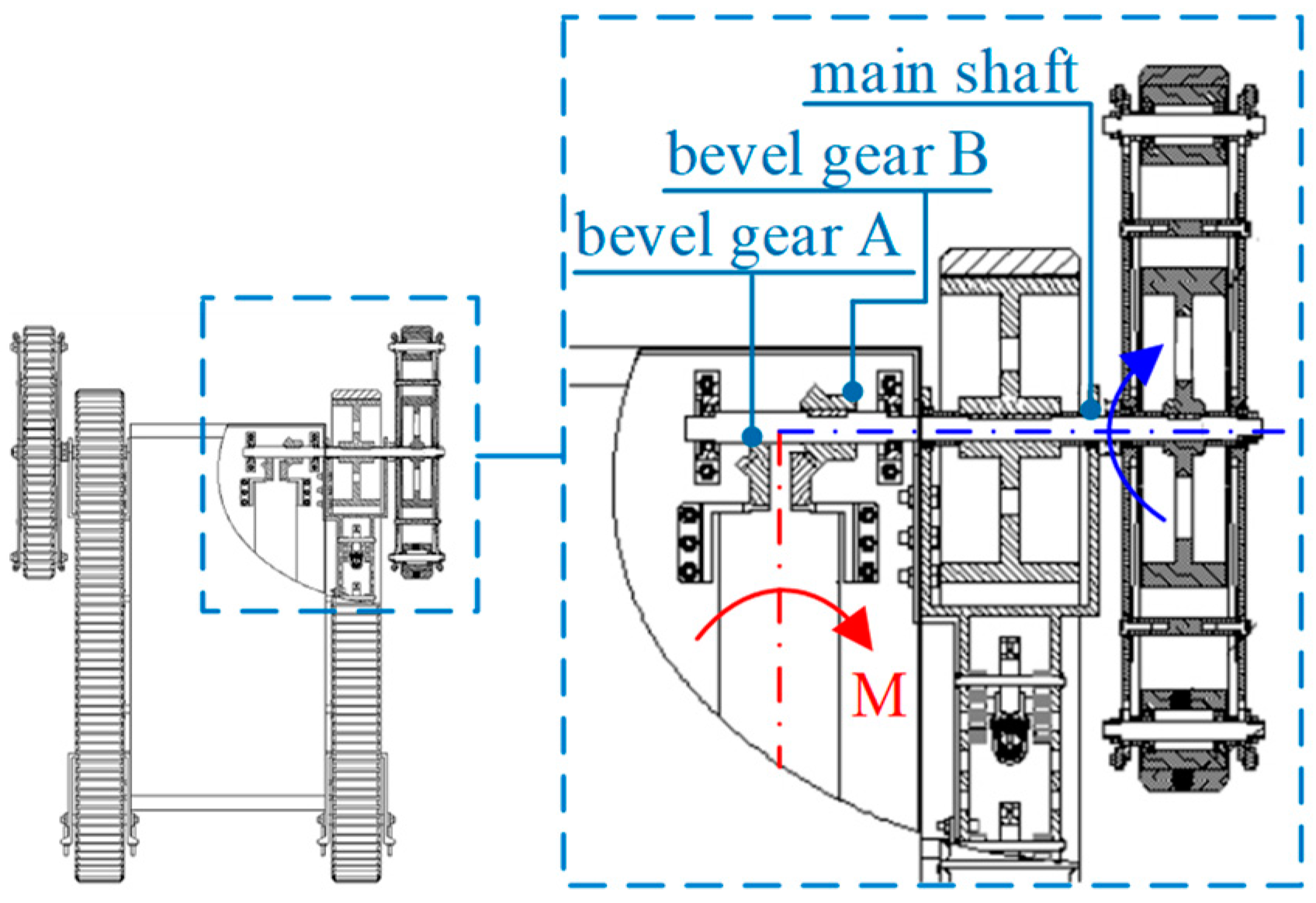
2.2. The Transmission System

As shown in Figure 2, the red arrow represents the torque direction of the motor, and the red dot dash line represents the rotational axis of the motor; The blue arrow represents the direction of rotation of the main shaft, and the blue dot dash line represents the axis of the main shaft. Bevel gear A is connected to the motor through the coupling, and, then, it meshes with bevel gear B for transmission. In addition, bevel gear B is connected to the main shaft through the pin. Under the support of the bearing, the main shaft is connected to the driving wheel, and it is also directly connected to the sun gear of the passive swing arms. As a result, the main shaft drives the driving wheel and sun gear to move simultaneously.

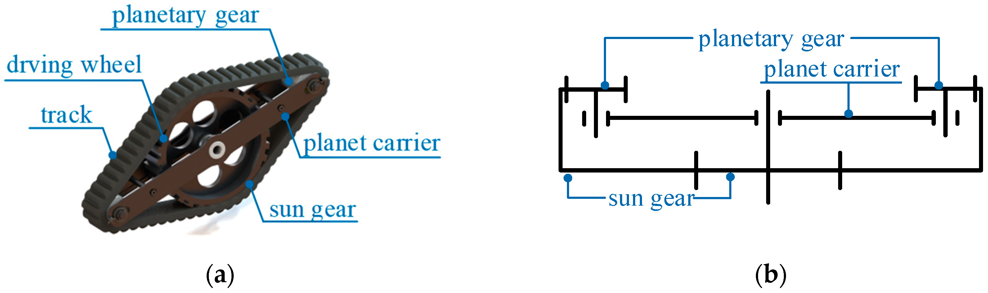
2.3. The Composition and Working Principle of Passive Swing Arms

To enhance the adaptive obstacle-overcoming capabilities, two passive swing arms, powered by two servo motors, are positioned at the front of the tracked robot, as depicted in Figure 1. As shown in Figure 3a, the passive swing arms consist of four parts, a sun gear connecting the drive wheel of the tracked robot, a pair of planetary gears, a planet carrier and a track wrapping the sun gear, and a pair of planetary gears for adapting different obstacles. As shown in Figure 3b, the passive swing arms are essentially a differential gear train. When the sun gear rotates, the outer track rotates to drive the two planetary gears to rotate, which has one degree of freedom; the planet carrier can rotate around the center of the driving wheel, which also has one degree of freedom. Therefore, the whole passive swing arm has two degrees of freedom.

For the entire robot, one main track of the main tracked assembly has one degree of freedom. As shown in Figure 2, one passive swing arm has two degrees of freedom, resulting in a total of six degrees of freedom for the entire robot. However, due to the direct connection between the main shaft and the sun gear, the robot effectively operates with four degrees of freedom, utilizing only two motors. This characteristic design renders the robot an underactuated system with two redundant degrees of freedom, forming the basis for its adaptive obstacle-overcoming capability.

Due to the structural characteristics of the passive swing arms, it has two modes of motion, as shown in Figure 4a, the blue arrow represents the direction of motion of the swing arms, the angle between the planet carrier and the ground can be denoted as α, and the swing arms are in track mode. It is worth noting that this angle remains constant while the tracks of the swing arms rotate around the robot’s drive wheels. In other words, the track of the swing arms conforms closely to the ground. As a result, the contact area between the swing arms and the ground is increased, which can enhance the robot’s ability to traverse on soft surfaces.

When the robot encounters an obstacle, such as the step shown in Figure 4b, the swing arms are in rotation mode, the red arrow represents the direction of motion of the swing arms,; the front ends of the swing arms contact the vertical obstacle first, causing the rotation of the swing-arm tracks to get stuck. At this moment, all components of the swing arms are relatively fixed and can be considered as a whole. The planetary carrier of the swing arms is underactuated, which causes the entire swing arms to flip, resulting in an increase in the angle between the planetary carrier and the ground from α to β. And this is the structural basis for the robot to climb over obstacles.

In the subsequent section, we will place particular emphasis on elucidating the obstacle-overcoming mechanism of the robot. Following that, we will conduct a thorough kinematic and dynamic analysis of the robot’s obstacle-overcoming process.

3. Obstacle-Overcoming Analysis

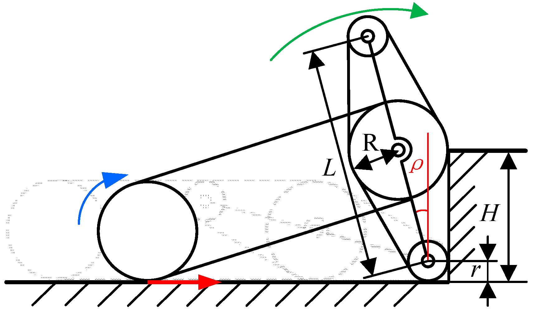
3.1. Kinematic Analysis of Single-Step-Climbing Ability

The robot can move on various terrains, such as flat surfaces and sloped roads. What is more, the robot also possesses a special capability, which is the ability to climb vertical obstacles. Therefore, this chapter focuses on analyzing the motion process of the robot when climbing vertical obstacles. First, it provides a description of the process by which the robot climbs a step. Through the analysis of the obstacle-overcoming process, we have unveiled the geometric relationship between the parameters of the passive swing arm and the height of the obstacle. Furthermore, a kinematic model of the robot’s step climbing using the passive swing arms has been established.

Figure 5 is the illustration of the robot climbing a single step. The blue arrow indicates the direction of rotation of the main track, the red arrow indicates the direction of friction applied to the robot, and the green arrow indicates the direction of rotation of the swing arms during obstacle overcoming. In the initial stage, the robot travels on flat terrain. The main tracks of the robot rotate under the drive of the motors. As a result, the ground provides the robot with frictional force. As the robot continues to move forward, the swing arms make initial contact with the vertical surface of the step, as shown by the dashed line in the diagram. Subsequently, the swing arms pivot. When the swing arms align with the vertical surface of the step, as illustrated in the solid line of the diagram, the robot’s body is elevated. With the effect of frictional force, the robot crosses the step, successfully overcoming the obstacle.

Consequently, it can be observed that the maximum height of the obstacle clearance primarily depends on the length of the passive swing arms. Analysis shows that the relationship between the height of obstacle H and the length of the passive swing arms L can be described by Equation (1). Then, the mesh gird of H with L and r is drawn in Figure 6. By considering the height of common steps, the radius of the driving wheel R is set as 150 mm, the range of L is set as [300, 400] and the range of r is set as [300, 400] in mesh grids.

$$H=r+\frac{L}{2}\cos \rho$$

(1)

According to the obstacle-overcoming process, the maximum torque is required for the swing arms to transition from a horizontal state to a vertical state. We consider the main track as a connecting rod, the rocker arm as a crank, and the rolling point between the rear track and the ground as a slider sliding along the ground. Therefore, the robot can be simplified into a four-bar mechanism, as illustrated in Figure 7.

There are three parts of the mechanism. Bar 1, with a mass of m₁, has a length of r. Bar 2, with a mass of m₂, has a length of l. Slider 3 has a mass of m₃. The coordinate XY of reference is established, as shown in Figure 7. θ is the angle between the crank and the X-axis, which represents the crank angle; ϕ is the angle between the connecting rod and the X-axis. M is the torque applied to the crank, while F is the force acting on the slider (assuming the acceleration due to gravity is g).

The force F in Figure 7 is the driving force generated by the friction between the slider and the ground. In other words, if we assume the coefficient of friction between the slider and the ground is μ, then the magnitude of F will not exceed μmg, where m represents the mass of the slider.

Assuming the center of mass of rod 1 is at the connection between one and two, rod 2 is homogeneous. The physical model of the crank–slider mechanism is shown in Figure 7. The geometric positions of the centers of mass of the crank, connecting rod, and slider are analyzed in the OXY plane, as follows:

$$\{\begin{array}{c}{x}_1=r·\mathrm{c}\mathrm{o}\mathrm{s}\theta ,\hspace{1em}\hspace{1em}{y}_1=r·\mathrm{s}\mathrm{i}\mathrm{n}\theta \\ x_2=r·\mathrm{c}\mathrm{o}\mathrm{s}\theta +\frac{1}{2}·l·\mathrm{c}\mathrm{o}\mathrm{s}\varphi ,\hspace{1em}\hspace{1em}{y}_2=\frac{1}{2}·l·\mathrm{s}\mathrm{i}\mathrm{n}\varphi \\ x_3=r·\mathrm{c}\mathrm{o}\mathrm{s}\theta +l·\mathrm{c}\mathrm{o}\mathrm{s}\varphi ,\hspace{1em}\hspace{1em}{y}_3=0\end{array}$$

(2)

The constraint can be expressed as:

$$r·\sin \theta =l·\sin \varphi$$

(3)

$$\varphi =\arcsin \left(\frac{r}{l}·\sin \theta \right)$$

(4)

Taking the first and second derivatives of the center of mass coordinates of the crank, connecting rod, and slider with respect to time yields, their velocities, and accelerations are:

$$\{\begin{array}{c}{\dot{x}}_1=-r\dot{\theta }\left(t\right)\mathrm{s}\mathrm{i}\mathrm{n}\theta ,\hspace{1em}\hspace{1em}{\dot{y}}_1=r\dot{\theta }\left(t\right)\mathrm{c}\mathrm{o}\mathrm{s}\theta \\ {\dot{x}}_2=-r\dot{\theta }\left(t\right)\mathrm{s}\mathrm{i}\mathrm{n}\theta -\frac{1}{2}·l·\dot{\varphi }\left(t\right)·\mathrm{s}\mathrm{i}\mathrm{n}\varphi ,\hspace{1em}\hspace{1em}{\dot{y}}_2=\frac{1}{2}·l·\dot{\varphi }\left(t\right)·cos\varphi \\ {\dot{x}}_3=-r·\dot{\theta }\left(t\right)·\mathrm{s}\mathrm{i}\mathrm{n}\theta -l·\dot{\varphi }\left(t\right)·\mathrm{s}\mathrm{i}\mathrm{n}\varphi \end{array}$$

(5)

$$\left\{\begin{array}{c}{\ddot{x}}_1=-r·\ddot{\theta }\left(t\right)·\sin \theta -r{\left[\dot{\theta }\left(t\right)\right]}^2\cos \theta ,{\ddot{y}}_1=r·\ddot{\theta }\left(t\right)·\cos \theta -r·{\left[\dot{\theta }\left(t\right)\right]}^2·\sin \theta \\ {\ddot{x}}_2=-r·\ddot{\theta }\left(t\right)·\sin \theta -r{\left[\dot{\theta }\left(t\right)\right]}^2\cos \theta -\left(l·\ddot{\varphi }·\mathrm{s}\mathrm{i}\mathrm{n}\varphi +l{·\left[\dot{\varphi }\left(t\right)\right]}^2·\mathrm{c}\mathrm{o}\mathrm{s}\varphi \right)/2\\ {\ddot{y}}_2=l\left(\ddot{\varphi }\mathrm{c}\mathrm{o}\mathrm{s}\varphi -{\left[\dot{\varphi }\left(t\right)\right]}^2\mathrm{s}\mathrm{i}\mathrm{n}\varphi \right)/2\\ {\ddot{x}}_3=-r·\ddot{\theta }\left(t\right)·\mathrm{s}\mathrm{i}\mathrm{n}\theta -r{\left[\dot{\theta }\left(t\right)\right]}^2·\mathrm{c}\mathrm{o}\mathrm{s}\theta -l·\ddot{\varphi }·\mathrm{s}\mathrm{i}\mathrm{n}\varphi -l·{\left[\dot{\varphi }\left(t\right)\right]}^2·\mathrm{c}\mathrm{o}\mathrm{s}\varphi \end{array}\right.$$

(6)

The slider only moves along the X-axis, so its velocity and acceleration in the Y direction are both zero. This can be derived from Equation (4):

$$\dot{\varphi }=\frac{r·\cos \left[\theta \left(t\right)\right]·\dot{\theta }\left(t\right)}{l\sqrt{1-\frac{r^2·\sin {\left[\theta \left(t\right)\right]}^2}{l^2}}}$$

(7)

$$\ddot{\varphi }=\frac{r^3·\cos {\left[\theta \left(t\right)\right]}^2·\sin \left[\theta \left(t\right)\right]·{\left[\dot{\theta }\left(t\right)\right]}^2}{l^3{\left(1-\frac{r^2·\sin {\left[\theta \left(t\right)\right]}^2}{l^2}\right)}^{3/2}}-\frac{r·\sin \left[\theta \left(t\right)\right]·{\left[\dot{\theta }\left(t\right)\right]}^2}{l\sqrt{1-\frac{r^2·\sin {\left[\theta \left(t\right)\right]}^2}{l^2}}}+\frac{r·\cos \left[\theta \left(t\right)\right]·\ddot{\theta }\left(t\right)}{l\sqrt{1-\frac{r^2·\sin {\left[\theta \left(t\right)\right]}^2}{l^2}}}$$

(8)

The constraint can be expressed as:

$$\Phi \left(Q\right)=r·\sin \theta -l·\sin \varphi =0$$

(9)

where $Q={\left[\varphi ,\theta \right]}^T$ is the generalized coordinate.

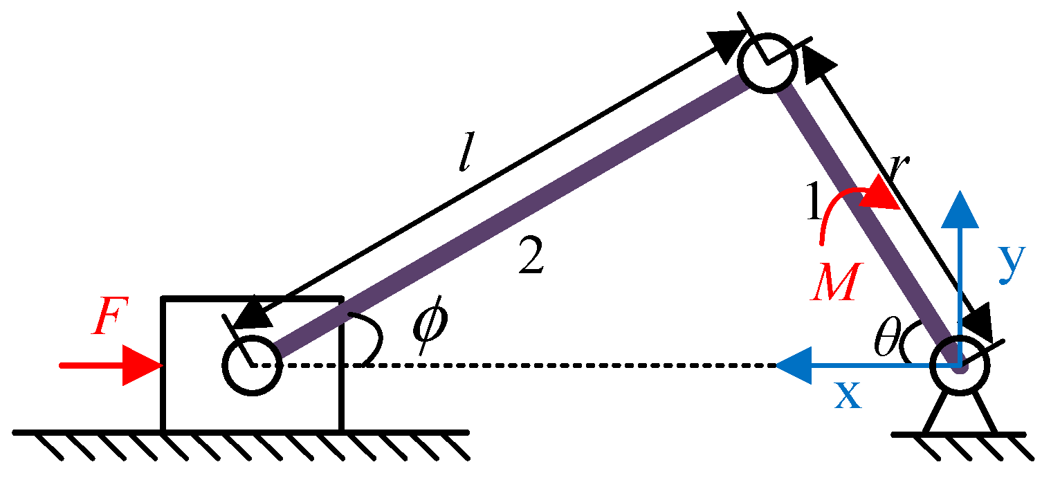
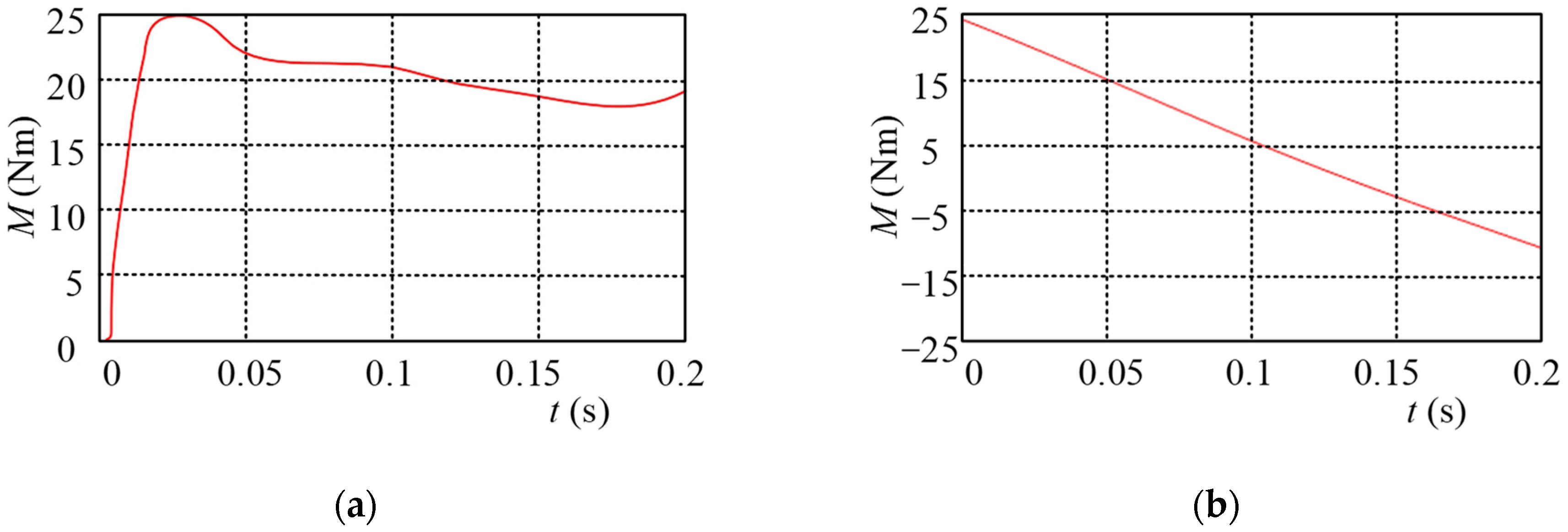
3.2. Dynamic Analysis of Single-Step Climbing

To perform a dynamic analysis of the obstacle-overcoming process, we establish the dynamic model of the robot during the obstacle-overcoming procedure. Subsequently, the torque distribution and optimization are carried out.

The kinetic energy can be expressed as:

$$T_1=\frac{1}{2}·I_1·{\left[\dot{\theta }\left(t\right)\right]}^2=\frac{1}{2}·\left(\frac{1}{3}{m}_1{r}^2\right)·{\left[\dot{\theta }\left(t\right)\right]}^2=\frac{1}{6}·m_1·r^2{\left[\dot{\theta }\left(t\right)\right]}^2$$

(10)

where $I_1=\frac{1}{3}·m_1·r^2\left(kg·m^2\right).$

$$T_2=\frac{1}{2}·I_2·{\left[\dot{\varphi }\left(t\right)\right]}^2+\frac{1}{2}·m_2·{\dot{x}}_2{}^2+\frac{1}{2}·m_2·{\dot{y}}_2{}^2=\frac{1}{6}{m}_2{l}^2{\left[\dot{\varphi }\left(t\right)\right]}^2+\frac{1}{2}{m}_2{r}^2{\left[\dot{\theta }\left(t\right)\right]}^2{\left(\sin \mathsf{\theta }\right)}^2+\frac{1}{2}·m_2·r·l·\dot{\theta }\left(t\right)·\dot{\varphi }\left(t\right)·\sin \theta ·\sin \varphi$$

(11)

where $I_2=\frac{1}{12}{m}_2{l}^2\left(kg·m^2\right).$

$$T_3=\frac{1}{2}·m_3·{\dot{x}}_3{}^2=\frac{1}{2}·m_3·r^2·{\left[\dot{\theta }\left(t\right)\right]}^2{\left(\sin \mathsf{\theta }\right)}^2+m_3·r·l·\dot{\theta }\left(t\right)·\dot{\varphi }\left(t\right)·\sin \theta ·\sin \varphi +\frac{1}{2}·m_3·l^2{\left[\dot{\varphi }\left(t\right)\right]}^2·{\left(\sin \varphi \right)}^2$$

(12)

The potential energy of gravity can be expressed as:

$$\{\begin{array}{c}{V}_1=m_1·g·y_1=m_1·g·r·\mathrm{s}\mathrm{i}\mathrm{n}\theta \\ V_2=m_2·g·y_2=\frac{1}{2}·m_2·g·l·\mathrm{s}\mathrm{i}\mathrm{n}\varphi \\ V_3=0\\ V_4=F\cdot x_3=F\cdot \left(r\cos \theta +l\sin \varphi \right)\\ V_5=-M\cdot \theta \end{array}$$

(13)

Virtual work ${\displaystyle \sum }\delta W$ can be expressed as:

$${\displaystyle \sum }\delta W=M·\delta \theta +F·\delta x=M·\delta \theta +F\left(-r·\sin \theta ·\delta \theta -l·\sin \varphi ·\delta \varphi \right)$$

(14)

Substituting Equation (4) into the above equation yields:

$${\displaystyle \sum }\delta W=M·\delta \theta +F·\delta x=M·\delta \theta +F\left(-r·\sin \theta ·\delta \theta -\frac{r^2·\cos \theta }{\sin \theta \sqrt{1-\frac{r^2·{\left(\sin \mathsf{\theta }\right)}^2}{l^2}}}·\delta \theta \right)$$

(15)

where $\delta \varphi =\frac{r·\cos \theta }{l\sqrt{1-\frac{r^2·{\left(\sin \mathsf{\theta }\right)}^2}{l^2}}}·\delta \theta$.

$Q_{\theta }$ can be expressed as:

$$Q_{\theta }=M+F\left(-r·\sin \theta -\frac{r^2·\cos \theta }{\sin \theta \sqrt{1-\frac{r^2·{\left(\sin \mathsf{\theta }\right)}^2}{l^2}}}\right)$$

(16)

where $F\le \mu m_{3}g$.

By eliminating $\varphi$ and $\dot{\varphi }$ using the relationship between $\theta$ and $\varphi$, T₁ and T₃ can be obtained:

$$T_1=\frac{1}{2}·I_1·{\left[\dot{\theta }\left(t\right)\right]}^2=\frac{1}{2}\left(\frac{1}{3}{m}_1{r}^2\right){\left[\dot{\theta }\left(t\right)\right]}^2=\frac{1}{6}{m}_1{r}^2{\left[\dot{\theta }\left(t\right)\right]}^2=0.02{\left[\dot{\theta }\left(t\right)\right]}^2$$

(17)

$$T_2=\frac{1}{2}{I}_2{\left[\dot{\varphi }\left(t\right)\right]}^2+\frac{1}{2}{m}_2{\dot{x}}_2{}^2+\frac{1}{2}{m}_2{\dot{y}}_2{}^2=10{\left(-0.2·\sin \left[\theta \left(t\right)\right]·\dot{\theta }\left(t\right)-\frac{0.033·\cos \left[\theta \left(t\right)\right]·\sin \left[\theta \left(t\right)\right]·\dot{\theta }\left(t\right)}{\sqrt{1-\theta .11·\sin {\left[\theta \left(t\right)\right]}^2}}\right)}^2$$

(18)

$$T_3=\frac{1}{2}{m}_3{\dot{x}}_3{}^2=\frac{7}{2}{\left(-0.2·\sin \left[\theta \left(t\right)\right]·\dot{\theta }\left(t\right)-\frac{0.067·\cos \left[\theta \left(t\right)\right]·\sin \left[\theta \left(t\right)\right]\dot{·\theta }\left(t\right)}{\sqrt{1-0.11·\sin {\left[\theta \left(t\right)\right]}^2}}\right)}^2$$

(19)

Potential energy can be expressed as:

$$\{\begin{array}{c}{V}_1=m_1·g·y_1=m_1·g·r·\sin \left[\theta \left(t\right)\right]\\ V_2=m_2·g·y_2=\frac{1}{2}·m_2·g·l·\sin \varphi =\frac{1}{2}·m_2·g·r·\sin \left[\theta \left(t\right)\right]\\ V_3=0\\ V_4=Fr\left[\cos \left[\theta \left(t\right)\right]+\sin \left[\theta \left(t\right)\right]\right]\\ V_5=-M\cdot \theta \left(t\right)\end{array}$$

(20)

T can be expressed as:

$$\begin{gathered} T=0.02·{\left[\dot{\theta }\left(t\right)\right]}^2+0.1·\cos {\left[\theta \left(t\right)\right]}^2·{\left[\dot{\theta }\left(t\right)\right]}^2+\frac{0.03·\cos {\left[\theta \left(t\right)\right]}^2{\left[\dot{\theta }\left(t\right)\right]}^2}{1-0.11·\sin {\left[\theta \left(t\right)\right]}^2}+ \\ \frac{7}{2}{\left(-0.2·\sin \left[\theta \left(t\right)\right]·\dot{\theta }\left(t\right)-\frac{0.067·\cos \left[\theta \left(t\right)\right]·\sin \left[\theta \left(t\right)\right]\dot{\theta }\left(t\right)}{\sqrt{1-0.11·\sin {\left[\theta \left(t\right)\right]}^2}}\right)}^2+ \\ 10{\left(-0.2·\sin \left[\theta \left(t\right)\right]\dot{\theta }\left(t\right)-\frac{0.033·\cos \left[\theta \left(t\right)\right]·\sin \left[\theta \left(t\right)\right]\dot{·\theta }\left(t\right)}{\sqrt{1-0.11·\sin {\left[\theta \left(t\right)\right]}^2}}\right)}^2 \end{gathered}$$

(21)

The total potential energy can be expressed as:

$$\begin{gathered} V=V_1+V_2+V_3+V_4+V_5=m_1·g·r·\sin \theta +\frac{1}{2}·m_2·g·r·\sin \theta +F·r·\left(\cos \theta +\sin \theta \right)-M·\theta \left(t\right) \\ =26\cdot \sin \left[\theta \left(t\right)\right]+F\cdot \left(0.2·\cos \left[\theta \left(t\right)\right]+0.6\sqrt{1-0.11·\sin {\left[\theta \left(t\right)\right]}^2}\right)-M\cdot \theta \left(t\right) \end{gathered}$$

(22)

$$\begin{array}{c}L=T-V=-26\cdot \mathrm{s}\mathrm{i}\mathrm{n}\left[\theta \left(t\right)\right]-F\cdot \left(0.2·\mathrm{c}\mathrm{o}\mathrm{s}\left[\theta \left(t\right)\right]+0.6\sqrt{1-0.11·\mathrm{s}\mathrm{i}\mathrm{n}{\left[\theta \left(t\right)\right]}^2}\right)\\ +M\cdot \theta \left(t\right)+0.02·{\left[\dot{\theta }\left(t\right)\right]}^2+0.1\cdot \mathrm{c}\mathrm{o}\mathrm{s}{\left[\theta \left(t\right)\right]}^2·{\left[\dot{\theta }\left(t\right)\right]}^2+\frac{0.033·\mathrm{c}\mathrm{o}\mathrm{s}{\left[\theta \left(t\right)\right]}^2·{\left[\dot{\theta }\left(t\right)\right]}^2}{1-0.11·\mathrm{s}\mathrm{i}\mathrm{n}{\left[\theta \left(t\right)\right]}^2}\\ +\frac{7}{2}{\left(-0.2·\mathrm{s}\mathrm{i}\mathrm{n}\left[\theta \left(t\right)\right]·\dot{\theta }\left(t\right)-\frac{0.067·\mathrm{c}\mathrm{o}\mathrm{s}\left[\theta \left(t\right)\right]·\mathrm{s}\mathrm{i}\mathrm{n}\left[\theta \left(t\right)\right]\dot{·\theta }\left(t\right)}{\sqrt{1-0.11·\mathrm{s}\mathrm{i}\mathrm{n}{\left[\theta \left(t\right)\right]}^2}}\right)}^2\\ +10{\left(-0.2·\mathrm{s}\mathrm{i}\mathrm{n}\left[\theta \left(t\right)\right]\dot{\theta }\left(t\right)-\frac{0.033·\mathrm{c}\mathrm{o}\mathrm{s}\left[\theta \left(t\right)\right]·\mathrm{s}\mathrm{i}\mathrm{n}\left[\theta \left(t\right)\right]\dot{·\theta }\left(t\right)}{\sqrt{1-0.11·\mathrm{s}\mathrm{i}\mathrm{n}{\left[\theta \left(t\right)\right]}^2}}\right)}^2\end{array}$$

(23)

General force can be expressed as:

$$Q_k=-\frac{\partial V}{\partial q_k}$$

(24)

Substituting Equation (24) to the following equations:

$$\frac{d}{dt}\frac{\partial T}{\partial {\dot{q}}_k}-\frac{\partial T}{\partial q_k}=Q_k \left(k=1,2,\cdot \cdot \cdot ,N\right)$$

(25)

yields:

$$\frac{d}{dt}\frac{\partial T}{\partial {\dot{q}}_k}-\frac{\partial T}{\partial q_k}=-\frac{\partial V}{\partial q_k}$$

(26)

Substituting the above two equations into the Lagrange equation yields:

$$\begin{gathered} -M+26·\cos \left[\theta \left(t\right)\right]-0.2·F\sin \left[\theta \left(t\right)\right]-\frac{\sin \left[2\theta \left(t\right)\right]}{\sqrt{1-0.11·\sin {\left[\theta \left(t\right)\right]}^2}}-\frac{1}{{\left(17+\cos \left[2\theta \left(t\right)\right]\right)}^2}\cdot \\ 14.28(\sin \left[\theta \left(t\right)\right]·\sqrt{1-0.11\sin {\left[\theta \left(t\right)\right]}^2}-8.26·\sin \left[2\theta \left(t\right)\right]-3.64\sqrt{1-0.11·\sin {\left[\theta \left(t\right)\right]}^2}·\sin \left[3\theta \left(t\right)\right] \\ -0.81·\sin \left[4\theta \left(t\right)\right]-0.071\sqrt{1-0.11·\sin {\left[\theta \left(t\right)\right]}^2}\cdot \sin \left[5\theta \left(t\right)\right]-0.012·\sin \left[6\theta \left(t\right)\right]){\left[\dot{\theta }\left(t\right)\right]}^2 \\ -\frac{1}{17+\cos \left[2\theta \left(t\right)\right]}\cdot 6.2\cdot (-1.95+\cos \left[2\theta \left(t\right)\right]+0.055·\cos \left[4\theta \left(t\right)\right]- \\ 0.329·\cos \left[\theta \left(t\right)\right]\cdot \sqrt{1-0.11·\sin {\left[\theta \left(t\right)\right]}^2}+0.33·\cos \left[3\theta \left(t\right)\right]\cdot \sqrt{1-0.11·\sin {\left[\theta \left(t\right)\right]}^2})\ddot{\theta }\left(t\right)=0 \end{gathered}$$

(27)

Since the swing arms and main track are driven by a single motor, the robot automatically distributes torque to the swing arms and main track depending on operating conditions during adaptive obstacle overcoming. The parameters for this dynamic model are shown in

Table 1. Kinetic model-related parameters.

Parameter	Value
$m_1$ (kg)	3
$m_2$ (kg)	20
$m_3$ (kg)	7
l (m)	0.6
r (m)	0.2
g (m/s2)	9.8

. To determine the required motor torque, configure the robot to ascend stairs at a speed of 1 m per second. Utilize the provided dynamics model to calculate the torque curve of the motor, as depicted in the accompanying graph. By the numerical calculation of the dynamic model, if the torque is all provided by the main track, the required torque curve is shown in Figure 8a. If the torque is all provided by the swing arms, the required torque curve is shown in Figure 8b. The maximum torque required in both cases is nearly 25 Nm.

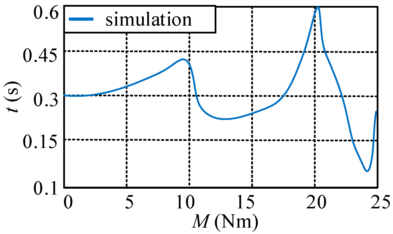
3.3. Driving Force Distribution Analysis

Since the swing arms and main track are driven by the same motor, the robot automatically distributes torque to the swing arms and main track based on operating conditions during adaptive obstacle overcoming. In other words, when the robot overcomes an obstacle with the torque entirely supplied by either the main track or the swing arms, it corresponds to distinct obstacle-overcoming time. Due to the presence of a torque self-distribution mechanism, the actual obstacle-overcoming time lies between these two distinct obstacle-overcoming times. This chapter primarily aims to obtain the range of obstacle-overcoming time for the robot’s obstacle overcoming under different torque drives through numerical calculations.

Furthermore, by assessing how much the time exceeds the minimum duration, one can evaluate the robot’s performance during the adaptive obstacle traversal process. The flowchart illustrating the process of determining the minimum obstacle-overcoming time, and its corresponding torque allocation, is depicted in Figure 9.

According to the geometry of the track and the rocker, the relationship between torque M and force F is as follows:

$$F=\frac{M_0-M}{r\mathrm{Sin}\theta }$$

(28)

Combining Equations (27) and (28), the mathematical programs of the numerical cycle to calculate the time spent on step climbing can be expressed as:

(1)

Solving the differential Equations;

$$\{\begin{array}{c}\theta \left(0\right)=0\\ \frac{d}{dt}\frac{\partial T}{\partial \dot{q}}-\frac{\partial T}{\partial q}=Q\\ \dot{\theta }\left(0\right)=2.5\end{array}$$

(29)

(2)

Obtaining a function of position and time;

$$\begin{array}{c}\theta \left(t\right)=f_1\left(t\right)\\ \dot{\theta }\left(t\right)=f_2\left(t\right)\end{array}$$

(30)

(3)

Obtaining the time when climbing completes;

$$f_1\left(t\right)=\frac{\pi }{2}-\frac{23.25}{180}\pi$$

(31)

(4)

Calculate all the distributions and select the distribution where the time is minimum.

Executing the mathematical program, the relationship between time and torque is expressed as follows.

As shown in Figure 10, it is stated that, when the moment of 25 Nm is entirely distributed to the rocker, the corresponding obstacle-overcoming time is approximately 0.2 s. To further validate the theoretical analysis, we utilized the multi-body dynamics software to conduct a simulated simulation of the robot overcoming a single-step obstacle.

3.4. Simulation of the Process of Obstacle Overcoming

The motion-simulation process of the robot climbing a single step is depicted in Figure 11, which is conducted using the multi-body dynamics software. The virtual prototype of the robot is simulated using a step model with dimensions of 200 mm in height and 250 mm in width.

As shown in Figure 11a, the robot prepares to overcome the obstacle before reaching the step. At this point, the main tracks of the robot and the tracks of the passive swing arms move simultaneously, driving the robot toward the step. When the front end of the passive swing arms contacts the first step, as shown in Figure 11b, the tracks of the passive swing arms stop moving, while the planet carrier, due to its redundant degree of freedom, rotates to a certain angle. When one side of the passive swing arms is fully attached to the vertical surface of the step, as shown in Figure 11c, the robot reaches the critical position for climbing the obstacle. Under the effect of frictional force acting on the main track, the center mass of the robot is raised, as shown in Figure 11d. Then, both passive swing arms successfully climb over the step, as shown in Figure 11e.

Using multi-body dynamics software to establish the dynamic model of the robot and simulate the obstacle-overcoming process, the variation of the angle, angular velocity, and angular acceleration of crankshaft 1 is obtained. These results will be compared and analyzed with the theoretical calculation results presented earlier. Setting M to 25 Nm and time to 0.4 s, the comparison of angle, angular velocity, and angular acceleration curves are shown in Figure 12a–c.

4. Prototype and Experiment

4.1. Design of the Control System

The control system of the robot is mainly divided into four parts: the power-supply unit, the control unit, the perception unit, and the measurement unit. As shown in Figure 13, the power-supply unit is primarily powered by a battery that provides power to the entire robot. It directly supplies power to the motor drive board and signal-receiver terminal. Additionally, a voltage-reduction module is installed to power the Arduino control board. The control unit primarily receives signals from the remote controller through the signal-receiver terminal and then transmits them to the Arduino control board for processing. The processed signals drive the motor drive board, thereby controlling the motors. Furthermore, in order to perceive the working environment in which the robot operates, front and rear cameras are installed. Lastly, to measure the power of the robot under different operating conditions, the measurement unit includes a power-measurement module. The current and voltage data obtained through measurement are transmitted to the computer through the Bluetooth module.

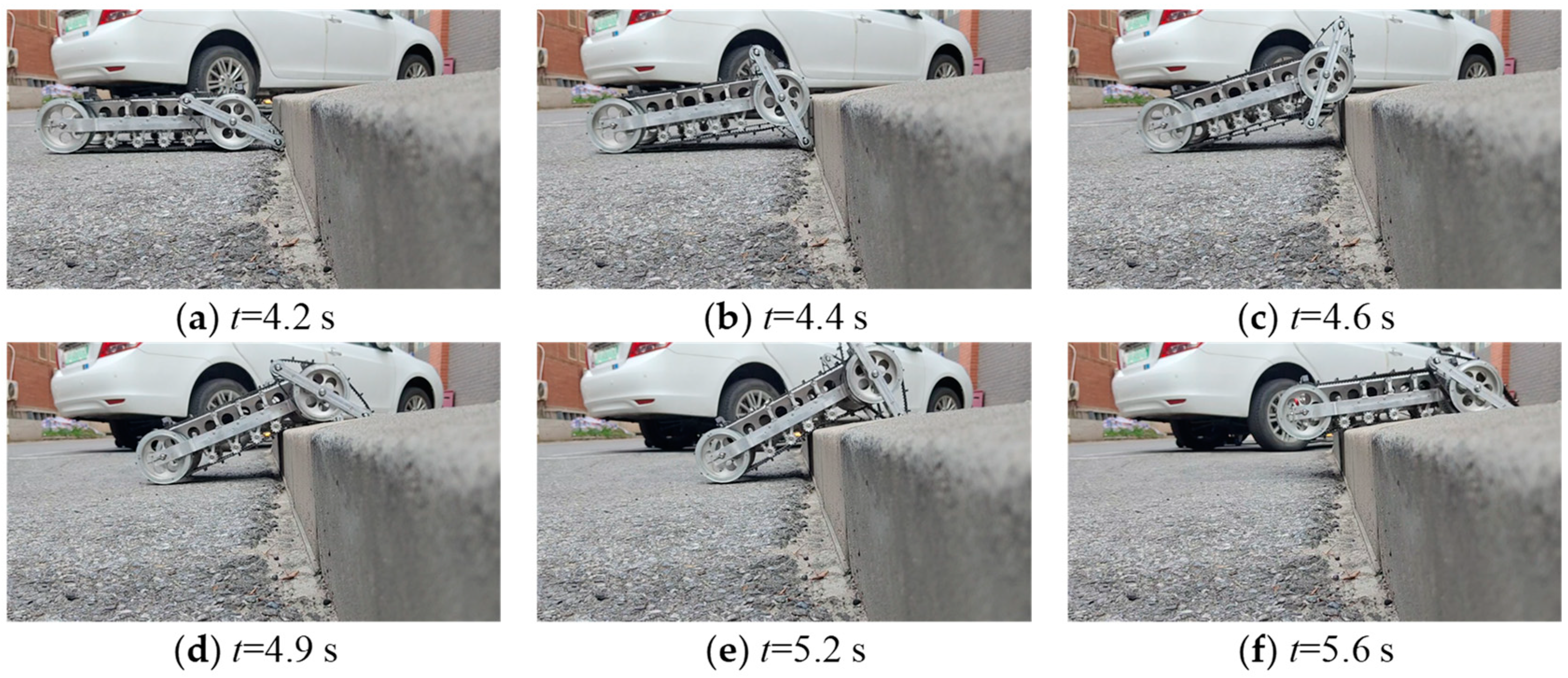
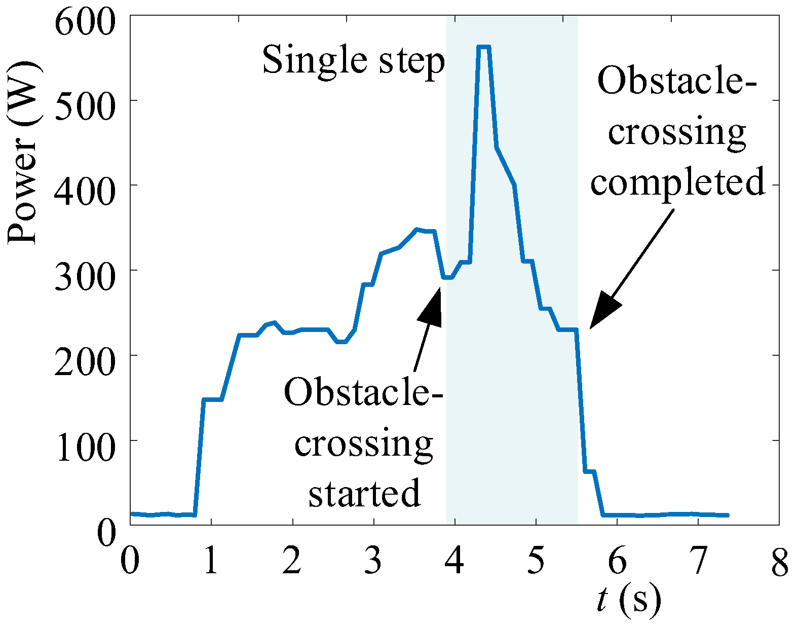
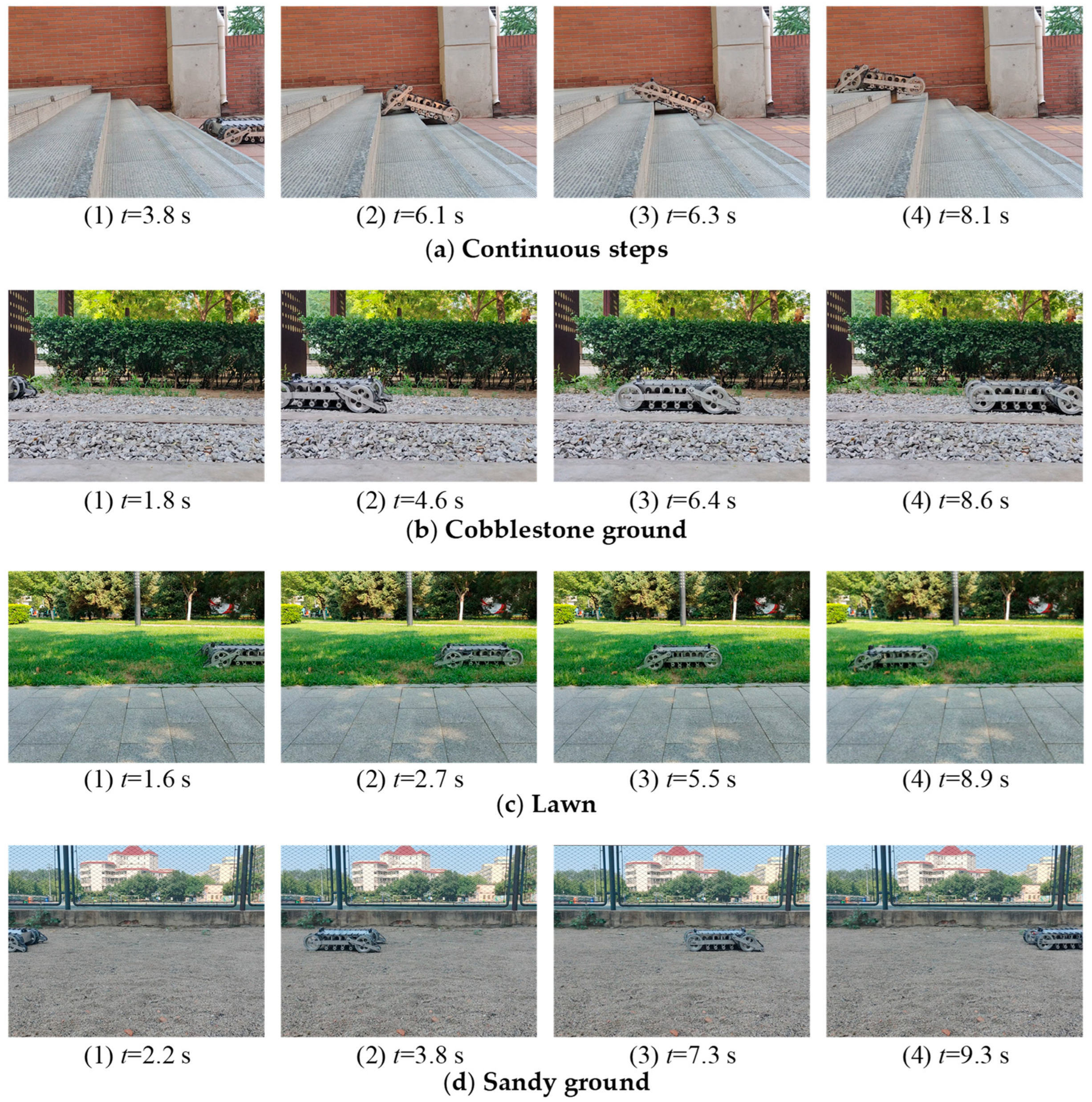
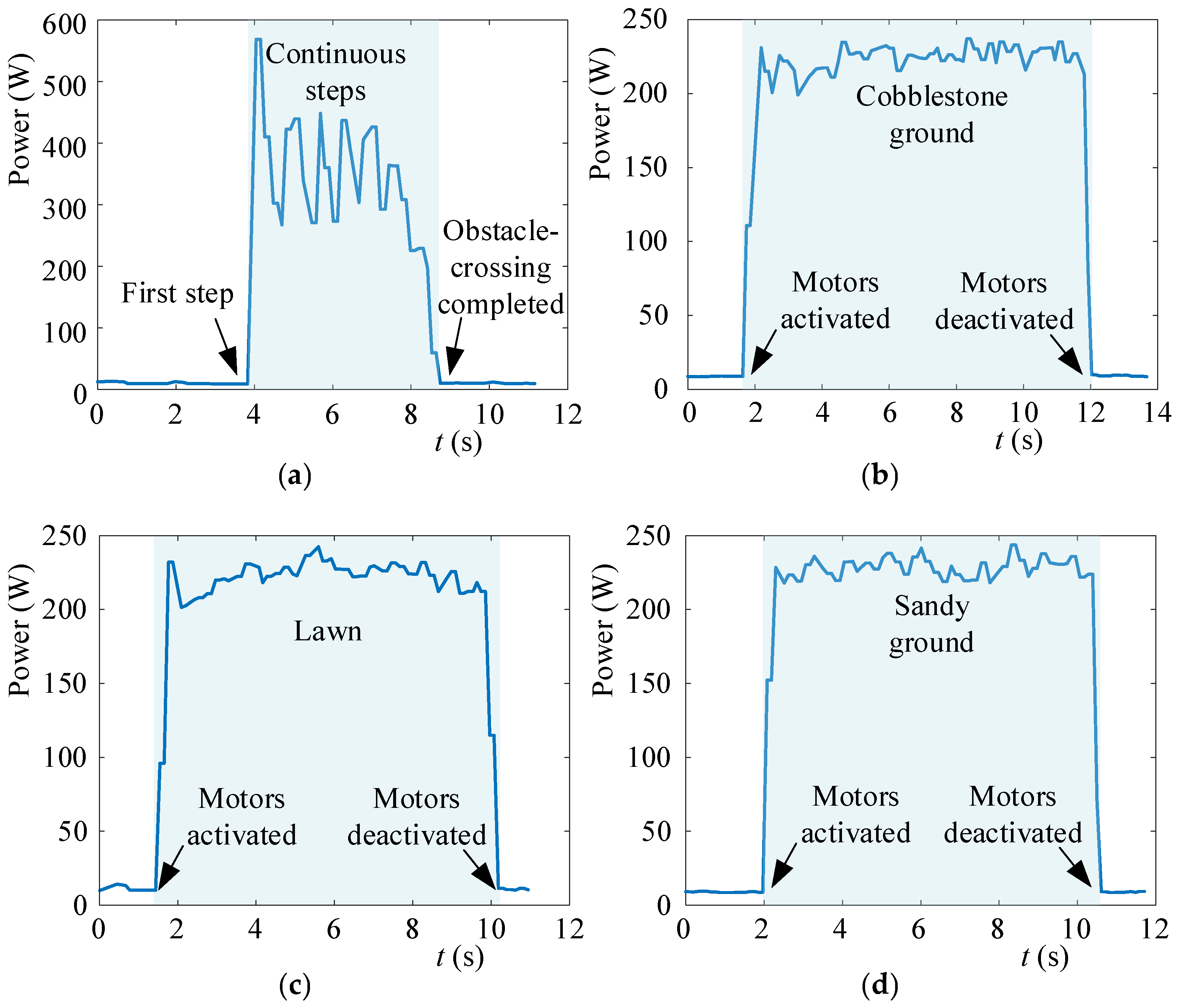
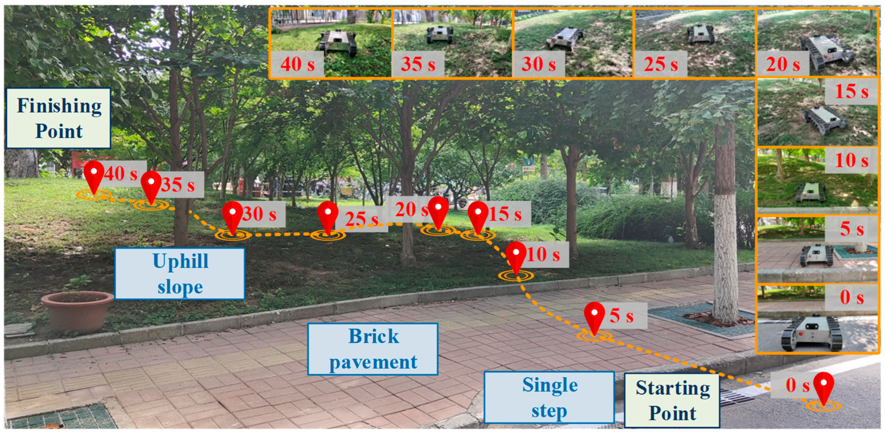
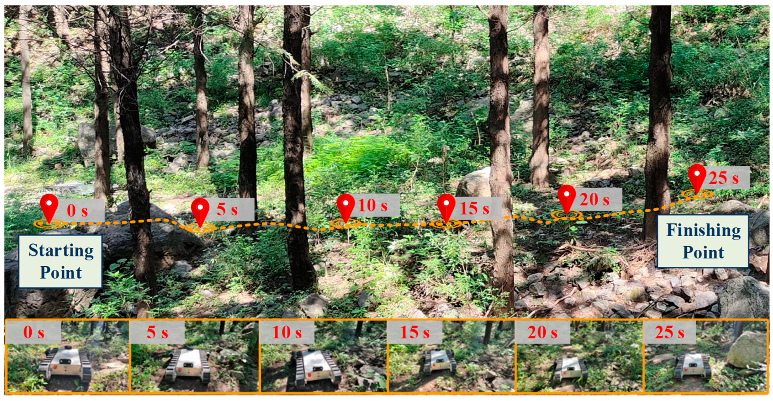
4.2. Experimental Tests

In order to verify the rationality of the robot’s mechanical design and the validity of the kinematic and dynamic analysis, the robot is fabricated and tested to ensure that it can achieve the desired functions. The robot’s shell is made of stainless steel, which can protect the internal components and crucial sensors of the robot when navigating through complex environments. The overall dimensions of the robot are 780 mm × 600 mm × 200 mm, and it weighs 20 kg. The maximum speed of the robot reaches 2 m/s, and other performance parameters are shown in

Table 2. Parameters of the prototype.

Length (mm)	Width (mm)	Height (mm)	Weight (kg)	Number of Motors	Top Speed(m/s)	Surmountable Obstacle Height (mm)
780	600	200	20	2	2	250

.

To verify the theoretical analysis and virtual simulation from Chapter 2 to Chapter 4, we experimented with the robot’s climbing of a single step. The climbing process is illustrated in Figure 14. At 4.2 s, the robot’s swing arms contact with the step (a). After 0.2 s, the robot is lifted (b). By 4.6 s, the robot is completely lifted onto the step (c). Another 0.3 s later, the robot’s front end has climbed onto the step (d). Subsequently, the robot continues to climb upward, assisted by the frictional force between the body and the step (e), and completes the climbing at 5.6 s (f).

As shown in Figure 14, it is worth noting that the time it takes for the robot to transition from state (a) to state (b), i.e., from the flat surface to the lifted position, is approximately 0.2 s, which closely matches the time required for single-step climbing, as predicted in our previous Section 3.3 on torque distribution and 3.4 on dynamic simulations. During the experiment, we measured the power variation of the robot during the climbing of the step, as shown in Figure 15.

After analyzing the robot’s performance in overcoming a single-step obstacle, we conducted tests on its performance in other common environments, as shown in Figure 16. These environments include (a) continuous steps, (b) cobblestone ground, (c) lawn, and (d) sandy ground. We also measured the power consumption of the robot’s movement in these four environments, as shown in Figure 17.

From Figure 16a, it can be observed that, when the robot climbs consecutive steps, the power consumption is highest when climbing the first step, which is roughly equivalent to the power consumption when climbing a single step. However, as the robot continues climbing consecutive steps, the power consumption decreases. This is because after the robot climbs the first step, the width of the step is relatively small, and the robot starts climbing the second step without being fully parallel to the ground. At this point, the robot is still in a tilted position, allowing it to continue climbing consecutively without the need for being lifted again.

After testing the robot in various single environments, we selected a real outdoor environment with multiple complex obstacles to conduct experiments to assess the feasibility of the robot completing complex tasks in the real world. As shown in Figure 18, the selected environment includes four types of obstacles: tarmac (1 m in length), two single steps (0.15 m/0.1 m in height), brick pavement (5 m in length), and grassy uphill (1 m in height). In the experiment, the starting point and finishing point were set, and the robot performed the tasks under remote control by the operator. Initially, the robot set off from the starting point and utilized its passive rocking arms to ascend the first step, which was approximately 0.15 m in height. Subsequently, it traveled about 2 m along a path that had been laid out with turns and surmounted the second step, which was approximately 0.1 m in height. Following the staircase traversal, the robot climbed up a slope adorned with grass, ultimately arriving at the termination point. Snapshots of the task process are shown in Figure 18, and the corresponding videos will be uploaded as attachments. Furthermore, we conducted experiments in the wild forested area, and the relevant details are illustrated in Figure 19.

5. Discussion and Future Works

The main limitation of tracked robots is their limited capability of overcoming high obstacles such as steps. Many scholars achieve obstacle overcoming by adding active swing arms to tracked robots and additional motors. When the robot detects an obstacle, it stops and actively adjusts the pitch angle of the swing arms to climb the obstacle. The tracked robot with passive swing arms in this paper can achieve obstacle crossing by adaptively switching between the rotation mode and the track mode of the swing arms. The robot can drive, steer, and flip over the obstacle by using only two motors.

Through analysis, we can find that the obstacle-overcoming height of this robot mainly depends on the length of the planet carrier and planetary gear of the passive swing arms. Increasing the length of the planet carrier and planetary gear will increase the obstacle-overcoming height of the robot, though the torque required by the robot will also increase. Therefore, in order to design this robot, we should first determine the general obstacle height of the application environment, then determine the length of the planet carrier and planetary gear, and finally determine the motor torque through dynamic analysis and simulation.

For the proposed robot, when it may encounter a small obstacle, the passive swing arms will automatically flip over the obstacle; that is, the passive swing arms are uncontrollable, which is not conducive to the stability of the robot. In order to solve this problem, we plan to add a relay between the main tracked assembly and the passive swing arms. When the robot needs to overcome the obstacles, the relay does not work, and the swing arms can flip freely. When the robot does not need to overcome the obstacles, the relay works so that the passive swing arms are fixed to the main tracked assembly.

At present, the proposed robot has mainly been tested in single scenarios and relatively ideal environments. For more complex practical environments, such as rocky surfaces, we believe that this is complex, and more work needs to be done. In the future, we will first collect the parameters of complex obstacles in the real environment, then establish a model of complex obstacles through simulation software for simulation, and, finally, optimize the structure of the robot to conduct experiments in more complex scenarios.

The proposed robot still requires remote control by an operator to reach its destination currently. In future work, we will enhance the robot’s perception capabilities and develop a 3D path-planning algorithm; by installing sensors and machine-vision cameras, the robot can automatically complete tasks in complex scenarios.

6. Conclusions

This paper presents a novel adaptive obstacle-overcoming tracked robot with two passive swing arms. The ability to overcome obstacles of the presented robot is achieved by creative design through the coupling of the main track and passive swing arms based on the property of the underactuated of the passive swing arms. The mechanical design of the proposed tracked robot is presented, and a kinematic and dynamic analysis of the proposed robot is conducted. Through numerical simulation, the obstacle-overcoming ability of the robot is verified. Further, a physical prototype of the robot is designed and fabricated. Field tests were subsequently carried out to prove the design concept, feasibility, maneuverability, and obstacle-overcoming ability of the proposed robot. The novel tracked robot proposed in this paper provided new insights into the simple design of mobile robots, which have potential applications in the fields of reconnaissance, surveillance, and homeland security in complex terrains.

References

1. Delmerico, J.; Mintchev, S.; Giusti, A.; Gromov, B.; Melo, K.; Horvat, T.; Cadena, C.; Hutter, M.; Ijspeert, A.; Floreano, D.; et al. The Current State and Future Outlook of Rescue Robotics. J. Field Robot. 2019, 36, 1171–1191. [Google Scholar] [CrossRef]
2. Ugenti, A.; Vulpi, F.; Domínguez, R.; Cordes, F.; Milella, A.; Reina, G. On the Role of Feature and Signal Selection for Terrain Learning in Planetary Exploration Robots. J. Field Robot. 2022, 39, 355–370. [Google Scholar] [CrossRef]
3. Milella, A.; Reina, G.; Nielsen, M. A Multi-Sensor Robotic Platform for Ground Mapping and Estimation beyond the Visible Spectrum. Precis. Agric 2019, 20, 423–444. [Google Scholar] [CrossRef]
4. Nakajima, S. Concept of a Novel Four-Wheel-Type Mobile Robot for Rough Terrain, RT-Mover. In Proceedings of the 2009 IEEE/RSJ International Conference on Intelligent Robots and Systems, St. Louis, MO, USA, 10–15 October 2009; pp. 3257–3264. [Google Scholar]
5. Jiang, H.; Xu, G.; Zeng, W.; Gao, F. Design and Kinematic Modeling of a Passively-Actively Transformable Mobile Robot. Mech. Mach. Theory 2019, 142, 103591. [Google Scholar] [CrossRef]
6. Katz, B.; Carlo, J.D.; Kim, S. Mini Cheetah: A Platform for Pushing the Limits of Dynamic Quadruped Control. In Proceedings of the 2019 International Conference on Robotics and Automation (ICRA), Montreal, QC, Canada, 20–24 May 2019; pp. 6295–6301. [Google Scholar]
7. Zi, P.; Xu, K.; Tian, Y.; Ding, X. A Mechanical Adhesive Gripper Inspired by Beetle Claw for a Rock Climbing Robot. Mech. Mach. Theory 2023, 181, 105168. [Google Scholar] [CrossRef]
8. Tang, Z.; Dai, J.S. Bifurcated Configurations and Their Variations of an 8-Bar Linkage Derived from an 8-Kaleidocycle. Mech. Mach. Theory 2018, 121, 745–754. [Google Scholar] [CrossRef]
9. Tang, Z.; Wang, K.; Spyrakos-Papastavridis, E. Origaker: A Novel Multi-Mimicry Quadruped Robot Based on A Metamorphic Mechanism. J. Mech. Robot. 2022, 14, 060907. [Google Scholar] [CrossRef]
10. Yao, S.; Yao, Y.; Liu, R.; Liu, C. A Portable Off-Road Crawling Hexapod Robot. J. Field Robot. 2022, 39, 739–762. [Google Scholar] [CrossRef]
11. Klemm, V.; Morra, A.; Salzmann, C.; Tschopp, F.; Bodie, K.; Gulich, L.; Küng, N.; Mannhart, D.; Pfister, C.; Vierneisel, M.; et al. Ascento: A Two-Wheeled Jumping Robot. In Proceedings of the 2019 International Conference on Robotics and Automation (ICRA), Montreal, QC, Canada, 20–24 May 2019; pp. 7515–7521. [Google Scholar]
12. Bjelonic, M.; Sankar, P.K.; Bellicoso, C.D.; Vallery, H.; Hutter, M. Rolling in the Deep—Hybrid Locomotion for Wheeled-Legged Robots Using Online Trajectory Optimization. IEEE Robot. Autom. Lett. 2020, 5, 3626–3633. [Google Scholar] [CrossRef]
13. Zhang, G.; Ma, S.; Liu, J.; Zeng, X.; Kong, L.; Li, Y. Q-Whex: A Simple and Highly Mobile Quasi-Wheeled Hexapod Robot. J. Field Robot. 2023, 40, 1444–1459. [Google Scholar] [CrossRef]
14. Chen, H.-Y.; Wang, T.-H.; Ho, K.-C.; Ko, C.-Y.; Lin, P.-C.; Lin, P.-C. Development of a Novel Leg-Wheel Module with Fast Transformation and Leaping Capability. Mech. Mach. Theory 2021, 163, 104348. [Google Scholar] [CrossRef]
15. Rubio, F.; Valero, F.; Llopis-Albert, C. A Review of Mobile Robots: Concepts, Methods, Theoretical Framework, and Applications. Int. J. Adv. Robot. Syst. 2019, 16, 2. [Google Scholar] [CrossRef]
16. Bruzzone, L.; Nodehi, S.E.; Fanghella, P. Tracked Locomotion Systems for Ground Mobile Robots: A Review. Machines 2022, 10, 648. [Google Scholar] [CrossRef]
17. Fukuoka, Y.; Oshino, K.; Ibrahim, A.N. Negotiating Uneven Terrain by a Simple Teleoperated Tracked Vehicle with Internally Movable Center of Gravity. Appl. Sci. 2022, 12, 525. [Google Scholar] [CrossRef]
18. Zong, C.; Ji, Z.; Yu, J.; Yu, H. An Angle-Changeable Tracked Robot with Human-Robot Interaction in Unstructured Environments. Assem. Autom. 2020, 40, 565–575. [Google Scholar] [CrossRef]
19. Yamauchi, B.M. PackBot: A Versatile Platform for Military Robotics. In Proceedings of the Unmanned Ground Vehicle Technology VI, Orlando, FL, USA, 2 September 2004; SPIE: Bellingham, WA, USA; Volume 5422, pp. 228–237. [Google Scholar]
20. Han, X.; Lin, M.; Wu, X.; Yang, J. Design of An Articulated-Tracked Mobile Robot with Two Swing Arms. In Proceedings of the 2019 IEEE 4th International Conference on Advanced Robotics and Mechatronics (ICARM), Toyonaka, Japan, 3–5 July 2019; pp. 684–689. [Google Scholar]
21. Wang, W.; Wu, D.; Wang, Q.; Deng, Z.; Du, Z. Stability Analysis of a Tracked Mobile Robot in Climbing Stairs Process. In Proceedings of the 2012 IEEE International Conference on Mechatronics and Automation, Chengdu, China, 5–8 August 2012; pp. 1669–1674. [Google Scholar]
22. Guo, W.; Qiu, J.; Xu, X.; Wu, J. TALBOT: A Track-Leg Transformable Robot. Sensors 2022, 22, 1470. [Google Scholar] [CrossRef] [PubMed]
23. Bruzzone, L.; Baggetta, M.; Nodehi, S.E.; Bilancia, P.; Fanghella, P. Functional Design of a Hybrid Leg-Wheel-Track Ground Mobile Robot. Machines 2021, 9, 10. [Google Scholar] [CrossRef]
24. Nodehi, S.E.; Bruzzone, L.; Fanghella, P. SnakeTrack, A Bio-Inspired, Single Track Mobile Robot with Compliant Vertebral Column for Surveillance and Inspection. In Proceedings of the Advances in Service and Industrial Robotics, Klagenfurt, Austria, 8–10 June 2022; Müller, A., Brandstötter, M., Eds.; Springer International Publishing: Cham, Switzerland, 2022; pp. 513–520. [Google Scholar]
25. Kislassi, T.; Zarrouk, D. A Minimally Actuated Reconfigurable Continuous Track Robot. IEEE Robot. Autom. Lett. 2020, 5, 652–659. [Google Scholar] [CrossRef]
26. Liu, J.; Wang, Y.; Ma, S.; Li, B. Analysis of Stairs-Climbing Ability for a Tracked Reconfigurable Modular Robot. In Proceedings of the IEEE International Safety, Security and Rescue Rototics, Workshop, Kobe, Japan, 6–9 June 2005; pp. 36–41. [Google Scholar]
27. Gong, Z.; Xie, F.; Liu, X.-J.; Shentu, S. Obstacle-Crossing Strategy and Formation Parameters Optimization of a Multi-Tracked-Mobile-Robot System with a Parallel Manipulator. Mech. Mach. Theory 2020, 152, 103919. [Google Scholar] [CrossRef]
28. Lan, G.; Ma, S.; Inoue, K.; Hamamatsu, Y. Development of a Novel Crawler Mechanism with Polymorphic Locomotion. Adv. Robot. 2007, 21, 421–440. [Google Scholar] [CrossRef]
29. Seo, T.; Sitti, M. Tank-Like Module-Based Climbing Robot Using Passive Compliant Joints. IEEE/ASME Trans. Mechatron. 2013, 18, 397–408. [Google Scholar] [CrossRef]
30. Kim, J.; Kim, J.; Lee, D. Mobile Robot with Passively Articulated Driving Tracks for High Terrainability and Maneuverability on Unstructured Rough Terrain: Design, Analysis, and Performance Evaluation. J. Mech. Sci. Technol. 2018, 32, 5389–5400. [Google Scholar] [CrossRef]
31. Kim, J.; Jeong, H.; Lee, D. Performance Optimization of a Passively Articulated Mobile Robot by Minimizing Maximum Required Friction Coefficient on Rough Terrain Driving. Mech. Mach. Theory 2021, 164, 104368. [Google Scholar] [CrossRef]
Figure 1. The composition of the robot.
Machines 11 01051 g001
Figure 2. Schematic diagram of the transmission system.
Machines 11 01051 g002
Figure 3. The composition and principle of passive swing arms: (a) composition and (b) schematic diagram.
Machines 11 01051 g003
Figure 4. Movement modes of passive swing arms: (a) track mode and (b) rotation mode.
Machines 11 01051 g004
Figure 5. Maximum height of the obstacle.
Machines 11 01051 g005
Figure 6. Mesh grids of H with respect to L and r.
Machines 11 01051 g006
Figure 7. The dynamic model of the robot climbing over the single step.
Machines 11 01051 g007
Figure 8. The torque curve of motor (a) where the torque is all provided by the main track and motor (b) where the torque is all provided by the swing arms.
Machines 11 01051 g008
Figure 9. The process of determining the minimum obstacle-overcoming time.
Machines 11 01051 g009
Figure 10. The relationship between time and torque.
Machines 11 01051 g010
Figure 11. Simulation process of the robot climbing a single step.
Machines 11 01051 g011
Figure 12. Dynamic analysis of the robot. Comparison of the numerical calculation and simulation: (a) angle, (b) angle velocity, and (c) angle acceleration.
Machines 11 01051 g012
Figure 13. Hardware composition of the control system.
Machines 11 01051 g013
Figure 14. Process of the robot climbing a single step.
Machines 11 01051 g014
Figure 15. Variational curve of the power in the process of single-step climbing.
Machines 11 01051 g015
Figure 16. Preliminary tests in different scenarios: (a) continuous steps, (b) cobblestone ground, (c) lawn, and (d) sandy ground.
Machines 11 01051 g016
Figure 17. Variational curve of the power of the robot in different scenarios: (a) continuous steps, (b) cobblestone ground, (c) lawn, and (d) sandy ground.
Machines 11 01051 g017
Figure 18. Overview of the outdoor experiment on irregular terrain with illustrations of the robot’s trajectory.
Machines 11 01051 g018
Figure 19. Overview of the outdoor experiment on mountain forest with illustrations of the robot’s trajectory.
Machines 11 01051 g019