Article

Conversion of a Small-Size Passenger Car to Hydrogen Fueling: Simulation of CCV and Evaluation of Cylinder Imbalance

by
Adrian Irimescu
1,*,
Bianca Maria Vaglieco
1,
Simona Silvia Merola
1,
Vasco Zollo
2 and
Raffaele De Marinis
2
1
Science and Technology Institute for Sustainable Energy and Mobility STEMS—CNR, Via G. Marconi 4, 80125 Napoli, Italy
2
Demax SRL, Strada Statale 7 Appia Km 251, 82014 Ceppaloni, Italy
*
Author to whom correspondence should be addressed.
Machines 2023, 11(2), 135; https://doi.org/10.3390/machines11020135
Submission received: 27 December 2022 / Revised: 13 January 2023 / Accepted: 16 January 2023 / Published: 19 January 2023
(This article belongs to the Section Vehicle Engineering)

Abstract

:
In the efforts to achieve zero-emission transportation, hydrogen offers a valid choice as a complete replacement of gasoline. Adapting spark ignition (SI) engines to this alternative fuel can be implemented with relatively minor changes and limited investment in added components. The conversion of a small-size passenger car to hydrogen fueling was evaluated initially from the perspective of achievable range and peak power. Overall, the concept was found to be feasible and comparable to the fully electric version of the vehicle. Cylinder imbalance was found to be one of the possible issues compared to gasoline operation. This study looks in more detail at cycle-to-cycle variability (CCV) and how this could influence vehicle dynamics as well as noise–harshness–vibration (NHV). CCV was simulated with a 0D/1D approach in vehicle-relevant engine speed–load conditions. A dedicated laminar flame speed sub-model was implemented so as to include fuel chemistry effects, while CCV was simulated by inducing perturbations in the initial combustion stages and fuel system characteristics as well as variation of air–fuel ratio throughout flame propagation. Significant improvement of stability was predicted with hydrogen, while cylinder imbalance was found to be one of the main sources of variability. Applying algorithms that compensate for the imbalance through individual injection valve regulation may not be enough to mitigate the identified issue, and more extensive changes of control strategies could be required. The start of injection settings may need to be adapted for each operating condition to maximize the effect of H2 combustion stabilization.

1. Introduction

There are numerous indications that battery electric vehicles will be the dominant propulsion solution for the passenger car sector [1,2]; heavy-duty applications will have a strong hydrogen-powered market share, including internal combustion engines (ICEs) [3]. On the other hand, H2 ICEs could represent a valid choice for small-size passenger cars as well. This allows zero-GHG emissions in a cost-effective manner and has the benefit of seamless integration with the existing maintenance infrastructure.
There is somewhat unanimous consensus that hydrogen will play a major role in energy and transport [4], with power to x through electrolysis to account for a significant share of its production. In the context of green H2, i.e., obtained using renewable energy sources, overall prices will render it competitive with respect to ‘traditional’ fuels [5], even if numerous aspects need to be considered [6,7]. Cost-of-ownership analysis suggests that hydrogen will be cost-competitive with existing energy sources when the infrastructure is ready and by applying the appropriate policies [8]. Within the total cost of ownership, depreciation plays the most important part for passenger cars [9]; this practically means that the investment cost is the greatest financial effort in this category of vehicles, and many owners may consider retrofitting existing combustion-engine-powered cars to use H2. There are several specific aspects that need to be considered, but H2 ICEs will constitute a significant part of the transition towards carbon-free mobility [10]. Dual fueling may represent a valid option for the immediate reduction in ICE carbon footprint [11] with minimal modifications, and when all characteristics are covered (ranging from fuel injection [12], overall control requirements [13], emissions [14,15], boosting-abnormal combustion [16], and even safety [17]) the goal of zero-GHG emissions can be achieved with existing technology and cost-effectively.
The use of hydrogen in spark ignition (SI) engines is relatively straight forward, even if there are several modifications required by the specific properties of this alternative fuel [18]. One of the main drawbacks is that it significantly reduces volumetric efficiency and thus requires means for compensating for lower power density [19]. Improved combustion stability is often cited as an important advantage [20] that enables lean fueling and higher efficiency. On the other hand, the desirable property of high laminar flame speed can result in limitations due to increased pressure rise rates [21]. As previously detailed, while there are multiple aspects that need to be considered when using H2 for powering passenger cars, one reasonable assumption is that overall, the concept is feasible [22], and there is a need for studying specific phenomena in detail so as to ensure the best use of this alternative fuel.
The current work focuses on the cycle-to-cycle variability (CCV) and how this parameter changes when using hydrogen as a complete gasoline replacement in an SI-engine-powered small-size passenger car. Simulations in a 0D/1D framework were performed for several load points representative for urban and highway driving. Compared to previous publications [23,24] the model was updated for simulating variability, and the entire work is focused on the actual application of powering a small-size passenger car. A dedicated CCV sub-model was developed and applied for predicting the effects of H2 on indicated mean effective pressure (IMEP) as well as in-cylinder peak pressure variability. The multi-cylinder architecture of the engine was also taken into account by performing more detailed analysis of the CCV results. Start of injection (SOI) was carefully scrutinized, given its direct influence on air–fuel mixture formation when using H2 (even if only port fuel injection was considered) and its correlation to unwanted phenomena such as backfiring.

2. Materials and Methods

A small-size passenger car was considered for the present study. It is powered by a 600 cc petrol engine that delivers 40 kW peak power. The electric version of the vehicle features a 41 kW electric motor, and the 17.6 kWh battery ensures a 130 km/h top speed and 125–135 km range. An initial evaluation found that the target of 40 kW peak power and around 100 km range could be obtained with H2 fueling [23] by adding a 30 L container alongside the petrol tank. In this way, the vehicle is completely compatible with the current fuel supply chain and would also be prepared for a future zero-emission scenario. Moreover, if the liquid fuel tank is replaced with gas containers, autonomy would increase to over 170 km, which is close to the foreseen maximum distance between H2 refilling stations [25], and ensure a slight margin so as to alleviate range anxiety. Figure 1 shows the overall layout for the studied power unit. Apart from the main control parameters that were included in the model, it also shows the added H2 injectors; it should be noted that the actual location of these metering valves was considered close to the intake valves (i.e., fitted at the end of intake runners). Only the case of port fuel injection was considered, given its easier implementation, with a reduced number of added components.
Table 1 shows the main engine characteristics when fueled with gasoline. Peak power ratings were verified to be reachable with H2 as well [23], with possible limitations of full load characteristics confined only to low rpm [24].

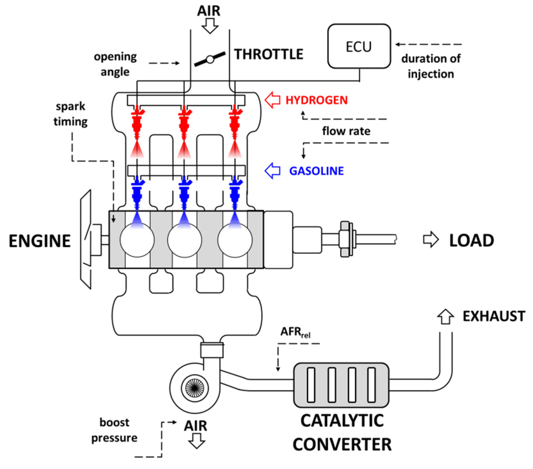
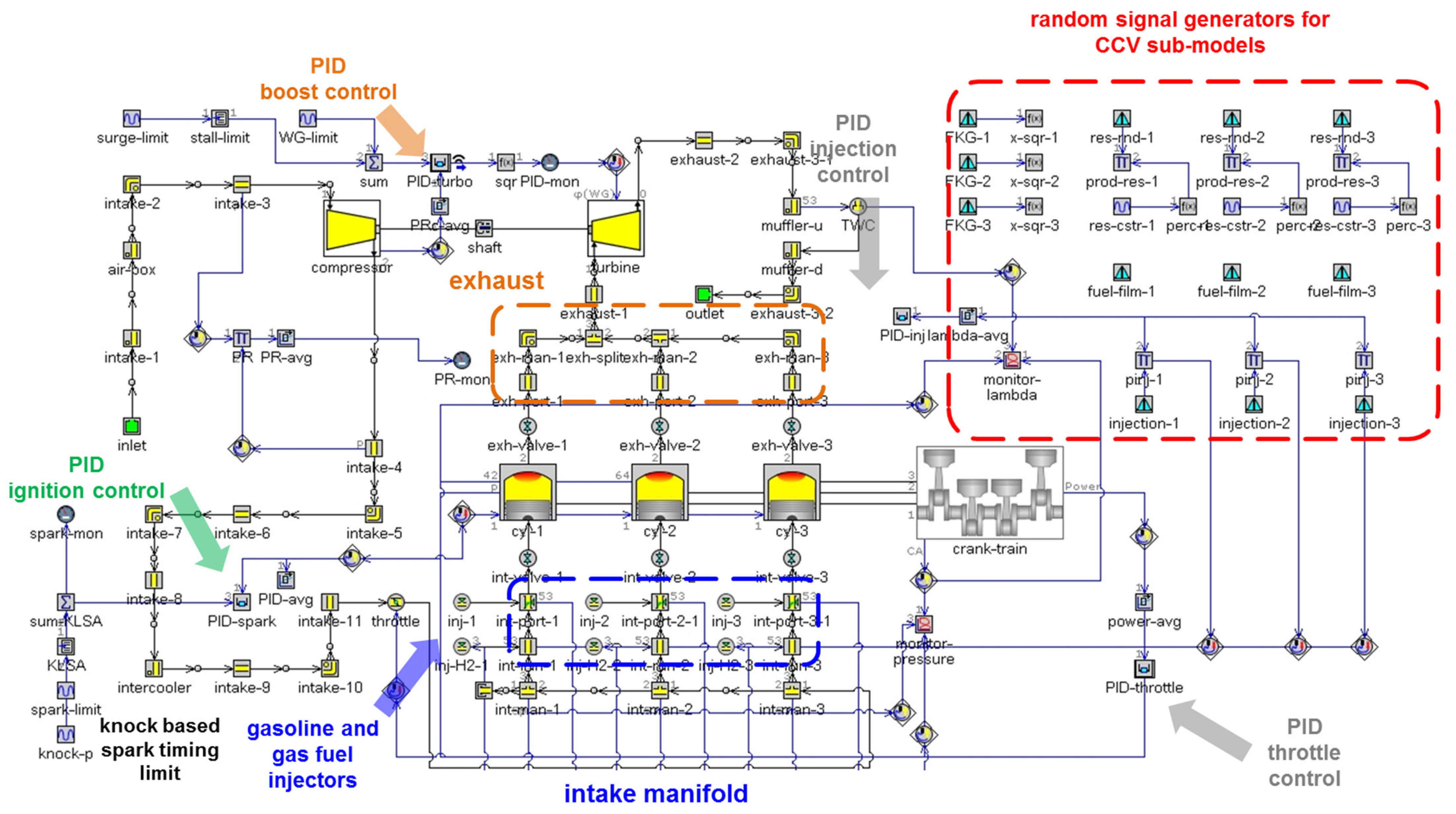
2.1. 0D/1D Model Overview

A disassembled engine was available during the initial phase of model development, and so measurements were performed on several components that were then inserted in the 0D/1D simulation framework [26]. The overall concept is to represent components that feature complex geometries as an equivalent of simple volumes. For example, the intake manifold was implemented as a series of T elements (as shown in Figure 2), the runners were equivalent to round pipes, and so on.
Other OEM data were used for building equivalent turbine and compressor maps [27,28] and for validating (at least partially) model output. More to the point, the simulations predicted peak power with a boost pressure of 0.5 bar, which is completely in line with OEM specifications. Unfortunately, there was no in-cylinder pressure data available for further validation, and so several parameters (e.g., calibration coefficients for the flow and combustion sub-models) were left at their default value.
Previous publications contain more detailed settings of the simulation [23,24], and for brevity, only the specifics of CCV-related sub-models and newly added elements will be described.

2.2. PID Controllers

One issue that was scrutinized was the possible effect of the implemented control components on CCV modeling. More to the point, even after convergence, slight variations of the output signal are always present from one cycle to the next.
The injection PID was implemented in a straightforward manner with a certain target AFR measured in the exhaust line, before the component that models the three-way catalytic converter. The actual engine features two narrow-band oxygen sensors, one before and one after the converter, but only the one upstream is used for controlling injection settings.
Control of engine load was less simple to implement, given that the power unit is turbocharged. For this reason, a certain boost level was set for each load point, and this value represented the target for the PID controller that adjusts the waste gate. The throttle PID was set to achieve a certain power level; for boosted conditions, wide open throttle (WOT) was imposed.
The PID controller that adjusts ignition timing was fed with an MFB50 (i.e., 50% mass fraction burned crank angle point) target of 9 deg aTDC, which was found to be a good compromise of optimized spark control in various conditions [21]. A condition was implemented so as to limit knocking. More to the point, if the model predicted the occurrence of knock, spark timing was reduced by 0.2 deg for the next cycle.
It was found that these three PID controllers induced negligible COV. The boosted condition variability was below 0.1% for IMEP and around 0.3% for peak pressure, mainly due to the fact that knock limitations induced slight variations of the spark timing. These figures were much lower for throttled operation.

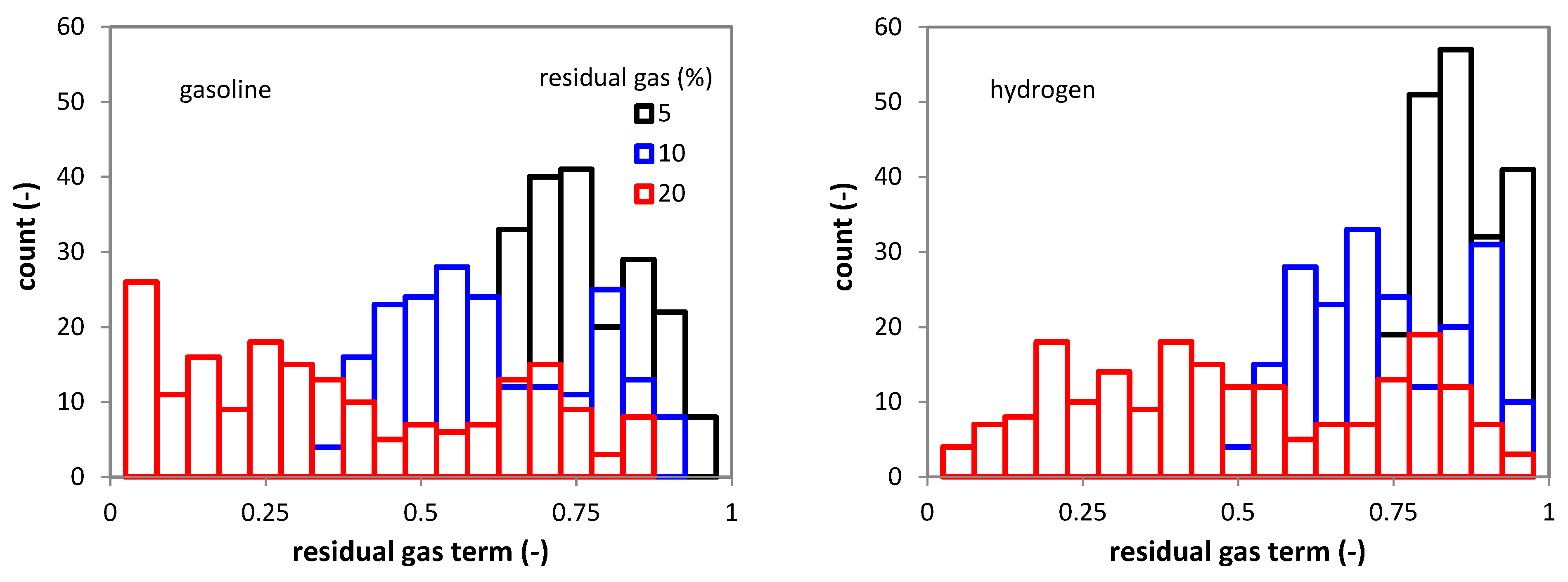
2.3. Cyclic Variability Sub-Model

CCV modeling was approached as in [29], given that it was more fundamentally oriented. The two main assertions were based on the observed correlation of peak pressure variation, due to changes in the duration of the initial stages of combustion, and that of IMEP, mainly due to fluctuations of the injected fuel quantity. The first effect was modeled by implementing a random (uniform distribution) flame kernel growth (FKG) multiplier value for each of the three cylinders. Compared to the previous version of the sub-model, the generation of random numbers was imposed to have a lower limit of 0.794 and an upper limit of 1; the output of the FKG signal generator was then passed to a x10 function, thus resulting in a minimum value of 0.1 and a maximum of 1. Mean values were therefore around 0.897 and 0.337 for the signal generator and FKG, respectively. The additional step allowed the reduction in bias towards larger values of FKG.
The effect related to fuel injection was simply implemented as a random multiplier coefficient between 0.95 and 1.05 applied to the injection duration at the output of the PID controller. This meant that the injected quantity was randomly varied within ±5%, so as to account for pressure pulsation in the fuel rail [30,31]. Variability of the liquid mass added to the fuel film was set between 90 and 100%, given the presence of combined interaction with the port and valves, as well as incoming flow. The imposed figure was based on observed shot-to-shot injection variability, with as high as 7% COV noted in terms of jet penetration in cross-flow conditions [32]. Gas fuel injection is free of fuel film dynamics [33]; therefore, only the pressure pulsations in the rail were kept when performing simulations with H2.
In a first attempt, the model predicted quite low COV for peak pressure at low load. For this reason, it was inferred that the effect of local variation of residual gas concentration (xr) was not accounted for. The basis for this thinking is that when reducing engine load, xr was the main factor of variation in terms of influences within the combustion sub-model. Local residual gas concentration is not distributed uniformly, i.e., even if overall the concentration of diluents is the same from one cycle to the next, the fact that there is a certain degree of stratification will result in different influences on flame propagation and therefore combustion. Measurements in the region of the spark plug have indeed shown that there can be significant local variations of fluid composition from one cycle to the next [34]. Starting from this fundamental observation, a random (uniform distribution) perturbation to the dilution exponent multiplier (DEM) was implemented, thus directly acting on the calculated value of laminar flame speed. A lower limit of 0.1 was imposed, while the upper limit was set at 2.1. The two limits were chosen by considering the effect of dilution on calculated laminar flame speed values, as evidenced in Equations (1) and (2),
S L = [ B m + B Φ · ( Φ Φ m ) 2 ] · ( T u T r e f ) α · ( p p r e f ) β · f ( x r )
f ( x r ) = 1 2.06 · ( x r ) 0.77 · D E M
where SL is the laminar flame speed in m/s, Bm the maximum speed value, BΦ is the roll-off value in m/s, Φ is the equivalence ratio, while Φm is the value at maximum speed, Tu and Tref are the unburned mixture temperature and reference value in K, α and β are the temperature and pressure exponents, p and pref are in-cylinder and reference pressure measured in Pa, while the term f(xr) is used for modeling the effect of residual gas at a mass concentration xr. Full-load conditions usually feature xr values below 5% and consequent reduction of less than 10% of SL (with DEM set at its default value of unity). For part load instead, xr can be as high as 20%, resulting in laminar flame speed values close to 60% lower with respect to the xr = 0 situation. Given the hypothesis of uneven distribution of residual gas, even higher local concentrations are possible; as an example, xr of over 35% would result in over 90% reduction in SL at reference conditions.
Actual implementation of the variations for the DEM was achieved by solving an exponential equation, i.e., by setting the condition f(random · xr) = f(xr), resulting in the formula DEM = ln(random · xr)/ln(xr). For example, with an average xr value of 10%, SL is reduced by around 35%; the lower limit of the random number signal (0.1) would result in close to 6% reduction, while the upper limit (2.1) reduces SL by over 60%. This gives an idea of the variations that were present during the simulations with gasoline. Implementing the influence for the H2 cases was not as straightforward. The residual gas term has a different formula [35,36], and the condition becomes f(random · xr) = 1 − (2.715 – 0.5 · Φ) · random · xr = 1 − 2.06 · xr 0.77 · DEM, thus resulting in a more complex form for calculating the required parameter DEM = ln((2.715–0.5 · Φ) · random · xr/2.06)/(0.77 · ln(xr)). Both calculations were implemented as RLTDependenceXY components, where DEM takes the value calculated by using the derived expression each simulated cycle.
Figure 3 shows the distribution of f(xr) values obtained starting with the same set of 200 random numbers, when changing the residual gas fraction from 5 to 10 and 20%. Evidently, a higher percentage of residual gas results in more consistent reduction in laminar flame speed (low values of function f). It is interesting to note that for both fuels, a wider distribution is predicted at an increasing concentration of residuals. Another important observation is that the effect is different for H2 compared to gasoline; the effect would seem to be less significant for the gaseous fuel, especially at low values of xr.
Overall, with this approach, the model was found to ensure the expected trend when reducing engine load, similar to those usually observed in the literature, e.g., [37].

3. Results and Discussion

Once the model was set up with its sub-components aimed at CCV simulations, several situations were investigated so as to give a better idea on how the engine would perform when fueled with H2 and whether it would significantly influence vehicle dynamics. To this end, the characteristics of the small-size passenger car were used for defining specific operating points. A simple calculation of the power required to drive the car at top speed results in around 31 kW brake power. An overall transmission efficiency of 84% (intended as the ratio between wheel/crankshaft power) was obtained by performing a simplified wheel power requirement calculation at the top speed of 135 km/h. It was assumed that the sixth gear was selected (the gearbox features overall transmission ratios of 14.2, 10.3, 7.4, 5.6, 4.1, and 2.9, respectively), that the vehicle is equipped with a 15-inch rim with 175/55 R15 tire combination; these are equivalent to an engine speed of 4400 rpm and full-load power of 37 kW for a frontal area of 2.4 m2 and a Cx value of 0.37. The aforementioned value of 0.84 is completely comparable to measurements on other vehicles [38]. Using this efficiency figure, four load points were defined at 30, 50, 90, and 130 km/h, chosen as representative of urban and highway driving. This results in a combination of 1.3 kW at 2480 rpm, 3.2 kW at 3130 rpm, 12.5 kW at 2940 rpm, and 33.2 kW at 4240 rpm, respectively, for the four vehicle velocity conditions. Rather than going into a detailed analysis of conversion efficiency (previous publications already give an idea of the relative changes with respect to gasoline [23,24], and more consistent improvements can only be achieved with significant hardware modifications [10]) or emissions (the stoichiometric operation considered throughout the study ensures significant reduction in NOx with a three-way catalytic converter [22]), the results focus on the effects of hydrogen on combustion variability. After an initial evaluation of CCV effects on in-cylinder pressure for the two fuel types, an overview is given of the intended vehicle use. Finally, the effect of SOI was scrutinized as well.

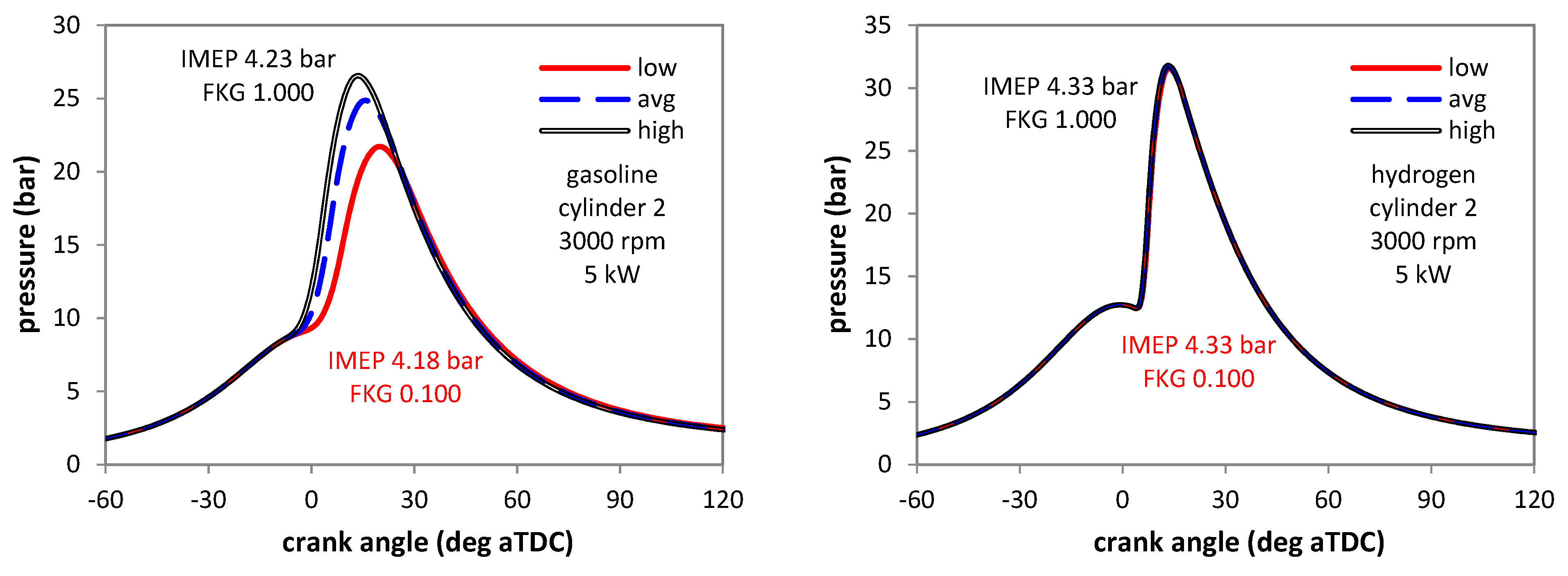
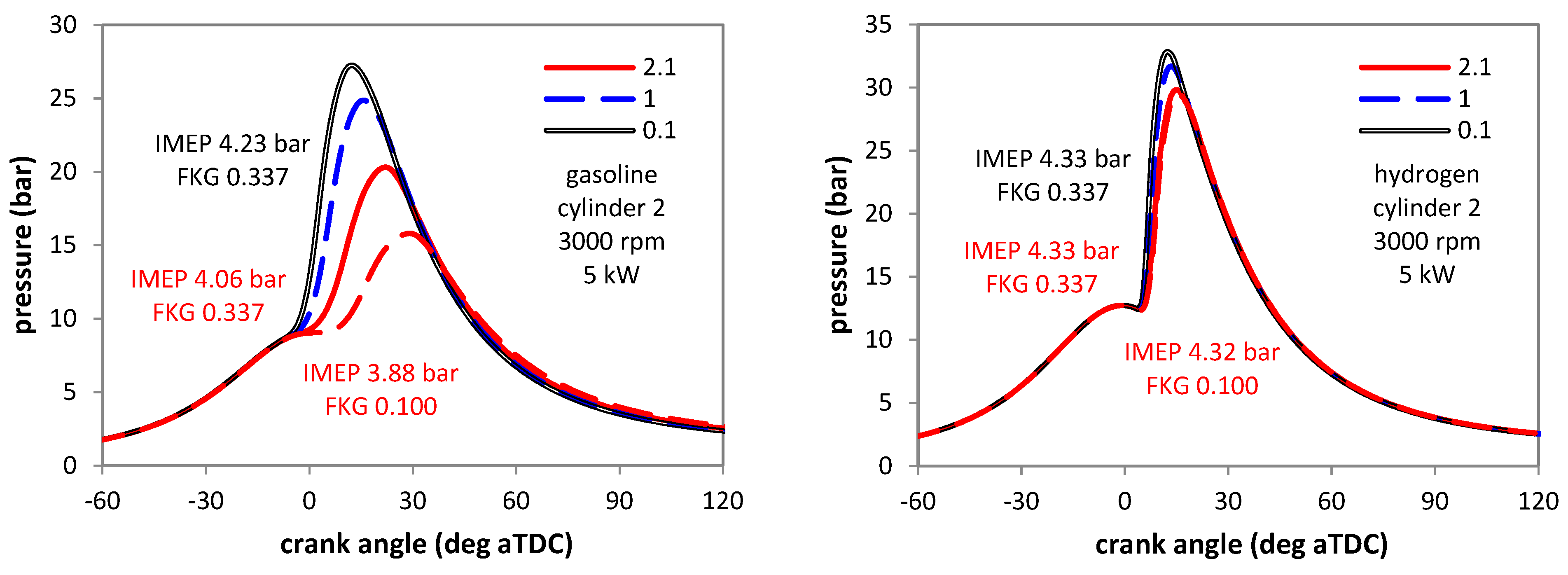
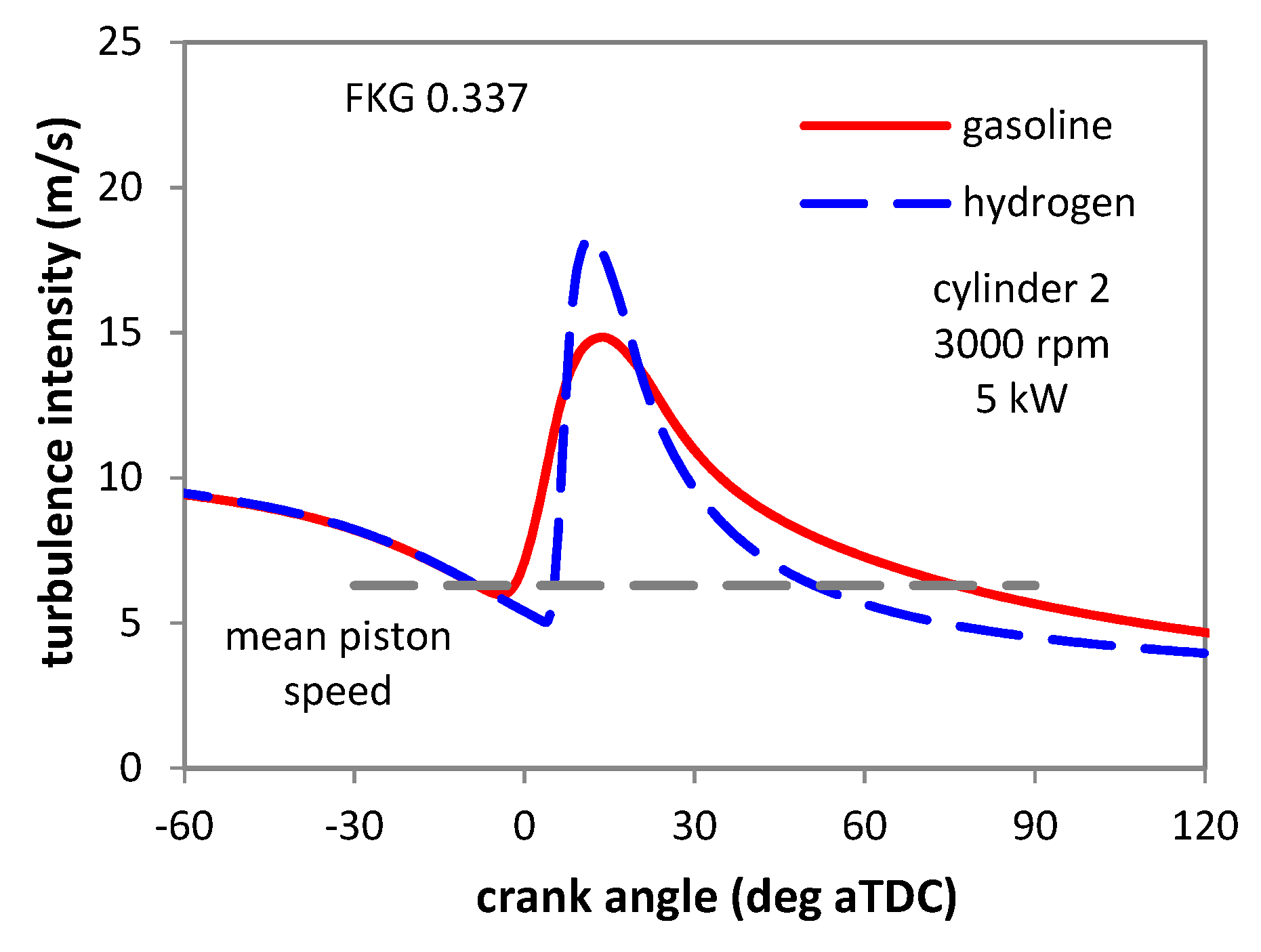
3.1. CCV Effects on In-Cylinder Pressure

A condition of 3000 rpm and 5 kW brake power was arbitrarily chosen for these simulations. Throttled operation was predicted for both fuel types. After an initial step in which the PID controllers were active, the waste gate opening, throttle angle, injection duration, and spark timing were identified for stable operation with the mean FKG and no fuel injection effects. Afterwards, simulations were performed with the fixed control parameters and changing FKG, injection duration, and DEM within the limits imposed in the CCV sub-models. This was done so as to easily identify the effect of induced variability. Figure 4 illustrates the effect of varying the FKG parameter on in-cylinder pressure. A clear difference between gasoline and hydrogen is evident. If, for the liquid fuel, the change resulted in peak pressure variations of up to 5 bar, for H2, the variation was slightly over 0.2 bar. This is directly correlated to the laminar flame speed of the gaseous fuel, predicted to be in the range of 15–20 m/s during combustion (compared to 1.0–1.2 m/s for gasoline); an interesting observation is that it is even higher than the turbulence intensity, calculated to be between 5 and 18 m/s. Therefore, flame propagation is dominated by the laminar process, and the variations during the initial combustion stages are no longer as dominant. The code features a multiplication term in the equation for calculating turbulent flame speed in the form of (1 − 1/(1 + FKG · (Rf/Li)2)), where Rf is the flame radius and Li the integral length scale; this simulates the transition from the laminar flame phase to the turbulent stage. Basically, when the flame radius is 0, the contribution of turbulence is not present, while at large Rf values, the flame is fully turbulent. Evidently, for low FKG, the passage is delayed (resulting in slow flame propagation), while the opposite is true for high FKG figures. The effect of this term is practically insignificant for H2, due to its high laminar flame speed.
As expected, no significant influence on IMEP was simulated. Please note that the results are shown only for cylinder 2; there is a cylinder-to-cylinder difference in volumetric efficiency between the two fuel types, and these effects will be discussed in the ensuing section. Nonetheless, what is immediately evident is that changes in the initial stages of combustion induce slight variations in IMEP for gasoline, while for H2 there was practically no influence.
Figure 5 shows the influence of changing the DEM parameter for the two fuels. Just as for FKG, the effect is much more prominent for gasoline. Even more so, by combining the effect of DEM and FKG (i.e., the ‘worst’ possible situation, characterized by ‘slow’ transition to the turbulent phase and high concentration of residual gas), the code predicts a significant drop in peak pressure as well as IMEP. For hydrogen on the other hand, the influence was much more contained, even if more evident compared to that of changing FKG.
More insight can be gained by analyzing the two parameters that define flame propagation and fuel oxidation in the reaction zone. These are governed by turbulence intensity, its characteristic length, and of course, laminar flame speed.
Figure 6 shows that predicted overall turbulence intensity was quite similar for both fuels; integral length scale was also practically the same. Therefore, the turbulence component in the process of flame propagation should be relatively the same. Laminar flame speed, on the other hand, is over an order of magnitude higher for H2 at reference conditions. As Figure 7 shows, this results in SL values in the range of 10–25 m/s, compared to 0.4–1.6. Apart from the wider range in terms of relative values (around 3–4 times from minimum to maximum DEM during combustion for gasoline, compared to around 2 for H2), the fact that the absolute SL is significantly lower for the liquid fuel means that the influence on in-cylinder pressure is much more pronounced in terms of overall combustion duration. On the contrary, for the gaseous fuel, overall ‘fast’ combustion means that there is less influence of the chemistry part of the process. As detailed in a previous study [21], there is a certain laminar flame speed threshold above which the actual influence on combustion is no longer as evident. Of course, other phenomena such as increased heat loss may result in unwanted effects such as local hotspots, but in terms of an actual link to the thermodynamics of the process, there is less evidence of a connection.

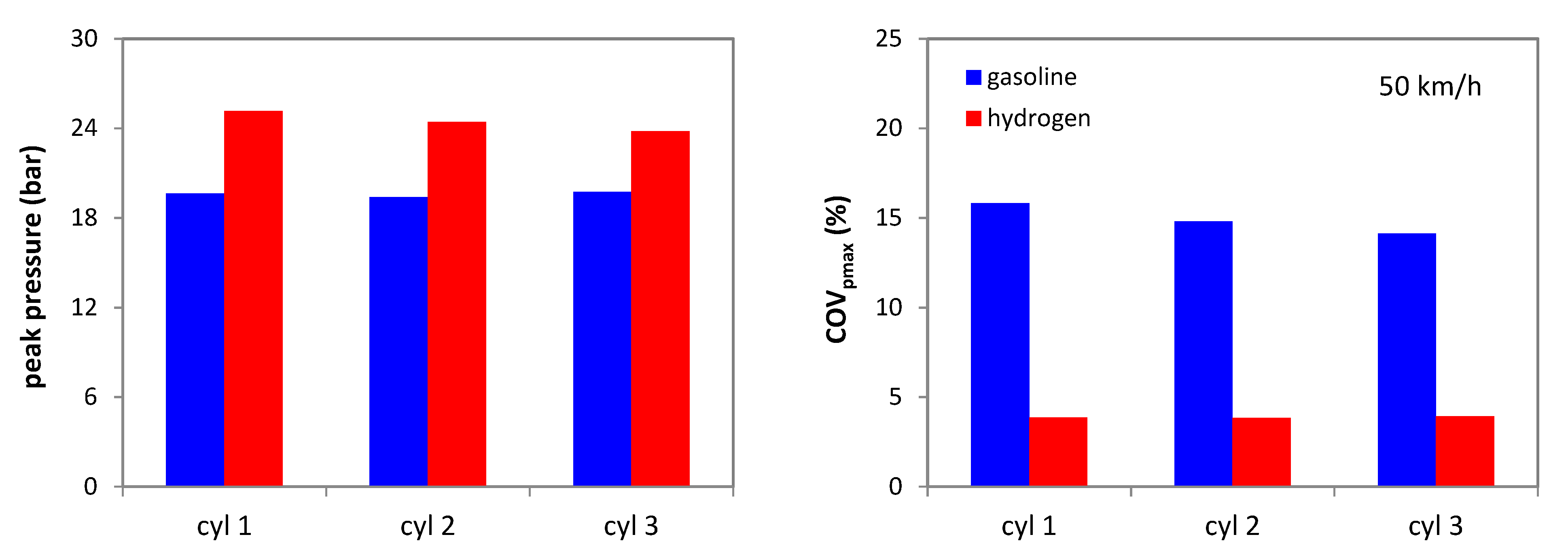
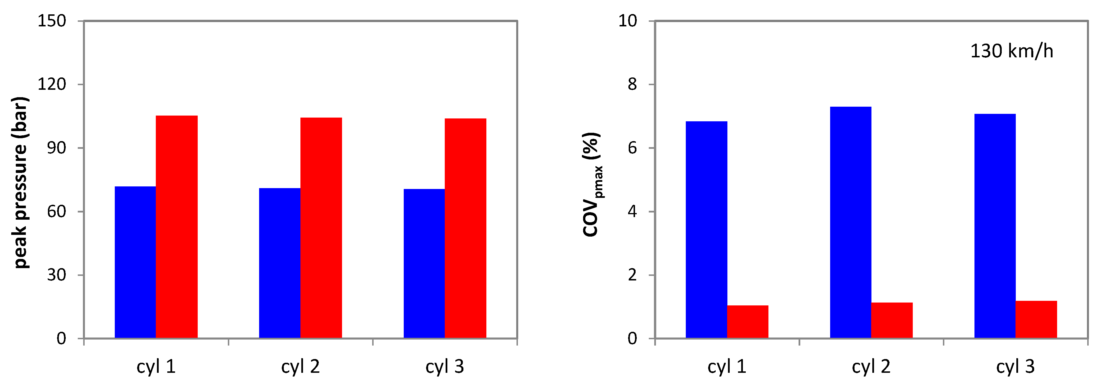
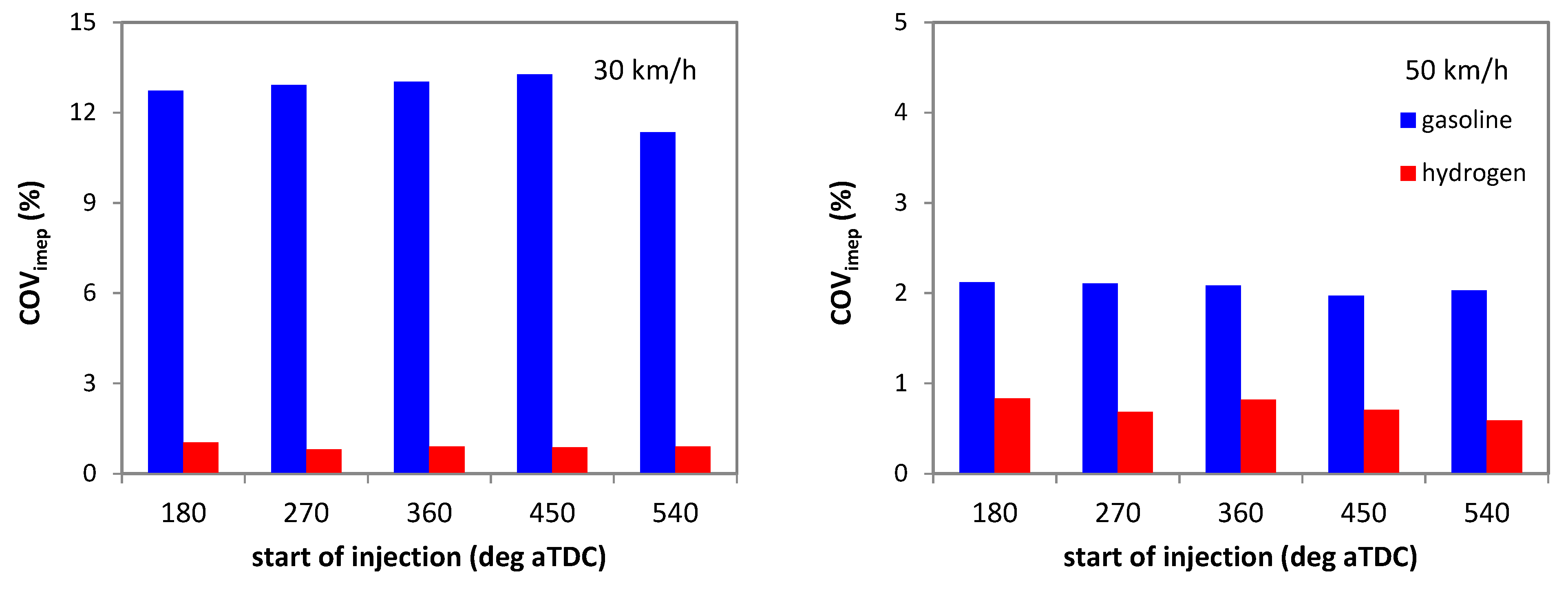
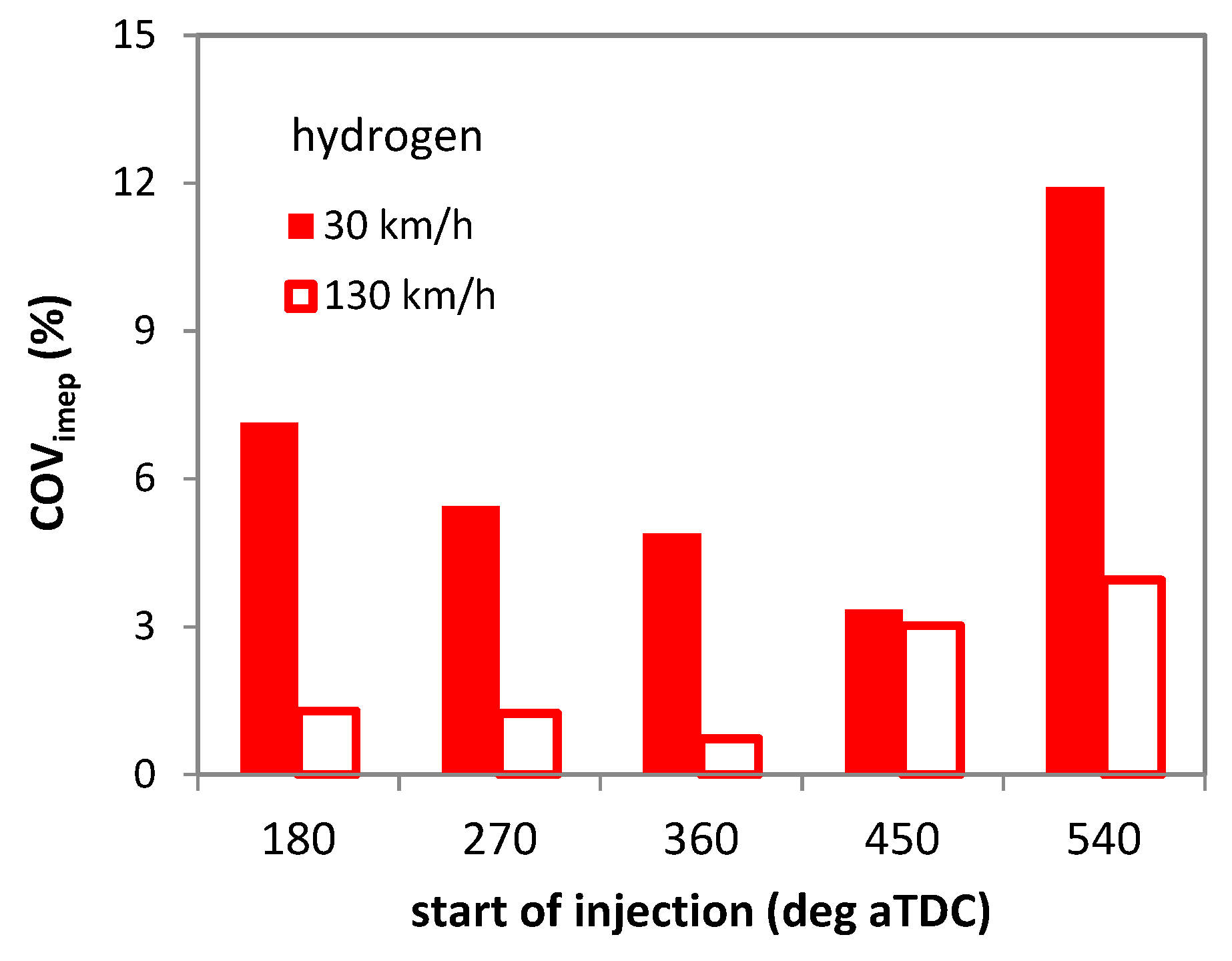
3.2. CCV Effects for Different Vehicle Speed Values

Once the detailed analysis of underlying phenomena was performed for a single operating point, a more comprehensive view was ensured by looking at global parameters and their variability. More to the point, for the actual intended application, the IMEP and its coefficient of variation (COV) are the two essential figures that define usability; the first gives a direct measure of power available to drive the car, and the second can be used for evaluating acceptable noise–harshness–vibration (NVH) limits.
Figure 8 shows the IMEP and COVimep predicted in conditions of constant driving speed at 30, 50, 90, and 130 km/h. The power output was practically the same for both fuels (slight differences, below 1%, were due to the various stable conditions reached by the PID controllers for each operating point), while predicted variability was quite different. For the 30 km/h case, the model predicted a COVimep of over 12% for gasoline, close to the 10% limit considered as the threshold for acceptable engine output variability in automotive applications [39]; of course, continuous driving at 30 km/h is seldom encountered, as at such low speed, start/stop vehicle use due to traffic is more likely. As the engine load increases, less residual gas is present in the cylinder; thus, the related variability is less evident. For 130 km/h, the predicted COVimep was around 1.0% for the liquid fuel and 0.4% for H2. The absolute values are completely comparable to those recorded at similar load on an automotive SI engine [40], and the relative difference between the two fuels is also directly analogous. These results give further confidence to the analysis in terms of the capability of predicting the effects of hydrogen on CCV.
The overall conclusion that can be drawn from the COVimep simulations is that H2 considerably improves stability compared to gasoline, especially in part-load conditions. This hints towards the possibility of operating the engine ultra-lean at low load, thus ensuring important margins for improving efficiency.
The results shown in Figure 8 are crank-train based evaluations, meaning that the COVimep parameter was taken from the “crank-train” component illustrated in Figure 2. This, however, may not be representative for all three cylinders. For this reason, a more detailed analysis was performed at 50 and 130 km/h. Figure 9 shows the predicted IMEP and COVimep for all three cylinders.
If, for gasoline, the cylinder-to-cylinder IMEP variation was below 1% at 50 km/h, with H2, this parameter was close to 4%; at 30 km/h, the difference was even more prominent, at over 10%. Somewhat counter-intuitively, the situation was the opposite for the 130 km/h case, for which gasoline featured the higher figure. This further highlights particular aspects that would normally be neglected (e.g., with gasoline fueling) but that may become important with H2. Cylinder imbalance was indeed identified as a possible issue [23] which results in different volumetric efficiency for each cylinder. Even if this parameter was overall around 26.5% for the 50 km/h case, the individual volumetric efficiency was 25.7, 26.3, and 27.5% for cylinders 1, 2, and 3, respectively; this is the main reason for the predicted relative air–fuel ratios of 0.91, 0.97, and 1.09 at cycle start (exhaust lambda was instead close to stoichiometric). As a consequence, the COVimep of cylinder 3 was more than twice that of the other two cylinders. Interestingly enough, the situation is not exactly the same for the 130 km/h case, for which cylinder 2 featured the highest variability when using hydrogen.
No direct correlation to volumetric efficiency (and therefore lambda values) of each cylinder can be made with respect to COV, but it is one of the main factors of influence. More to the point, even if the combustion CCV model is linked primarily to residual gas concentration at ignition and not volumetric efficiency, the fact that there are larger differences in cylinder-to-cylinder filling performance results in more pronounced effects of this phenomenon on variability. In fact, as Figure 10 shows, much higher COV values are obtained when performing the analysis based on cylinder-to-cylinder data rather than the crank-train component. For completeness, the results shown in Figure 8 were obtained by considering IMEP during the last 200 cycles of the simulation (which totaled 3000 cycles for each point) recorded in the crank-train component, while those shown in Figure 10 were the product of considering a dataset of all three cylinders during the last 200 cycles of the simulation (thus a population three times larger compared to the previous evaluation). Nonetheless, all COV values were significantly lower for the gaseous fuel compared to gasoline.
One other reason for concern is that peak pressure tends to be higher when using hydrogen. The main reason is its ‘faster’ combustion; lower volumetric efficiency requires higher boost levels and thus further contributes to an increase in peak pressure. If at low load this is not a problem (e.g., an increase from around 20 to 25 bar at 50 km/h), at high load this could become an issue. As shown in Figure 11, at 130 km/h, predicted peak pressure was around 70 bar when using gasoline, while with H2 it was over 100 bar. This increase of close to 50% could push the operating regime beyond the limit usually employed for containing peak pressure during the working cycle. Just as for the IMEP data, COVpmax was much lower for the gaseous fuel. The fact that hydrogen features such high laminar flame speed practically eliminates the influence of the FKG parameter and thus greatly reduces variability.
Peak pressure and its variability directly influence knocking and how it is mitigated. Figure 12 shows the maximum pressure predicted for cylinder 2 during the last 200 cycles of the simulation, as well as the calculated knock induction time integral (a value below unity means that no knocking was predicted, while greater than or equal to 1 means that knocking occurs). There is an evident correlation of knocking cycles (those that feature an induction time integral greater than or equal to 1) and peak pressure in the case of gasoline fueling; no abnormal combustion was predicted for hydrogen, given the high RON number of 130 used in the simulations. As mentioned in the previous section, the ignition PID controller contains a limit aimed at preventing knock. Indeed, every time the code would calculate an induction time integral over 1, spark timing would be reduced so as to run the engine at the limit of abnormal combustion. Of course, given the variable nature of combustion, there are cycles that go over the limit, but overall severe knock can be avoided. This poses an interesting question with respect to reduced COVpmax obtained with H2. Even if knocking would occur when using the gaseous fuel, its much more repeatable combustion process could provide the basis for ‘tighter’ control of ignition and thus obtain important gains in efficiency.
As an overall conclusion of the analysis performed in this sub-section, it can be stated that the use of H2 results in significantly lower COV with respect to gasoline. Cylinder imbalance was identified as a possible issue that results in quite a different air–fuel ratio for each individual cylinder. Normally, correction algorithms are developed for handling differences in the range of ±5% [39]; they usually employ an analysis of the signal given by the exhaust gas oxygen sensor to identify deviations from stoichiometry and apply injection trimming to reduce imbalance [41,42,43]. The fact that with H2 fueling the engine features more than double the expected cylinder-to-cylinder difference could be a problem that may result in undesired effects.

3.3. Start of Injection Effects

All the results presented in the previous sub-sections were obtained with a fixed SOI of 360 deg bTDC. This setting was found to be compatible with a wide range of engine speed conditions [24]; intuitively completing the entire fuel delivery process during the intake stroke should minimize the difference in volumetric efficiency from one cylinder to the next, as well as the risk of backfire. In fact, the flow rate of the H2 injectors was imposed at 6 kg/h, which is relatively high for such a small engine size, so as to ensure complete delivery of the fuel required for rated power within a 180 deg window.
Figure 13 shows the results obtained by setting the SOI at during the exhaust stroke (180 and 270 deg aTDC), during intake (360 and 450 deg aTDC), and with the valves closed (540 deg aTDC). It should be noted that all cases featured practically the same IMEP, ensured by the load control through throttling or turbocharging. The fact that not all cases featured the same COV trend when sweeping the SOI highlights the complexity of interactions and further emphasizes the need to carefully evaluate control strategies when considering conversion to H2 fueling. Nonetheless, SOI variations resulted in relatively reduced benefits in terms of COVimep. Low-velocity conditions featured variability much lower than that predicted for gasoline. Only one condition resulted in COVimep higher for H2 (the 90 km/h case with SOI at 450 deg aTDC), but this was directly comparable to the value calculated for the liquid fuel. Therefore, as an overall conclusion, it can be stated that changes in the SOI bring relatively reduced benefits in terms of improving stability. These results were, however, obtained by evaluating crank-train-based IMEP. Given that cylinder imbalance was found to exert an important influence on variability (Figure 10 compared to Figure 8), cylinder-based COV was also scrutinized.
Figure 14 shows the results obtained by extending the population of IMEP values to all three cylinders. While the overall trend is very much the same as that shown in Figure 13 (with SOI360 ensuring a good compromise for all vehicle speed cases), the higher values emphasize the effect of injection phasing on COVimep. One interesting result is that for 30 km/h cruising speed, the model predicted better stability with SOI at 450 deg aTDC. Given the reduced injection duration (below 1 ms), fuel delivery is completed during the intake stroke, even with relatively retarded SOI. For 130 km/h, the best choice was predicted to be SOI 360 deg aTDC; the end of injection was before intake valve closure (IVC) for this case as well (injection duration was slightly below 5 ms).
One other important aspect to be considered is the risk of backfire. The previous study [24] showed the requirements of adjusting SOI settings so as to reduce the risk of fresh charge ignition in the intake port. Basically, the main mechanism is that the H2-air mixture can ignite at intake valve opening (IVO) as it comes in contact with hot residual gas or high-temperature surfaces (e.g., the spark plug or exhaust valve). Minimizing the concentration of fuel at the instant of valve opening would therefore greatly reduce the risk of backfire.
The predicted relative air–fuel ratios in this component at IVO for the 130 km/h case with SOI360 were 2.2, 2.5, and 2.4 for cylinders 1, 2, and 3, respectively. These values were even higher with SOI270, at 3.5, 4.3, and 4.6. When comparing these figures with the explosion limit AFRrel of around 1.8, both SOI settings would feature reduced risk of abnormal combustion. Even if all concentrations are above the lower flammability limit (with an AFRrel of over 9), increasing the lambda value means that backfiring is less likely to occur.
One cause for concern is that the model predicted lambda values of 0.7, 0.9, and 1.0 for cylinders 1, 2, and 3 at 30 km/h with SOI450 (which featured the lowest COVimep). Given that all three cylinders would be at high risk of backfire, this SOI setting would be best avoided. Starting the injection at 360 deg aTDC would bring the AFRrel values to 1.6, 2.0, and 2.4 respectively. Even if cylinder 1 is still below the lambda 1.8 limit, the risk would be greatly reduced compared to the SOI450 setting. The fact that this condition features very low pressure (intake and in-cylinder) as well as high residual gas concentration (around 17% for all three cylinders) further reduces the likelihood of backfire.

4. Conclusions

Within the context of a future zero-GHG emissions scenario, hydrogen fueling of a small-size passenger car was investigated. The overall idea is to achieve complete integration within this scenario of a retrofitted ICE vehicle for ensuring the use of this alternative fuel efficiently and cost-effectively. For the specific case of the current study, the effect of hydrogen on combustion variability was investigated. CCV was modeled in a 0D/1D framework for a small-size passenger car powered by a H2 SI engine. Results were also compared to gasoline operation.
A dedicated laminar flame speed model was implemented for modeling hydrogen combustion. Variability was simulated with the same approach for both fuels by imposing random deviations of the flame kernel growth (FKG) and dilution exponent multipliers (DEM); fuel delivery variations were included as pressure oscillations in the rail and changes in the liquid fuel fraction added to the intake port film. These perturbations were found to correctly predict the expected trend when simulating gasoline combustion. The first parameter had a significant effect on in-cylinder peak pressure, while the second influenced IMEP results more consistently. Both were found to feature much more contained influence with H2 fueling, directly correlated with the higher laminar flame speed.
Simulations were performed at four levels of vehicle velocity chosen as representative for urban and highway use (30, 50, 90, and 130 km/h cruising speed). Overall (crank-train-based) COVimep ranged between 13% and 1% for gasoline (at increasing load), while for hydrogen this parameter was below 1% for all four cases. Knocking was predicted to be a problem only for gasoline, and due to reduced peak pressure COV, increased margins for controlling abnormal combustion would be available with H2. Cylinder imbalance was found to be more prominent for the gaseous fuel; it increased COVimep values up to 5%, but they were still much lower compared to the liquid fuel.
Optimized start of injection was predicted to provide additional improvements of stability. Initiating from a rule of thumb that completed the entire fuel delivery during the intake stroke would ensure the best results; the simulations confirmed that SOI 450 deg aTDC and SOI 360 deg aTDC ensured the highest stability at 30 and 130 km/h cruising speeds, respectively. These settings were, however, not compatible with the requirement of reducing fuel concentration in the intake port. Nonetheless, SOI360 was predicted to ensure good margins for reducing the risk of backfire in all four operating conditions.

Author Contributions

Conceptualization, A.I. and R.D.M.; methodology, A.I. and V.Z.; formal analysis, A.I.; data curation, A.I. and S.S.M.; writing—original draft preparation, A.I. and S.S.M.; writing—review and editing, A.I. and S.S.M.; supervision, B.M.V. All authors have read and agreed to the published version of the manuscript.

Funding

This research received no external funding.

Data Availability Statement

Not applicable.

Conflicts of Interest

The authors declare no conflict of interest.

References

  1. Sacchi, R.; Bauer, C.; Cox, B.; Mutel, C. When, where and how can the electrification of passenger cars reduce greenhouse gas emissions? Renew. Sustain. Energy Rev. 2022, 162, 112475. [Google Scholar] [CrossRef]
  2. Hydrogen Council, Roadmap towards Zero Emission: BEVs and FCEVs, 10/21. Available online: www.hydrogencouncil.com (accessed on 10 December 2022).
  3. Mills, S.J. Heavy Duty Hydrogen ICE: Production Realization by 2025 and System Operation Efficiency Assessment. In Powertrain Systems for Net-Zero Transport, 1st ed.; CRC Press: Boca Raton, FL, USA, 2021; ISBN 9781003219217. [Google Scholar]
  4. Edwards, R.L.; Font-Palm, C.; Howe, J. The status of hydrogen technologies in the UK: A multi-disciplinary review. Sust. Energy Technol. Assess. 2021, 43, 100901. [Google Scholar] [CrossRef]
  5. IRENA. Green Hydrogen Cost Reduction: Scaling up Electrolysers to Meet the 1.5 °C Climate Goal; International Renewable Energy Agency: Abu Dhabi, United Arab Emirates, 2020; ISBN 978-92-9260-295-6. [Google Scholar]
  6. Saccani, C.; Pellegrini, M.; Guzzini, A. Analysis of the Existing Barriers for the Market Development of Power to Hydrogen (P2H) in Italy. Energies 2020, 13, 4835. [Google Scholar] [CrossRef]
  7. Sebastian Oliva, H.; Matias Garcia, G. Investigating the impact of variable energy prices and renewable generation on the annualized cost of hydrogen. Int. J. Hydrogen Energy, 2023; in press, corrected proof. [Google Scholar] [CrossRef]
  8. Jones, J.; Genovese, A.; Tob-Ogu, A. Hydrogen vehicles in urban logistics: A total cost of ownership analysis and some policy implications. Renew. Sust. Energy Rev. 2020, 119, 109595. [Google Scholar] [CrossRef]
  9. Rout, C.; Li, H.; Dupont, V.; Wadud, Z. A comparative total cost of ownership analysis of heavy duty on-road and off-road vehicles powered by hydrogen, electricity, and diesel. Heliyon 2022, 8, e12417. [Google Scholar] [CrossRef]
  10. Onorati, A.; Payri, R.; Vaglieco, B.M.; Agarwal, A.K.; Bae, C.; Bruneaux, G.; Canakci, M.; Gavaises, M.; Günthner, M.; Hasse, C.; et al. The role of hydrogen for future internal combustion engines. Int. J. Engine Res. 2022, 23, 529–540. [Google Scholar] [CrossRef]
  11. Janusz-Szymańska, K.; Grzywnowicz, K.; Wiciak, G.; Remiorz, L. Reduction of carbon footprint from spark ignition power facilities by the dual approach. Arch. Thermodyn. 2021, 42, 171–192. [Google Scholar] [CrossRef]
  12. Krishna Addepalli, S.; Pei, Y.; Zhang, Y.; Scarcelli, R. Multi-dimensional modeling of mixture preparation in a direct injection engine fueled with gaseous hydrogen. Int. J. Hydrogen Energy 2022, 47, 29085–29101. [Google Scholar] [CrossRef]
  13. Villante, C.; Pede, G.; Genovese, A.; Ortenzi, F. Hydrogen-CNG Blends as Fuel in a Turbo-Charged SI Ice: ECU Calibration and Emission Tests; SAE Technical Paper 2013-24-0109; SAE International: Warrendale, PA, USA, 2013. [Google Scholar] [CrossRef]
  14. Bao, L.; Sun, B.; Luo, Q. Optimal control strategy of the turbocharged direct-injection hydrogen engine to achieve near-zero emissions with large power and high brake thermal efficiency. Fuel 2022, 325, 124913. [Google Scholar] [CrossRef]
  15. Thawko, A.; Tartakovsky, L. The Mechanism of Particle Formation in Non-Premixed Hydrogen Combustion in a Direct-Injection Internal Combustion Engine. Fuel 2022, 327, 125187. [Google Scholar] [CrossRef]
  16. Maio, G.; Boberic, A.; Giarracca, L.; Aubagnac-Karkar, D.; Colin, O.; Duffour, F.; Deppenkemper, K.; Virnich, L.; Pischinger, S. Experimental and numerical investigation of a direct injection spark ignition hydrogen engine for heavy-duty applications. Int. J. Hydrog. Energy 2022, 47, 29069–29084. [Google Scholar] [CrossRef]
  17. Janarthanam, S.; Blankenship, J.; Soltis, R.; Szwabowski, S.; Jaura, A.K. Architecture and Development of a Hydrogen Sensing and Mitigation System in H2RV—Ford’s Concept HEV Propelled with a Hydrogen Engine; SAE Technical Paper 2004-01-0359; SAE International: Warrendale, PA, USA, 2004. [Google Scholar] [CrossRef]
  18. Verhelst, S.; Wallner, T. Hydrogen-fueled internal combustion engines. Progress Energy Combust. Sci. 2009, 35, 490–527. [Google Scholar] [CrossRef] [Green Version]
  19. Stępień, Z.A. Comprehensive Overview of Hydrogen-Fueled Internal Combustion Engines: Achievements and Future Challenges. Energies 2021, 14, 6504. [Google Scholar] [CrossRef]
  20. Kosmadakis, G.M.; Rakopoulos, D.C.; Rakopoulos, C.D. Assessing the cyclic-variability of spark-ignition engine running on methane-hydrogen blends with high hydrogen contents of up to 50%. Int. J. Hydrogen Energy 2021, 46, 17955–17968. [Google Scholar] [CrossRef]
  21. Irimescu, A.; Cecere, G.; Sementa, P. Combustion Phasing Indicators for Optimized Spark Timing Settings for Methane-Hydrogen Powered Small Size Engines; SAE Technical Paper 2022, 2022-01-0603; SAE International: Warrendale, PA, USA, 2022. [Google Scholar] [CrossRef]
  22. Wallner, T.; Lohse-Busch, H.; Gurski, S.; Duoba, M.; Thiel, W.; Martin, D.; Korn, T. Fuel economy and emissions evaluation of BMW Hydrogen 7 Mono-Fuel demonstration vehicles. Int. J. Hydrogen Energy 2008, 33, 7607–7618. [Google Scholar] [CrossRef]
  23. Irimescu, A.; Vaglieco, B.M.; Merola, S.; Zollo, V.; De Marinis, R. Conversion of a Small Size Passenger Car to Hydrogen Fueling: Focus on Rated Power and Injection Phasing Effects; SAE Technical Paper 2022, 2022-24-0031; SAE International: Warrendale, PA, USA, 2022. [Google Scholar] [CrossRef]
  24. Irimescu, A.; Vaglieco, B.M.; Merola, S.S.; Zollo, V.; De Marinis, R. Conversion of a small size passenger car to hydrogen fueling: Simulation of full load performance. In Proceedings of the The 17th European Automotive Congress, The 32nd SIAR International Congress of Automotive and Transport Engineering, Timisoara, Romania, 26–28 October 2022. [Google Scholar]
  25. Fit for 55: Towards more Sustainable Transport: Proposal for a Regulation of the European Parliament and of the Council on the Deployment of Alternative Fuels Infrastructure, and Repealing Directive 2014/94/EU of the European Parliament and of the Council, Document 9111/22, May 2022, Article 6 Targets for Hydrogen Refuelling Infrastructure of Road Vehicle. Available online: https://www.consilium.europa.eu (accessed on 10 December 2022).
  26. Gamma Technologies. GT-SUITE Flow Theory Manual, version 7.4; Gamma Technologies: Westmont, IL, USA, 2013. [Google Scholar]
  27. Capata, R.; Sciubba, E. Use of Modified Balje Maps in the Design of Low Reynolds Number Turbocompressors. In Proceedings of the ASME 2012 International Mechanical Engineering Congress & Exposition IMECE2012, Houston, TX, USA, 9–15 November 2012. [Google Scholar]
  28. Cuturi, N.; Sciubba, E. Design of a Tandem Compressor for the Electrically-Driven Turbocharger of a Hybrid City Car. Energies 2021, 14, 2890. [Google Scholar] [CrossRef]
  29. Irimescu, A.; Merola, S.S.; Vaglieco, B.M. Towards better correlation between optical and commercial spark ignition engines through quasi-dimensional modeling of cycle-to-cycle variability. Therm. Sci. 2022, 26, 1685–1694. [Google Scholar] [CrossRef]
  30. Huang, D.; Lai, M.C. Experimental investigation of characteristics of pressure modulation in a fuel injection system. Int. J. Automot. Technol. 2009, 10, 9–16. [Google Scholar] [CrossRef]
  31. Heo, H.S.; Bae, S.J.; Lee, H.K.; Park, K.S. Analytical study of pressure pulsation characteristics according to the geometries of the fuel rail of an MPI engine. Int. J. Automot. Technol. 2012, 13, 167–173. [Google Scholar] [CrossRef]
  32. Zhang, G.; Luo, H.; Kita, K.; Ogata, Y.; Nishida, K. Statistical variation analysis of fuel spray characteristics under cross-flow conditions. Fuel 2022, 307, 121887. [Google Scholar] [CrossRef]
  33. Irimescu, A. Comparison of combustion characteristics and heat loss for gasoline and methane fueling of a spark ignition engine. Proc. Rom. Acad. Ser. A Math. Phys. Tech. Sci. Inf. Sci. 2013, 14, 161–168. [Google Scholar]
  34. Kaneko, Y.; Nagashima, T.; Tomidokoro, T.; Matsuda, M.; Yokomori, T. Experimental Investigation of the Effects of Fuel Injection on the Cycle-to-Cycle Variation of the In-Cylinder Flow in a Direct-Injection Engine Using High-Speed Particle Image Velocimetry Measurement. SAE Int. J. Engines 2022, 15, 791–805. [Google Scholar] [CrossRef]
  35. Verhelst, S.; Woolley, R.; Lawes, M.; Sierens, R. Laminar and Unstable Burning Velocities and Markstein Lengths of Hydrogen-Air Mixtures at Engine-Like Conditions. Proc. Combust. Inst. 2005, 30, 209–216. [Google Scholar] [CrossRef] [Green Version]
  36. Gerke, U.; Steurs, K.; Rebecchi, P.; Boulouchos, K. Derivation of Burning Velocities of Premixed Hydrogen/Air Flames at Engine-Relevant Conditions Using a Single-Cylinder Compression Machine with Optical Access. Int. J. Hydrogen Energy 2010, 35, 2566–2577. [Google Scholar] [CrossRef]
  37. Singotia, P.K.; Saraswati, S. Cycle-by-cycle variations in a spark ignition engine fueled with gasoline and natural gas. IOP Conf. Ser. Mater. Sci. Eng. 2019, 691, 012061. [Google Scholar] [CrossRef] [Green Version]
  38. Irimescu, A.; Mihon, L.; Pãdure, G. Automotive transmission efficiency measurement using a chassis dynamometer. Int. J. Automot. Technol. 2011, 12, 555–559. [Google Scholar] [CrossRef]
  39. Heywood, J.B. Internal Combustion Engine Fundamentals; McGraw Hill: New York, NY, USA, 1988; ISBN 9780070286375. [Google Scholar]
  40. Fischer, M.; Sterlepper, S.; Pischinger, S.; Seibel, J.; Kramer, U.; Lorenz, T. Operation principles for hydrogen spark ignited direct injection engines for passenger car applications. Int. J. Hydrogen Energy 2022, 47, 5638–5649. [Google Scholar] [CrossRef]
  41. Qiao, N.; Krishnamurthy, C.; Moore, N. Determine Air-Fuel Ratio Imbalance Cylinder Identification with an Oxygen Sensor. SAE Int. J. Engines 2015, 8, 1005–1011. [Google Scholar] [CrossRef]
  42. Cavina, N.; Ranuzzi, F.; de Cesare, M.; Bnignoni, E. Individual cylinder air-fuel ratio control for engines with unevenly spaced firing order. SAE Int. J. Engines 2017, 10, 614–624. [Google Scholar] [CrossRef]
  43. Wang, T.; Chang, S.; Liu, L.; Zhu, J.; Xu, Y. Individual cylinder air–fuel ratio estimation and control for a large-bore gas fuel engine. Int. J. Distrib. Sens. Netw. 2019, 15, 1550147719833629. [Google Scholar] [CrossRef]
Figure 1. Schematic layout of the studied power unit and illustration of the main control parameters.
Machines 11 00135 g001
Figure 2. Overview of the 0D/1D model with highlighted sub-parts for indicating the approach to CCV simulation.
Machines 11 00135 g002
Figure 3. Output of the residual gas effect function, starting with the same set of random numbers, at three different percentages of xr.
Machines 11 00135 g003
Figure 4. Effect of varying the flame kernel growth multiplier on in–cylinder pressure, at 3000 rpm and 5 kW brake power.
Machines 11 00135 g004
Figure 5. Effect of varying the dilution exponent multiplier on in-cylinder pressure at 3000 rpm and 5 kW brake power.
Machines 11 00135 g005
Figure 6. Predicted turbulence intensity for the two fuels at 3000 rpm and 5 kW brake power; mean piston speed is also indicated with a dashed line.
Machines 11 00135 g006
Figure 7. Simulated laminar flame speed for the two fuels when varying the dilution exponent multiplier at 3000 rpm and 5 kW brake power.
Machines 11 00135 g007
Figure 8. Crank-train based IMEP and its COV.
Machines 11 00135 g008
Figure 9. Cylinder-by-cylinder IMEP and its COV for two load points.
Machines 11 00135 g009
Figure 10. Overall cylinder-based evaluation of COVimep.
Machines 11 00135 g010
Figure 11. Cylinder-by-cylinder peak pressure and its COV for two load points.
Machines 11 00135 g011aMachines 11 00135 g011b
Figure 12. Cycle-to-cycle evolution of peak pressure and knock induction time integral for one of the cylinders; the average value of the integral is also shown with a dashed horizontal line.
Machines 11 00135 g012
Figure 13. Crank-train-based COVimep for different start of injection settings.
Machines 11 00135 g013aMachines 11 00135 g013b
Figure 14. Overall cylinder-based evaluation of COVimep for different start of injection settings at 30 and 130 km/h.
Machines 11 00135 g014
Table 1. Engine characteristics.
Description
Displacement599 cm3
Number of cylinders3
Rated power40 kW @ 5250 rpm
Rated torque80 Nm @ 2000–4400 rpm
Bore x Stroke63.5 mm × 63.0 mm
Connecting rod length114 mm
Compression ratio9.5:1
Number of valves2 per cylinder
Intake valves opening/closure363/164 deg bTDC
Exhaust valves opening/closure157/349 deg a/bTDC
Fuel systemport fuel injection at 3.5 bar for gasoline and 5 bar for hydrogen
Ignitioninductive discharge, 2 spark plugs per cylinder
Disclaimer/Publisher’s Note: The statements, opinions and data contained in all publications are solely those of the individual author(s) and contributor(s) and not of MDPI and/or the editor(s). MDPI and/or the editor(s) disclaim responsibility for any injury to people or property resulting from any ideas, methods, instructions or products referred to in the content.

