
Numerical and Experimental Investigations of Axial Flow Fan with Bionic Forked Trailing Edge

1
School of Energy and Power Engineering, Huazhong University of Science and Technology, Wuhan 430074, China
2
Guangdong Sunwill Precising Plastic Co., Ltd., Foshan 528305, China
*
Author to whom correspondence should be addressed.
Machines 2023, 11(2), 155; https://doi.org/10.3390/machines11020155
Submission received: 24 November 2022
/
Revised: 12 January 2023
/
Accepted: 18 January 2023
/
Published: 23 January 2023
(This article belongs to the Special Issue Selected Papers from CITC2022)
Abstract
:To improve the performance of the aerodynamic properties and reduce the aerodynamic noise of an axial flow fan in the outdoor unit of an air conditioner, this study proposed a bionic forked trailing-edge structure inspired by the forked fish caudal fin and implemented by modifying the trailing edge of the prototype fan. The effect of the bionic forked trailing edge on the aerodynamic and aeroacoustic performance was investigated experimentally, and detailed analyses of the blade load and internal vortex structures were performed based on large-eddy simulations (LES). It is shown that the bionic forked trailing edge could effectively adjust the blade load distribution, reduce the pressure difference between the pressure side and suction side near the trailing edge of the blade tip region, and weaken the intensity and influence range of the inlet vortex (IV) and the tip leakage vortex (TLV). The discrete noise caused by the vortices in the rotor tip area was also reduced, particularly at the blade passing frequency (BPF) and its harmonic frequency. The experimental results confirmed the existence of an optimal bionic forked trailing-edge structure, resulting in the maximum power-saving rate γ of 7.5% and the reduction of 0.3 ~ 0.8 dB of aerodynamic noise, with an included angle θt of 13.5°. The detailed analysis of the internal vortex structures provides a good reference for the efficiency improvement and noise reduction of axial flow fans.
1. Introduction
As air conditioners have become one of the essential electrical appliances in homes, office buildings, and public places, they are also one of the major sources of energy consumption and noise pollution in people’s daily lives [1]. The axial flow fan is the principal working component and noise source of the outdoor unit of the split air conditioner. This axial flow fan is also called a semi-open axial flow fan [2] because the shroud only covers the rear area of its rotor tip. The efficiency improvement and noise reduction of axial flow fans are crucial for protecting the environment and improving people’s quality of life.
The flow loss model and noise characteristics of axial flow fans have constantly been popular research topics in turbomachinery. Denton [3] proposed a tip leakage loss model for ducted axial flow fans and determined that approximately one-third of the aerodynamic loss occurs in the tip area. Jang et al. [4,5] conducted an experimental analysis using laser Doppler velocimetry (LDV) measurements and a numerical analysis using a large-eddy simulation (LES). They found that the flow field in the rotor tip of a propeller fan formed three vortex structures: a tip vortex (TV), a leading-edge separation vortex (LSV), and a tip leakage vortex (TLV). Large eddy simulation (LES) captures the unsteady flow features and provide relatively accurate solutions [6]. Jung and Joo [7,8] inferred the loss caused by blade profile, tip, and hub according to the distribution of stagnation pressure loss coefficient at the outlet surface of the axial flow fan in the outdoor unit of the split air conditioner. The loss proportions were 11.8% in the wake area, 69.7% in the tip area, and 18.5% in the hub area. Furthermore, the effects of entrance hub geometry, tip clearance, winglets, and shroud height on axial flow fan aerodynamic performance were explored. The aerodynamic loss of the axial flow fan in the outdoor unit of the split air conditioner is more concentrated at the blade tip. The three-dimensional structure of the flow field within the outdoor unit of the split air conditioner was determined using a laser particle image velocimetry (PIV) [9]. The results showed a complex vortex flow field at the blade tip which began from the suction side of the blade tip and decreased in magnitude on the pressure side. The noise of the outdoor unit of the split air conditioner is composed of broadband and discrete frequency noise [10], in which broadband noise accounts for the main component. According to the vortex sound theory, the broadband noise is mainly caused by the vortices shedding at the blade’s trailing edge, while the discrete noise is caused by the tip vortices.
Scholars have proposed various control technologies based on the understanding of the flow field characteristics and the aeroacoustic performance of the axial flow fans. Some scholars [11,12] installed a winglet on the axial flow fans, effectively reducing the overall noise level and changing the noise spectrum in the low-frequency range. Zhou et al. [13] designed a local convexity-preserving structure at the leading edge (LE), which reduced the noise by 1.1 dB while maintaining the performance of the axial flow fan. Park et al. [14] attached a fence on the shroud near the trailing edge of an axial flow fan, which blocked the reverse leakage flow near the shroud and weakened the movement of the tip leakage vortex (TLV) in the azimuth direction; this improved the fan’s efficiency.
With the maturation of bionics, scholars increasingly applied the biological characteristics developed over millions of years of biological evolution to blade modification to obtain better aerodynamic and aeroacoustic performance. For instance, the bionic airfoil [15,16], serrated trailing edge [17,18], and blade tip winglet [19,20] were designed to imitate birds’ wings. Simultaneously, research on fish structures developed progressively, and the fish caudal fin is one of the hotspots. Fish caudal fins have evolved into different shapes, most of which are forked [21]. Other shapes include lunate, indented, rounded, and eel-like. Lighthill [22,23] developed a mathematical model and applied the theory of aerodynamics to study fish swimming. The quantitative analysis showed that the caudal fin with high aspect ratio can improve the propulsion efficiency. The results of Buren’s study [24] demonstrated that the concave trailing edge of a rigid pitching panel could delay the natural vortex bending and compression of the wake. Li et al. [25] used the multi-block Lattice Boltzmann Method (LBM) and Immersed Boundary (IB) method to investigate the locomotion performance of flapping plates with typical fish-like tail shapes. Numerical results showed that fish-like forked configurations had more thrust and better efficiency than unforked plates. Matta [26] used a biomimetic robotic tuna to investigate the influence of different caudal fin plane shapes on the thrust production and flow structures during swimming. In addition to generating the maximum thrust, the swept fin best stabilizes the leading-edge vortex that formed in the stroke’s second half. Low [27] investigated the influence of caudal fins with various design parameters on the thrust capability. The higher thrust generated at small sweep angle is attributed to the variation in spanwise flow and leading-edge vortex dynamics [28]. The trailing-edge modification was also applied to the axial flow fans by imitating the fish caudal fin. The noise reduction produced by the concaved trailing edge of the axial flow fan was 1.3 dB, measured in the anechoic chamber [29,30]. The optimized trailing-edge structure had minor pressure variation and pressure difference at the trailing edge, and the low-frequency sound pressure level was reduced [31].
The aerodynamic noise was the main focus of earlier studies on modifying the trailing edge of the axial flow fan. The present study introduces the bionic forked trailing edge into the axial flow fan. Its impact on the internal vortex structures, aerodynamic and aeroacoustic performance of the axial flow fan is thoroughly examined through numerical simulation and experimental testing.
2. Geometric Model and Experimental Test
2.1. Axial Flow Fan Model
The object of this study was an axial flow fan of the outdoor unit of the split air conditioner. Figure 1a shows that the outdoor unit contains an axial flow fan, rectification compressor, finned-tube heat exchanger, motor, motor support, partition board, shrouded and air outlet louver, with overall dimensions of 700 × 280 × 510 mm. The main parameters of the axial flow fan are shown in Figure 1b, and their corresponding values are provided in Table 1. There are three end-bend blades on the axial flow fan. The hub and the blade tip radius are 45mm and 211mm, separately. There is a non-uniform gap between the shroud and the blade tip, with a minimum value of 7mm. Since the shroud only covers the rear area of the rotor tip (70%~110% axial chord length), the air flows into the rotor from axial and radial directions, respectively. The flow rate is 2336 m3/h under the rated operating condition, and the Reynolds number based on the blade tip radius Rtip is Re = 6.7 × 10⁴.
2.2. Bionic Forked Trailing Edge
Most fish species have developed forked caudal fins, which ameliorate their swimming efficiency and direction control, as shown in Figure 2a. Four control points (1, 2, 3, and 4) are selected to define the bionic forked trailing edge to apply the forked fish caudal fin structure to the modification of the trailing edge of the axial flow fan. Figure 2b illustrates the bionic forked trailing edge of the axial flow fan, where the black dotted line represents the original trailing edge (OTE), and the solid blue line represents the modified bionic forked trailing edge (BFT). Control points 1, 2, 3, and 4 are located at radii of 0.92Rtip, 0.61Rtip, 0.28Rtip, and 0.61Rtip, respectively, and control points 1, 4, and 3 are on the original trailing edge. The shape of the bionic forked trailing edge is determined by the angle θt between control points 2 and 4, and the control points 1, 2, and 3 are connected through a smooth curve to obtain the modified bionic forked trailing edge. From this point onwards, we refer to the fans with and without bionic forked trailing edges as BFT and prototype fans, respectively.
2.3. Experimental Setup
The aerodynamic test of the fan is executed according to the international standard ISO 5801-2017. The performance of the fans is tested using standardized airways. The fan aerodynamic test rig is composed of a chamber, manometer, multiple nozzles, flow setting grids, and an auxiliary fan, as shown in Figure 3a. The air conditioner outdoor unit with an axial fan is installed on the wall of the test rig to simulate the inlet and outlet boundary conditions during its actual operation. The motor’s rotational speed determines the working state of the fan. The static pressure is sensed by four manometers evenly spaced along the wall of the wind chamber at the fan’s outlet.
The volume flow rate Qv and shaft power W0 of the test fan are calculated based on the experimental data by the following equations:
where the parameters αm, dm, ∆Pm, ρ, U, I, and ηmotor are the coefficients of the multiple nozzles, the diameter of the multiple nozzles, the static pressure difference between two sides of multi-nozzles, air density, input voltage, current, and efficiency of the motor, respectively.
The international standard ISO 3745-2012 entitled “Acoustics—Determination of sound power levels and sound energy levels of noise sources using sound pressure—Precision methods for anechoic rooms and hemi-anechoic rooms“ constitutes the standard for measuring the aeroacoustics of the test fan. The aeroacoustic performance is measured in a semi-anechoic chamber of dimensions 5.6 × 4.8 × 3.6 m. As shown in Figure 4, the microphone is placed at the test point (MP), one meter away from the floor and the axial flow fan outlet (FO), respectively. Concurrently, the angle between the line connecting the microphone to the outlet of the axial flow fan (FO) and the fan rotation axis is 45°.
3. Numerical Method
3.1. Governing Equations and Turbulence Modeling
The highly reliable and robust commercial solver ANSYS FLUENT is selected as the numerical simulation tool. The large-eddy simulation (LES) models the turbulent flow. LES is a turbulence simulation method intermediate between Direct Numerical Simulation (DNS) and Reynolds-Averaged Navier–Stokes (RANS) turbulence modeling. The basic idea of LES is to filter the small turbulent scales in the flow field and directly solve the large-scale vortices within the Kolmogorov spectrum (“−5/3 law”) range of the energy spectrum [32]. Small-scale dissipative scales are modeled using subgrid-scale models, assuming they are less affected by the flow field and tend to be isotropic.
The filtered incompressible continuity equation and Navier–Stokes equations are:
where represents the mean velocity components (i = 1,2,3); is the filtered pressure; t is the time; ν is the kinematic viscosity.
In (3), is the subgrid-scale stresses (SGS) tensor, which describes the influence of small-scale vortices that have not been directly solved on the equations of motion. It is defined as:
In this paper, the LES method adopts the Smagorinsky–Lilly subgrid model, which was first proposed by Smagorinsky [33] to calculate atmospheric flow and is now widely used in various engineering and academic turbulence problems.
First, an eddy viscosity method is used that relates the subgrid-scale stresses to the large-scale strain rate tensor in the following way:
where is the rate of strain tensor for the resolved scale defined by
In (6), is the subgrid-scale turbulent viscosity and is modeled as:
where: ∆ is the local grid-scale and is computed according to the volume of the computational cell using V1/3, = ()1/2, and Cs is the Smagorinsky constant. However, the constant Smagorinsky coefficient will cause the SGS tensor in the wall and laminar flow zone to be non-zero. For this reason, Moin and Kim [34] introduced the Van Driest damping function to modify it as:
where A+ is a semi-empirical parameter, taking A+ = 25, and y+ is the dimensionless height of the first layer of the grid on the wall; y+ is an essential variable for the LES method and it is defined as:
where ∆y is the distance to the nearest wall, and is the friction velocity at the nearest wall. Typically, y+ should be less than 1 [35].
The outdoor unit of the air conditioner is generally installed on the building’s exterior wall or balcony, and its inlet and outlet are in direct contact with the atmosphere. Therefore, in this article, the inlet boundary condition is set to pressure inlet with an averaged zero relative total pressure, and the outlet boundary condition is set to pressure outlet with an averaged zero static pressure. The SIMPLE algorithm was used to perform the pressure–velocity coupling. Second-order upwind discretization was adopted for convection terms and central difference schemes for diffusion terms. The time step is defined as [36]:
where n denotes the rotating speed of the fan.
All large-eddy simulations were first run for five complete rotation cycles of the rotor to obtain a fully developed flow field. Then, five additional complete rotation cycles were simulated, and 1800 flow field snapshots were recorded for time averaging.
3.2. Porous Media
To simplify the grid modeling process, the complex structures in the outdoor unit of the air conditioner are omitted, such as the air outlet louver and the motor support. Nevertheless, the finned-tube heat exchanger is retained to simulate the actual working conditions of the axial fan in the outdoor unit of the air conditioner more realistically. It is not cost-effective to mesh directly a finned-tube heat exchanger with complex structures. Therefore, it is set as a porous medium domain.
Porous media are modeled by adding a momentum source term to the standard fluid flow equations. The source term is composed of a viscous loss term and an inertial loss term, which are the first and second terms on the right-hand side of (11), respectively:
where is the source term for the i-th (x, y, or z) momentum equation; is the magnitude of the velocity; D and C are prescribed matrices. This momentum sink contributes to the pressure gradient in the porous cell, creating a pressure drop proportional to the velocity or squared velocity of the fluid in the cell.
To recover the case of straightforward homogeneous porous media:
where α is the permeability; C2 is the inertial resistance factor; D and C are diagonal matrices with, respectively, 1/α and C2 on the diagonals and zero for the other elements.
Figure 5 shows the pressure drop distribution with the velocity when the airflow passes through the finned-tube heat exchanger, fitted by a one-dimensional quadratic equation. By substituting the corresponding parameters A and B into (12), the permeability α and the inertial resistance factor C2 can be obtained.
3.3. Mesh Sensitivity Study
The entire computational domain is discretized by a structured hexahedral mesh, as shown in Figure 6. The structured hexahedral mesh has better quality than the unstructured mesh, which improves the LES calculation accuracy. In this study, nine grid models are constructed, and the number of grid cells gradually increases from 5.7 million to 18.7 million to determine the grid size suitable for the LES. The flow variable rate ε(Qv,i) is defined to evaluate the convergence of the volume flow rate Qv with the increase in the number of grid cells N:
where Qv,i is the volume flow rate calculated by the i-th mesh model.
Figure 7 illustrates the variation of Qv, ε(Qv,i), and y+ with the number of grid cells N. The predicted Qv and y+ significantly change with the increase in grid cells. The predicted Qv and ε(Qv,i) change gradually and converge as the grid resolution increases. Once the number of grid cells reaches 13.4 million, ε(Qv,i) drops to 0.11%, and y+ on the blade surface is 0.46, which satisfies the LES requirements. Considering the calculation economy and accuracy requirements, the 13.4 million cells grid is used for subsequent simulations. Figure 8 depicts the contour plot of y+ distributions on the blade surface under the rated operating condition Qv,r. It can be seen that the y+ of the blade’s pressure side (PS) and suction side (SS) are substantially less than 1, meeting the grid resolution requirements of the LES. The grid resolution slightly deviates from the ideal value only at the tip and leading edge of the blade in a local area. The grid resolution of Δy on the blade surface is about 7 × 10⁻⁵ Rtip.
4. Results and Discussions
4.1. Aerodynamic Performance
The aerodynamic performance of four BFT fans was measured experimentally under the rated operating condition Qv,r. The angle θt of the BFT fans gradually increases to 18º at 4.5° intervals. During the operation of the air conditioner’s outdoor unit, the boundary conditions of the inlet and outlet are atmospheric conditions, such that the static pressure of the axial flow fan is 0 Pa. It is not feasible to evaluate the aerodynamic performance of the axial flow fan by static pressure efficiency. Consequently, to evaluate the effect of the bionic forked trailing edge on the aerodynamic performance, the power-saving rate γ was defined as:
where W0,P and W0,BFT are the shaft power of the prototype fan and the BFT fan, respectively, under the same volume flow rate.
The variations of the rotational speed n, shaft power W0, and power-saving rate γ concerning the angle θt of the bionic forked trailing edge under the rated operating condition Qv,r are shown in Figure 9. The experimental results demonstrate a positive correlation between the rotational speed n and the angle θt. For every 4.5° increase in the included angle θt, the rotational speed n needs to be increased by approximately 13 rpm due to the linear relationship between the area of blades and the angle θt. The shaft power W0 first decreases with the increase in θt, reaches its lowest point when θt is 13.5°, and then changes to an upward trend. The maximum power-saving rate γ of the BFT fan is 7.5% when θt is 13.5°.
Figure 10 illustrates the comparison between the predicted and experimental indicators of the prototype fan and the BFT fan with an angle θt of 13.5°. The aerodynamic performance under rated, maximum, and minimum operating conditions are predicted, and the errors are estimated. The relative deviation between volume flow rate Qv and shaft power W0 is within 2%, which implies that the predicted and experimental indicators are in good agreement. It can be seen from Figure 10b that, under typical operating conditions, the power-saving rate γ gradually increases as the volume flow rate Qv increases, indicating that the bionic forked trailing edge properly improves the aerodynamic performance of the axial flow fan and reduces the shaft power W0.
In the following sections, the flow mechanism of the bionic forked trailing edge to improve the aerodynamic performance is studied based on the BFT fan with an included angle θt of 13.5°, and the impact on aerodynamic noise is analyzed.
4.2. Effect of the Bionic Forked Trailing Edge on the Flow Field
As demonstrated in the previous section, the shaft power W0 of the BFT fan is significantly reduced under the same working capacity. Figure 11 compares the distributions of time-averaged static pressure on the pressure side (top) and suction side (bottom) between the prototype fan (left) and the BFT fan (right) at the rated operating condition Qv,r. The shaft power W0 is directly affected by the pressure distribution on the blade surface. On the pressure side, the pressure gradient at the blade tip region varies significantly. The maximum pressure rise is located near the trailing edge at the blade tip region, particularly the area covered by a shroud. There are two minimum pressure rises on the suction side, one at 40%~80% of the chord direction of the blade tip region and the other at the leading-edge area in the middle span. The maximum pressure rise area near the shroud at the blade tip region significantly decreases on the pressure side of the BFT fan. Nevertheless, the pressure rise area near the leading edge at the middle and upper span of the blade increases. In the blade tip region of the suction side, the minimum pressure rise area of the BFT fan decreases. The BFT fan’s pressure zone transitions are smoother, and the blade’s stress distribution is improved.
The time-averaged static pressure distributions at 48% and 93% of the blade spans on the blade surface are extracted to further analyze the specific impact of the bionic forked trailing edge on the blade surface pressure distribution in detail as illustrated in Figure 12, where z is the axial position, and Cx is the axial chord length. At 48% blade span, the blade load gradually decreases from the leading edge to the trailing edge. In comparison to the prototype fan, the load of the BFT fan from the leading edge to 40% axial chord length is higher, while the load at 40%~78% axial chord length is lower, indicating that the trailing-edge vortices (TEV) are weakened. Contemporaneously, the bionic modification of the blade mainly reduces the chord length of the BFT fan in the middle span, so the overall load of the BFT fan in the middle span area is significantly lower than that of the prototype fan. At 93% blade span, the amplitude of the load fluctuation at the leading edge increases due to the generation of the tip vortex (TV). The blade load is similar at 30%~70% of the axial chord length. The airflow compression causes the pressure on the pressure side to increase since the shroud covers the rotor tip from 70% of the axial chord length. Therefore, the pressure difference between the pressure side and the suction side near the trailing edge of the blade increases. Owing to tip clearance, the pressure difference between a turbine blade’s pressure and suction sides causes tip leakage flow, which is one of the primary sources of aerodynamic loss [2,6]. As can be seen from Figure 12b, the time-averaged static pressure difference between the pressure and suction sides in the BFT fan tip area is lower than that of the prototype fan, and the resulting tip leakage vortex (TLV) will be weakened.
Figure 13 depicts the distribution of tip leakage flow rate along the axial chord length at the blade tip for the prototype and BFT fans. In this context, the ratio Qv,leak/Qv refers to the tip leakage flow rate by the nondimensionalized method. The shaded area in the figure represents the blade tip covered by the shroud in the axial chord direction. There is a reverse leakage flow at 10%~30% of the axial chord length. The forward tip leakage flow starts at 30% of the axial chord length and reaches the maximum near the trailing edge. Due to the partial coverage of the shroud on the rotor tip area, a jet channel is formed under the pressure difference between the pressure and suction sides, causing the tip leakage flow rate of the shroud covered area to increase rapidly. According to Figure 12b, the pressure difference between the pressure and suction sides of the BFT fan at 10%~30% axial chord length is higher than that of the prototype fan, which effectively inhibits the reverse leakage flow here and causes the reverse leakage flow to move towards the trailing edge. The forward leakage flow rate of the BFT fan is significantly reduced in the area covered by the shroud, which is consistent with the analysis result of the time-averaged static pressure distribution at the blade tip in Figure 12b.
Figure 14 shows the time-averaged axial velocity distribution at the rotor outlet (z = 0 mm) of the prototype and BFT fans. In the figure, the black dotted line corresponds to the blade’s projection on this plane. By virtue of the tip vortex (TV), the tip leakage vortex (TLV) at the tip of the blade and the corner separation vortex (CSV) at the hub edge, there are negative axial velocity and a large velocity gradient at the tip clearance between the tip and shroud and at the edge of the hub, respectively. The main flow area (MFA) with a high axial velocity and a slight velocity gradient is located between the blade’s middle and top. The negative axial velocity region of the BFT fan at the tip clearance decreases, and the axial velocity of the main flow area increases, indicating that the tip vortex (TV) at the tip of the rotor is weakened, which improves the throughflow of the main flow area at the tip. In comparison to the prototype fan, the region of the negative axial velocity of the BFT fan increases at the edge of the hub. However, the velocity gradient decreases, indicating that the region affected by the corner separation vortex (CSV) increases and the strength decreases.
The time-averaged axial velocity distribution along the spans at the rotor outlet (z = 0 mm) of the prototype and BFT fans is shown in Figure 15. The maximum axial velocity of the prototype fan is observed at 71.8% span height, while the maximum axial velocity of the BFT fan is offset to the rotor tip by 9.4% span height and is located at 81.2% span height. The axial velocity of the BFT fan is lower than that of the prototype fan from the hub to 71.8% span height. However, the trend is the opposite from the span height of 71.8% to the shroud. The axial velocity of the BFT fan is distributed along the spans more reasonably and efficiently.
To analyze the three-dimensional features of the vortex structures in the rotor flow field, the Q criterion [36] is used to visualize the vortex structures:
where:
The instantaneous flow field of the prototype and BFT fans is shown in Figure 16. The vortex structures of the rotor flow field are identified by the Q iso-surfaces, where Q = 3 × 10⁵, and colored by velocity magnitude. Six vortex structures have been found around the rotor: tip vortex (TV), tip leakage vortex (TLV), inlet vortex (IV), leading-edge separation vortex (LSV), corner separation vortex (CSV), and trailing-edge vortices (TEV). In the tip region of the rotor, the tip vortex is the main flow characteristic, and its scale and intensity are significantly larger than the tip leakage vortex and inlet vortex, which has a blocking effect on the throughflow. The tip leakage vortex is formed by rolling up the jet generated by the pressure difference between the pressure side and the suction side in the narrow channel surrounded by the rotor tip and the shroud. The interaction between the radial inflow and the sharp bell edge at the shroud inlet produce the inlet vortex [37]. The strength and scale of the inlet vortex increase rapidly at the junction of the rotor tip and the shroud, due to the pressure difference between the pressure and suction sides. After the tip vortex enters the shroud, it merges with the reinforced inlet vortex and tip leakage vortex then moves in the azimuth direction to the pressure side of the next blade. The leading-edge separation vortex occurs at the leading edge’s position and flows mainly along the middle part of the blade to the trailing edge. Several small-scale trailing-edge vortices exist at the blade trailing edge due to the blade wake. Near the surface of the hub, the secondary flows formed from the pressure side to the suction side induce the corner separation vortex.
It can be regarded from Figure 12b that in the rotor tip area, the pressure difference between the pressure and suction sides of the BFT fan is smaller than the prototype fan from the inlet of the shroud to the trailing edge. The inlet vortex and the tip leakage vortex are formed at the inlet of the shroud and near the trailing edge, respectively, and are significantly affected by the pressure difference between the pressure and suction sides. It can be observed from Figure 16 that the inlet vortex and the tip leakage vortex of the BFT fan are weakened. The intensity and azimuthal influence range of the inlet, tip leakage, and tip vortices are attenuated, and the flow through the tip region is improved. At the same volume flow rate, the tip leakage flow and blade load of the BFT fan near the hub decreases, thereby weakening the trailing-edge vortices.
Figure 17 shows the vorticity distribution of the prototype and BFT fans at 96.4% span height (inside the tip clearance). In the figure, the horizontal white dashed line indicates the position of the shroud inlet. The states of the tip vortex, inlet vortex, and tip leakage vortex on the three blades differ. The position where the tip vortex falls off the blade suction side is 1/3~1/2 chord length from the leading edge. The inlet vortex occurs at the shroud inlet and is only observed at the tip of the two blades, which is different from the tip and tip leakage vortices. The trajectories of the tip leakage vortex near the trailing edge of the three blades are various. The different flow states at the fan inlet in the azimuth direction caused by the rectifying compressor and the finned-tube heat exchanger may be the cause for the difference in the azimuth direction of the above-mentioned vortex structures. The inlet and tip leakage vortices on the three blades of the BFT fan are weaker than those of the prototype fan, and the difference of vortex structures in the three-blade channels is more minor. The flow of the BFT fan in the tip region is more uniform than the prototype fan in the azimuth direction, which is conducive to reducing aerodynamic noise.
4.3. Aeroacoustics
According to the experimental settings in Figure 4, the sound pressure level (SPL) and its spectrum for the prototype and BFT fans in the overall operating conditions were measured. The sound pressure level reduction value △SPL was defined to intuitively characterize the noise reduction effect of the BFT fan relative to the prototype fan as:
where SPLP is the sound pressure level of the prototype fan, and SPLBFT is the sound pressure level of the BFT fan under the same flow rate.
Figure 18 shows the distribution of SPL and △SPL under different volume flow rates. In the overall operating conditions, as the flow rate increases, SPL gradually increases, while △SPL gradually decreases. The SPL of the BFT fan is about 0.3~0.8 dB lower than that of the prototype fan. The hollow symbol mark in Figure 18 represents the rated operating condition, where △SPL is 0.6 dB. Figure 19a shows the sound pressure level spectra of both the prototype and BFT fans at this operating condition, where the frequency is normalized by the blade passing frequency (BPF). The maximum sound pressure level appears at the blade passing frequency, and several local amplitude peaks appear at the harmonic frequency of the blade passing frequency. The peak values of the BFT fan at 1st, 2nd, 4th, and 5th BPF are significantly lower than those of the prototype fan. However, the peaks of the two fans at the 3rd BPF are equal. The 1/3 octave band sound pressure spectrum of the prototype and BFT fans is illustrated in Figure 19b. The sound pressure level amplitude of the BFT fan is lower than that of the prototype fan in the range of 32 to 256 Hz, which roughly corresponds to the range of the first to fifth BPF in Figure 19a. The discrete noise of the air conditioner’s outdoor unit is mainly caused by the vortices in the rotor tip area [10]. Therefore, the noise reduction of the BFT fan at BPF and its harmonic frequency is predominantly attributable to the weakening of the inlet and tip leakage vortices.
5. Conclusions
Inspired by the structure of the forked fish caudal fin, this research applied the bionic forked tailing edge to the axial flow fan of the outdoor unit of air conditioner. Experimental methods were used to investigate the effect of bionic forked trailing edge on an axial flow fan’s aerodynamic and aeroacoustic performance. A numerical simulation of the flow fields of the prototype and BFT fans was carried out based on large-eddy simulation to explore the impact of the bionic forked trailing edge on the blade load and the internal vortex structures of the axial flow fan. The main conclusions drawn are as follows:
(1) The bionic forked trailing edge could effectively reduce the shaft power of the rotor under the same operating conditions. The power of the rotor shaft was directly influenced by the size of the bionic forked trailing edge, and there was an optimal angle θt of 13.5° where the BFT fan had a maximum power-saving rate γ of 7.5%.
(2) The bionic bifurcated trailing edge could effectively adjust the blade load distribution, reduce the pressure difference between the pressure side and the suction side near the trailing edge of the tip area, and weaken the strength and influence range of the inlet vortex (IV) and tip leakage vortex (TLV), resulting in a reduced tip leakage flow and increased tip area throughflow. At the same volume flow rate, the blade load of the BFT fan near the hub decreased, weakening the trailing-edge vortices.
(3) The experimental results demonstrated that the bionic forked trailing edge could reduce the aerodynamic noise by 0.3 to 0.8 dB. The discrete noise produced by the vortices in the rotor tip area was also reduced, particularly at the frequency of the blade passing and its harmonic frequency.
The present study shows that the forked fish caudal fin structure applied to the trailing edge of the axial flow fan can achieve the anticipated results and reveals the effective mechanism on the internal flow field. This work provides a good reference for the efficiency improvement and noise reduction of axial flow fans, over and above new ideas for the bionic design of other types of fans. In order to further improve the efficiency and reduce the noise of axial flow fans, the combination of the bionic forked trailing edge and other bionic structures, such as serrated trailing edge and blade tip winglet, will also be considered in future research.
Author Contributions
Conceptualization, Z.L. and J.W.; methodology, Z.L. and W.W.; software, Z.L. and W.W.; validation, W.W., Y.D. and J.W.; formal analysis, Z.L. and Y.D.; investigation, Z.L.; resources, Y.D. and W.Q.; data curation, B.J. and W.W.; writing—original draft preparation, Z.L.; writing—review and editing, Z.L. and W.W.; visualization, Z.L.; supervision, J.W. and Y.D.; project administration, B.J. and Y.D.; funding acquisition, Z.L. and J.W. All authors have read and agreed to the published version of the manuscript.
Funding
This research was supported by the Fundamental Research Funds for the Central Universities, HUST: 2021JYCXJJ048.
Data Availability Statement
The data presented in this study are available on request from the corresponding author. The data are not publicly available due to data occupying too much memory.
Acknowledgments
The authors thank the SCTS/CGCL HPCC of HUST for providing computing resources and technical support. The authors also appreciate all other scholars for their advice and assistance in improving this article.
Conflicts of Interest
The authors declare no conflict of interest.
References
- Jiang, C.L.; Chen, J.P.; Chen, Z.J.; Tian, J.; Hua, O.Y.; Du, Z.H. Experimental and numerical study on aeroacoustic sound of axial flow fan in room air conditioner. Appl. Acoust. 2007, 68, 458–472. [Google Scholar] [CrossRef]
- Shiomi, N.; Kinoue, Y.; Jin, Y.Z.; Setoguchi, T.; Kaneko, K. Flow fields with vortex in a small semi-open axial fan. J. Therm. Sci. 2009, 18, 294–300. [Google Scholar] [CrossRef]
- Denton, J.D. Loss mechanisms in turbomachines. J. Turbomach. 1993, 115, 621–656. [Google Scholar] [CrossRef]
- Jang, C.M.; Furukawa, M.; Inoue, M. Analysis of vortical flow field in a propeller fan by LDV measurements and LES-Part II: Unsteady nature of vortical flow structures due to tip vortex breakdown. J. Fluids Eng. 2001, 123, 755–761. [Google Scholar] [CrossRef]
- Jang, C.M.; Furukawa, M.; Inoue, M. Analysis of vortical flow field in a propeller fan by LDV measurements and LES-Part I: Three-dimensional vortical flow structures. J. Fluids Eng. 2001, 123, 748–754. [Google Scholar] [CrossRef]
- Goodarzi, D.; Sookhak Lari, K.; Khavasi, E.; Abolfathi, S. Large eddy simulation of turbidity currents in a narrow channel with different obstacle configurations. Sci. Rep. 2020, 10, 12814. [Google Scholar] [CrossRef]
- Jung, J.H.; Joo, W.G. Effect of tip clearance, winglets, and shroud height on the tip leakage in axial flow fans. Int. J. Refrig. 2018, 93, 195–204. [Google Scholar] [CrossRef]
- Jung, J.H.; Joo, W.G. The effect of the entrance hub geometry on the efficiency in an axial flow fan. Int. J. Refrig. 2019, 101, 90–97. [Google Scholar] [CrossRef]
- Jiang, C.L.; Tian, J.; Ouyang, H.; Chen, J.P.; Chen, Z.J. Investigation of air-flow fields and aeroacoustic noise in outdoor unit for split-type air conditioner. Noise Control. Eng. J. 2006, 54, 146–156. [Google Scholar] [CrossRef]
- Jie, T.; Hua, O.; Wu, Y.; Du, Z.H.; Zheng, Z.M.; Sumio, S. Research of collateral axial flow fan system inside outdoor unit of air conditioner. In Proceedings of the 16th AIAA/CEAS Aeroacoustics Conference, Stockholm, Sweden, 7 June 2010. [Google Scholar]
- Nashimoto, A.; Fujisawa, N.; Akuto, T.; Nagase, Y. Measurements of aerodynamic noise and wake flow field in a cooling fan with winglets. J. Vis. 2004, 7, 85–92. [Google Scholar] [CrossRef]
- Lim, T.G.; Jung, J.H.; Jeon, W.H.; Joo, W.G.; Minorikawa, G. Investigation study on the flow-induced noise by winglet and shroud shape of an axial flow fan at an outdoor unit of air conditioner. J. Mech. Sci. Technol. 2020, 34, 2845–2853. [Google Scholar] [CrossRef]
- Zhou, S.Q.; Li, H.; Wang, J.; Wang, X.S.; Ye, J.J. Investigation acoustic effect of the convexity-preserving axial flow fan based on Bezier function. Comput. Fluids 2014, 102, 85–93. [Google Scholar] [CrossRef]
- Park, K.; Choi, H.S.; Sa, Y. Effect of a casing fence on the tip-leakage flow of an axial flow fan. Int. J. Heat Fluid Flow 2019, 77, 157–170. [Google Scholar] [CrossRef]
- Klan, S.; Bachmann, T.; Klaas, M.; Wagner, H.; Schroder, W. Experimental analysis of the flow field over a novel owl based airfoil. Exp. Fluids 2009, 46, 975–989. [Google Scholar] [CrossRef]
- Kondo, K.; Aono, H.; Nonomura, T.; Oyama, A.; Fujii, K.; Yamamoto, M. Large-eddy simulations of owl-like wing under low reynolds number conditions. In Proceedings of the Asme Fluids Engineering Division Summer Meeting, Incline Village, NV, USA, 7 July 2013. [Google Scholar]
- Gruber, M.; Joseph, P.F.; Chong, T. On the mechanisms of serrated airfoil trailing edge noise reduction. In Proceedings of the 17th AIAA/CEAS Aeroacoustics Conference, Portland, OR, USA, 5 June 2011. [Google Scholar]
- Chong, T.P.; Vathylakis, A.; Joseph, P.F.; Gruber, M. Self-noise produced by an airfoil with nonflat plate trailing-edge serrations. Aiaa J. 2013, 51, 2665–2677. [Google Scholar] [CrossRef] [Green Version]
- Dey, D.; Camci, C. Aerodynamic Tip Desensitization of an Axial Turbine Rotor Using Tip Platform Extensions. In Volume 1: Aircraft Engine; Marine; Turbomachinery; Microturbines and Small Turbomachinery, Proceedings of the ASME Turbo Expo 2001: Power for Land, Sea, and Air, New Orleans, LA, USA, 7 June 2001.
- Zhang, C.; Ji, L.C.; Zhou, L.; Sun, S.J. Effect of blended blade tip and winglet on aerodynamic and aeroacoustic performances of a diagonal fan. Aerosp. Sci. Technol. 2020, 98, 105688. [Google Scholar] [CrossRef]
- Lauder, G.V. Function of the caudal fin during locomotion in fishes: Kinematics, flow visualization, and evolutionary patterns. Am. Zool. 2000, 40, 101–122. [Google Scholar] [CrossRef] [Green Version]
- Lighthill, M.J. Note on the swimming of slender fish. J. Fluid Mech. 1960, 9, 305–317. [Google Scholar] [CrossRef]
- Lighthill, M.J. Aquatic animal propulsion of high hydromechanical efficiency. J. Fluid Mech. 1970, 44, 265–301. [Google Scholar] [CrossRef]
- Buren, T.V.; Floryan, D.; Brunner, D.; Senturk, U.; Smits, A.J. Impact of trailing edge shape on the wake and propulsive performance of pitching panels. Phys. Rev. Fluids 2017, 2, 1–10. [Google Scholar] [CrossRef]
- Li, G.J.; Luodin, Z.H.U.; Lu, X.Y. Numerical studies on locomotion perfromance of fish-like tail fins. J. Hydrodyn. 2012, 24, 488–495. [Google Scholar] [CrossRef]
- Matta, A.; Pendar, H.; Battaglia, F.; Bayandor, J. Impact of Caudal Fin Shape on Thrust Production of a Thunniform Swimmer. J. Bionic Eng. 2020, 17, 254–269. [Google Scholar] [CrossRef]
- Low, K.H.; Chong, C.W. Parametric study of the swimming performance of a fish robot propelled by a flexible caudal fin. Bioinspiration Biomim. 2010, 5, 046002. [Google Scholar] [CrossRef]
- Matta, A.; Bayandor, J.; Battaglia, F.; Pendar, H. Effects of fish caudal fin sweep angle and kinematics on thrust production during low-speed thunniform swimming. Biol. Open 2019, 8, bio040626. [Google Scholar] [CrossRef] [PubMed] [Green Version]
- Zhao, X.; Sun, J.; Zhi, Z. Numerical and experimental investigation of flow behaviour and aerodynamic noise in axial flow fan of airconditioner. In Volume 7: Turbomachinery, Parts A, B, and C, Proceedings of the ASME 2011 Turbo Expo: Turbine Technical Conference and Exposition, Vancouver, BC, Canada, 10 June 2011.
- Zhao, X.F.; Sun, J.J.; Zhang, Z. Prediction and measurement of axial flow fan aerodynamic and aeroacoustic performance in a split-type air-conditioner outdoor unit. Int. J. Refrig. 2013, 36, 1098–1108. [Google Scholar] [CrossRef]
- Zhang, W.J.; Yuan, J.P.; Zhou, B.L.; Li, H.; Yuan, Y. The influence of axial-flow fan trailing edge structure on internal flow. Adv. Mech. Eng. 2018, 10. [Google Scholar] [CrossRef] [Green Version]
- Davidson, L. Fluid Mechanics, Turbulent Flow and Turbulence Modeling. Chalmers University of Technology: Gothenburg, Sweden, 2010. [Google Scholar]
- Smagorinsky, J. General circulation experiments with the primitive equations. Mon. Weather. Rev. 1963, 91, 99–164. [Google Scholar] [CrossRef]
- Moin, P.; Kim, J. Numerical investigation of turbulent channel flow. J. Fluid Mech. 1982, 118, 341–377. [Google Scholar] [CrossRef] [Green Version]
- ANSYS FLUENT User’s Guide. Available online: https://ansyshelp.ansys.com/account/secured?returnurl=/Views/Secured/corp/v211/en/flu_ug/flu_ug.html (accessed on 23 November 2022).
- Haller, G. An objective definition of a vortex. J. Fluid Mech. 2005, 525, 1–26. [Google Scholar] [CrossRef] [Green Version]
- Wang, H.; Tian, J.; Ouyang, H.; Wu, Y.D.; Du, Z.H. Aerodynamic performance improvement of up-flow outdoor unit of air conditioner by redesigning the bell-mouth profile. Int. J. Refrig. 2014, 46, 173–184. [Google Scholar] [CrossRef]
Figure 1.
Geometric model of the entire machine: (a) Outdoor unit of the air conditioner; (b) An axial flow fan.
Figure 1.
Geometric model of the entire machine: (a) Outdoor unit of the air conditioner; (b) An axial flow fan.
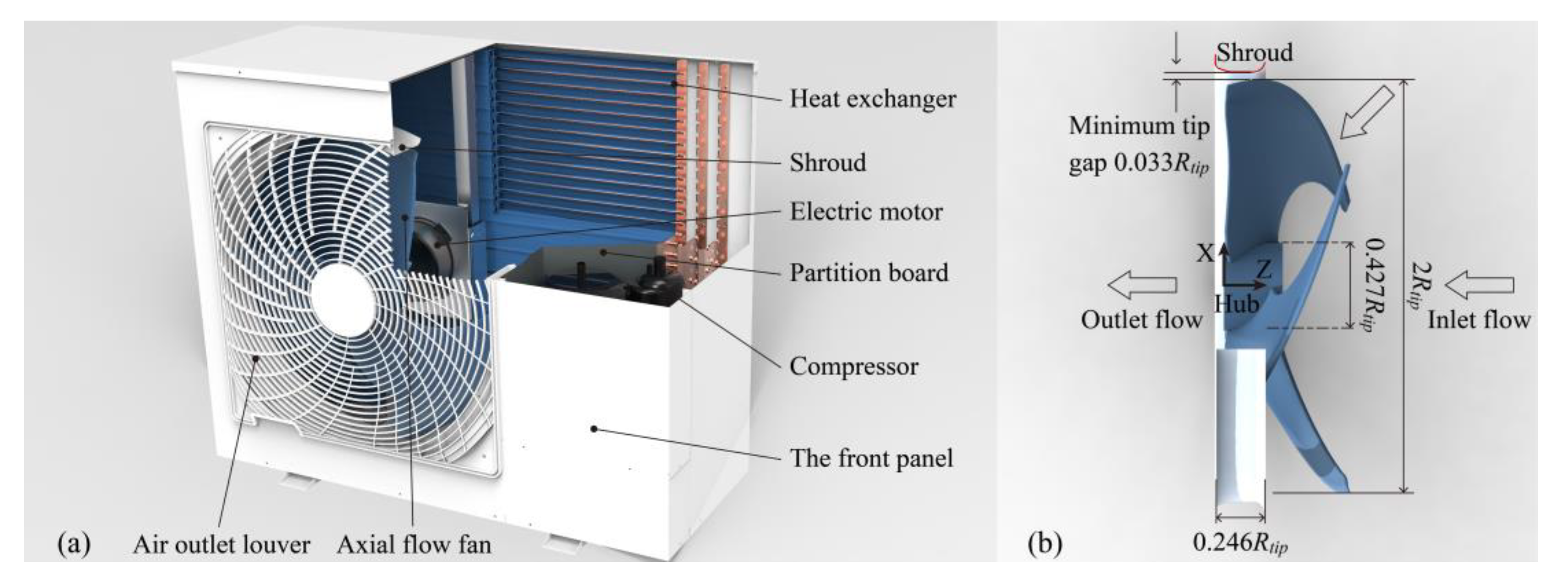
Figure 2.
Schematic diagram of the bionic forked trailing edge: (a) The forked fish caudal fin; (b) The blade with the bionic forked trailing edge.
Figure 2.
Schematic diagram of the bionic forked trailing edge: (a) The forked fish caudal fin; (b) The blade with the bionic forked trailing edge.

Figure 3.
Experimental setup for aerodynamic performance: (a) Schematic diagram of the fan aerodynamic test rig; (b) Photograph of the experimental facility.
Figure 3.
Experimental setup for aerodynamic performance: (a) Schematic diagram of the fan aerodynamic test rig; (b) Photograph of the experimental facility.
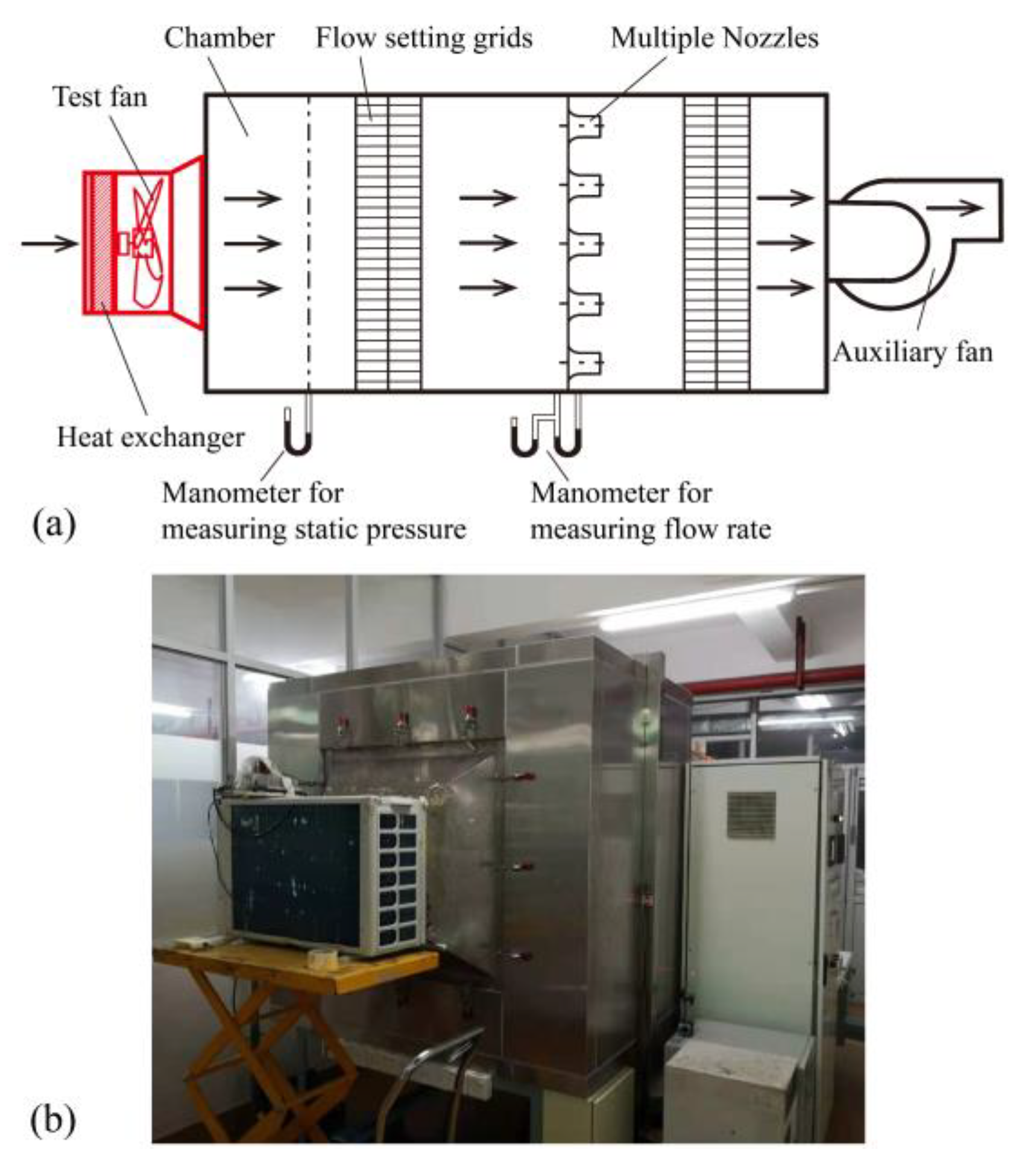
Figure 4.
Experimental setup for the aeroacoustic performance measurement in a semi-anechoic chamber.
Figure 4.
Experimental setup for the aeroacoustic performance measurement in a semi-anechoic chamber.

Figure 5.
Pressure drop with velocity in the finned-tube heat exchanger.

Figure 6.
Computational mesh of the axial flow fan: (a) Entire model of the computational zone, (b) Surface mesh of principal components, (c) Mesh on the blade surface.
Figure 6.
Computational mesh of the axial flow fan: (a) Entire model of the computational zone, (b) Surface mesh of principal components, (c) Mesh on the blade surface.

Figure 7.
Analysis of the mesh sensitivity: (a) Volume flow rate Qv, (b) y+ on the blade surface.

Figure 8.
Contour plot of y+ distributions on the blade surface under the rated operating condition Qv,r: (a) Pressure side, (b) Suction side.
Figure 8.
Contour plot of y+ distributions on the blade surface under the rated operating condition Qv,r: (a) Pressure side, (b) Suction side.

Figure 9.
Rotational speed n, shaft power W0, and power-saving rate γ distribution related to the angle of the bionic forked trailing edge θt at the rated operating condition Qv,r.
Figure 9.
Rotational speed n, shaft power W0, and power-saving rate γ distribution related to the angle of the bionic forked trailing edge θt at the rated operating condition Qv,r.

Figure 10.
Comparison between the predicted and experimental results: (a) Rotational speed n, (b) shaft power W0, and power-saving rate γ.
Figure 10.
Comparison between the predicted and experimental results: (a) Rotational speed n, (b) shaft power W0, and power-saving rate γ.

Figure 11.
Distribution of time-averaged static pressure on the pressure side (top) and suction side (bottom) between the prototype fan (left) and the BFT fan (right) at the rated operating condition Qv,r.
Figure 11.
Distribution of time-averaged static pressure on the pressure side (top) and suction side (bottom) between the prototype fan (left) and the BFT fan (right) at the rated operating condition Qv,r.

Figure 12.
Time-averaged static pressure distributions on different spans of the blade surface: (a) Span 48%, (b) Span 93%.
Figure 12.
Time-averaged static pressure distributions on different spans of the blade surface: (a) Span 48%, (b) Span 93%.

Figure 13.
The tip leakage flow rate distribution along the axial chord length.

Figure 14.
Distribution of time-averaged axial velocity at rotor outlet (z = 0 mm): (a) Prototype fan, (b) BFT fan. The black dotted line corresponds to the blade’s projection on this plane.
Figure 14.
Distribution of time-averaged axial velocity at rotor outlet (z = 0 mm): (a) Prototype fan, (b) BFT fan. The black dotted line corresponds to the blade’s projection on this plane.

Figure 15.
Time-averaged axial velocity distribution along spans at rotor outlet (z = 0 mm).

Figure 16.
The vortex structures of the rotor flow field identified by the iso-surfaces of Q = 3 × 10⁵ colored with velocity: (a) Prototype fan, (b) BFT fan.
Figure 16.
The vortex structures of the rotor flow field identified by the iso-surfaces of Q = 3 × 10⁵ colored with velocity: (a) Prototype fan, (b) BFT fan.

Figure 17.
Vorticity distribution on 96.4% span height (inside the tip clearance) of the rotor tip: (a) Prototype fan, (b) BFT fan. The horizontal white dashed line indicates the position of the shroud inlet.
Figure 17.
Vorticity distribution on 96.4% span height (inside the tip clearance) of the rotor tip: (a) Prototype fan, (b) BFT fan. The horizontal white dashed line indicates the position of the shroud inlet.

Figure 18.
Sound pressure levels (SPL), sound pressure level reduction value (△SPL) distribution related to the volume flow rate Qv.
Figure 18.
Sound pressure levels (SPL), sound pressure level reduction value (△SPL) distribution related to the volume flow rate Qv.

Figure 19.
Spectrum of prototype fan and BFT fan: (a) Sound pressure level spectrum and (b) 1/3 octave band sound pressure spectrum.
Figure 19.
Spectrum of prototype fan and BFT fan: (a) Sound pressure level spectrum and (b) 1/3 octave band sound pressure spectrum.


Table 1.
Main parameters of the axial flow fan.
| Parameter | Value |
|---|---|
| Number of blades | 3 |
| Blade tip radius, Rtip | 211mm |
| Rated operating condition, Qv,r | 2336 m3/h |
| Axial tip chord length, Cx/Rtip | 0.590 |
| Tip chord length, Ct/Rtip | 1.521 |
| Hub chord length, Ch/Rtip | 0.394 |
| Minimum tip celerance, tgap/Rtip | 0.033 |
| Hub-to-tip ratio, Rhub/Rtip Reynolds number, Re | 0.213 6.7 × 10⁴ |
Disclaimer/Publisher’s Note: The statements, opinions and data contained in all publications are solely those of the individual author(s) and contributor(s) and not of MDPI and/or the editor(s). MDPI and/or the editor(s) disclaim responsibility for any injury to people or property resulting from any ideas, methods, instructions or products referred to in the content. |
© 2023 by the authors. Licensee MDPI, Basel, Switzerland. This article is an open access article distributed under the terms and conditions of the Creative Commons Attribution (CC BY) license (https://creativecommons.org/licenses/by/4.0/).
Share and Cite
MDPI and ACS Style
Liang, Z.; Wang, J.; Wang, W.; Jiang, B.; Ding, Y.; Qin, W. Numerical and Experimental Investigations of Axial Flow Fan with Bionic Forked Trailing Edge. Machines 2023, 11, 155. https://doi.org/10.3390/machines11020155
AMA Style
Liang Z, Wang J, Wang W, Jiang B, Ding Y, Qin W. Numerical and Experimental Investigations of Axial Flow Fan with Bionic Forked Trailing Edge. Machines. 2023; 11(2):155. https://doi.org/10.3390/machines11020155
Chicago/Turabian StyleLiang, Zhong, Jun Wang, Wei Wang, Boyan Jiang, Yanyan Ding, and Wanxiang Qin. 2023. "Numerical and Experimental Investigations of Axial Flow Fan with Bionic Forked Trailing Edge" Machines 11, no. 2: 155. https://doi.org/10.3390/machines11020155
Note that from the first issue of 2016, this journal uses article numbers instead of page numbers. See further details here.