An Efficient Calculation Method for Stress and Strain of Concrete Pump Truck Boom Considering Wind Load Variation

Abstract

Digital twin is the development trend of concrete pump trucks to realize digitalization and intellectualization. The realization of digital twin requires high calculation efficiency and accuracy of the model. As the concrete pump truck works under the wind load, the wind speed and direction on site change frequently and intensely. However, existing methods, such as the finite element method, have the problems of low computational efficiency, high time complexity, and the update frequency being far lower than the frequency of wind change on site. We propose an efficient calculation model for the stress and strain of the pump truck boom based on the back propagation (BP) neural network. The novelty of this work is that when calculating the stress and strain of the boom, the change of the boom posture and the change of the site wind conditions are considered, and the calculation efficiency can be significantly improved. Compared with the finite element simulation, the fitting and prediction accuracy of the stress and strain are more than 99.7%, which can meet the requirements for real-time calculation of the stress and strain of the boom under different attitudes and wind loads in digital twins.

1. Introduction

1.1. Background

The concrete pump truck is a particular vehicle that uses pressure to transport and pour finished concrete along the boom pipe. It has the advantages of mobility, flexibility, high efficiency, and even continuous pouring. However, the working environment of the concrete pump truck is terrible, and boom retraction, boom extension, and posture switching cause boom fatigue. If the external wind load changes greatly, the boom may break, causing economic losses and, even, safety accidents [1]. However, the calculation accuracy and efficiency of the existing stress and strain calculation methods are challenging to take into account. Therefore, we propose an efficient calculation model for the stress and strain of boom to meet the requirements of digital twinning.

1.2. Formulation of the Problem of Interest for this Investigation

The commonly used method of stress and strain calculation is finite element simulation. However, the finite element method could be faster in calculation. In addition, it has high requirements for system hardware, which makes it difficult to provide real-time data for digital twins. Therefore, many scholars have improved the time integration algorithm to improve the accuracy and efficiency of the finite element calculation, simultaneously. For example, Li Zhibin et al. [2] improved the generalized d-method based on predictor-corrector and applied it to the finite element analysis of nonlinear structural dynamics, improving the stability and accuracy of calculation; Noh et al. [3] improved the accuracy of the implicit direct time integration method by adjusting the ratio of the time step. However, improving these algorithms still requires more work to meet the requirements of the calculation efficiency of the complex structure, and electromechanical and hydraulic coupling systems such as the concrete pump truck. Therefore, determining how to improve calculation efficiency under the premise of ensuring accuracy is an essential issue in realizing digital twinning.

1.3. Literature Survey

In recent years, AI (Artificial Intelligence) technologies based on data for analysis and prediction, have developed rapidly, showing significant advantages such as strong information extraction ability and fast processing speed [4]. In this context, the optimization technology based on proxy model has received more and more attention [5]. The basic idea of the proxy model is to collect many characteristic sample points from the data samples to construct a model that requires less computation and can replace the high-precision numerical model [6]. For example, Ying Wu et al. [7] used machine learning algorithms to analyze structural reliability problems in civil and mechanical engineering. Feng et al. [8] predicted the bridging stress by combining ANSYS and generalized regression neural network. Feng, S.Z., et al. [9] proposed a new method to predict the residual service life of structures by combining phase field method and depth learning.

1.4. Scope and Contribution of this Study

When the finite element method is used to calculate the stress and strain of the structure, the loading mode has a great influence on the calculation accuracy of the finite element method. For example, Zhang Yanwei et al. [10] carried out finite element modeling for each boom that was focused on the loading method of the boom structure model and gave the calculation method of the theoretical value of the stress of each boom under the most dangerous working conditions. However, when loading, the gravity of each boom and the end hose was regarded as the concentrated force acting on the midpoint, and the uneven wind load of the boom under different attitudes was not considered, which would increase the calculation error. Although Wei Liangbao et al. [11] regard weight as a uniformly distributed load, they ignore the problem of uneven mass distribution on the boom and do not consider the impact of wind load changes on the stress, strain, and stability of the boom system. Morooka et al. [12] proposed a new method for simulating the deformation of organ models by using a neural network. The neural network finds a relationship between external forces and the models deformed by the forces. The experimental results show that the trained network can achieve real-time simulation with a relative error of 9% compared with the nonlinear finite element calculation.

This paper takes a certain type of concrete pump truck boom system as the research object, focusing on the relationship between the stress and strain on the first boom and the boom attitude and wind load. The uneven distribution of mass on the boom is considered, and the boom is regarded as the uneven distribution of load. The influence of the change of wind direction and wind speed on the stress and strain of the boom is also considered.

1.5. Organization of the Paper

In Section 1, the mathematical model of the boom system is established first, and the relationship between the internal forces of each hinge point and each boom and the boom attitude is calculated according to the center of gravity position of each boom. In Section 2, 204 groups of typical attitudes and wind loads are selected, and the finite element method is used to calculate the stress and strain of each point on the boom 1# so as to determine the dangerous sections and dangerous points. Combining the mathematical model, the finite element simulation data is fitted to establish a proxy model to reduce the computational complexity and improve the computational efficiency [13]. Proxy models are used to mine the relationship between a large number of experimental data. In this paper, the proxy model based on LightGBM (light gradient boosting machine) machine learning, the proxy model based on the BP neural network, and the proxy model based on RBF (Radial Basis Function) neural network are, respectively, established. The modeling process and structural parameters of the three proxy models are described in detail in Section 3. In Section 4, the fitting and prediction accuracy of the three models under different structural parameters will be compared, and the differences in accuracy will be explained. In Section 5, some conclusions are drawn that the BP neural network proxy model can calculate the stress and strain of the key points of the boom structure more efficiently on the premise of ensuring accuracy.

2. Establishment of Mathematical Model of Boom System

2.1. Description of Concrete Pump Truck

The pump truck mainly comprises a chassis, pumping system, boom system, control system, hydraulic system, slewing mechanism, and outrigger [14]. The boom system is a conveying pipe that can rotate, fold, and expand. It can transport and pour concrete within a specific range. The boom system comprises connecting rods, hydraulic cylinders, boom plates, concrete conveying cylinders, and rubber hoses. Connecting rods, cylinder hinges, pin shafts, etc., can combine each boom. The structure of the pump truck boom system is complex. With the change in pumping conditions, the attitude of the boom is constantly changing, and its force is also changing. In addition, the pump truck boom system has two working modes. In the walking mode, the boom will be folded and placed on the chassis, with the outriggers close to both sides of the pump truck. In the pumping mode, the outriggers expand and support the equipment, and the boom extends to the designated position. The boom system will produce alternating stress when switching the working mode.

2.2. Degree of Freedom Analysis and Establishment of Coordinate System

The concrete pump truck boom system can be simplified into a turntable and six booms. The turntable has one degree of freedom, which can rotate on the horizontal plane. Each boom $i$ has one degree of freedom, which can rotate around the $i-1$ boom (boom 1# can rotate around the turntable through a rotary pair). The entire boom system has seven degrees of freedom. Let each rotation angle be in turn: a, ${\theta }_i$, where a is the rotation angle of the turntable on the horizontal plane (set as 0° forward in the initial state, increasing clockwise rotation), They are, respectively, the rotation angle of the boom $i$ relative to the boom $i-1$ (folded to 0° in the initial state, and increased in rotation and expansion, as shown in Figure 1, $\angle ABC={\theta }_1$, $\angle BCD={\theta }_2$, $\angle CDE={\theta }_3$, $\angle DEF={\theta }_4$, $\angle EFG={\theta }_5$, $\angle FGH={\theta }_6$, where the included angle between the boom 3# and the boom 4# is opposite to other included angles), and the boom 1#~6# are on the same plane, so the included angle j between each boom and the horizontal plane ($\angle ABC={\phi }_1$, $\angle ICD={\phi }_2$, $\angle JDE={\phi }_3$, $\angle KEF={\phi }_4$, $\angle LFG={\phi }_5$, $\angle MGH={\phi }_6$) can be calculated as follows:

$$\begin{gathered} {\phi }_1={\theta }_1 \\ {\phi }_2={\theta }_1+{\theta }_2–180° \\ {\phi }_3={\theta }_1+{\theta }_2+{\theta }_3–360° \\ {\phi }_4={\theta }_1+{\theta }_2+{\theta }_3–{\theta }_4–180° \\ {\phi }_5={\theta }_1+{\theta }_2+{\theta }_3–{\theta }_4+{\theta }_5–360° \\ {\phi }_6={\theta }_1+{\theta }_2+{\theta }_3–{\theta }_4+{\theta }_5+{\theta }_6–540° \end{gathered}$$

(1)

The boom section is considered as a box structure. Let the length of the boom $i$ be $l_i$, and the mass of the boom $i$ be $m_i$$(1\le i\le 6)$, and the width and height of the boom be $w_i$ and $h_i$, and define its center of gravity position coefficient as $P_i$($0\le P_i\le 1$), which represents the ratio of the position of the center of gravity to the hinge point of the previous boom and the total length of the boom (as shown in Figure 2).

2.3. Internal Force Analysis

2.3.1. Internal Force of Hinge Point

Dynamic programming method and static balance method are used to calculate the internal force of each boom. For the boom 6#, the H end is subjected to the downward tension of the end hose and the concrete $F_H$, its own gravity $m_{6}g$, and the vertical upward concentrated force $F_G$ and torque $T_G$ provided by the G end.

According to the conditions of static balance: (as shown in Figure 3)

$$F_G=m_{6}g+F_H$$

(2)

$$T_G=F_H{l}_6\cos {\phi }_6+m_{6}g{l}_6{P}_6\cos {\phi }_6$$

(3)

The values of $F_G$ and $T_G$ can be calculated.

Similarly, taking boom 5# as the research object, we can calculate:

$$F_F=m_{5}g+F_G$$

(4)

$$T_F=F_G{l}_5\cos {\phi }_5+m_{5}g{l}_5{P}_5\cos {\phi }_5+T_G$$

(5)

Bring in the $F_G$ and $T_G$ above to get:

$$F_F=m_{5}g+m_{6}g+F_H$$

(6)

$$T_F=(m_{6}g+F_H)l_5\cos {\phi }_5+m_{5}g{l}_5{P}_5\cos {\phi }_5+F_H{l}_6\cos {\phi }_6+m_{6}g{l}_6{P}_6\cos {\phi }_6$$

(7)

By analogy, the internal forces and moments of each hinge point can be obtained.

2.3.2. Boom Internal Force

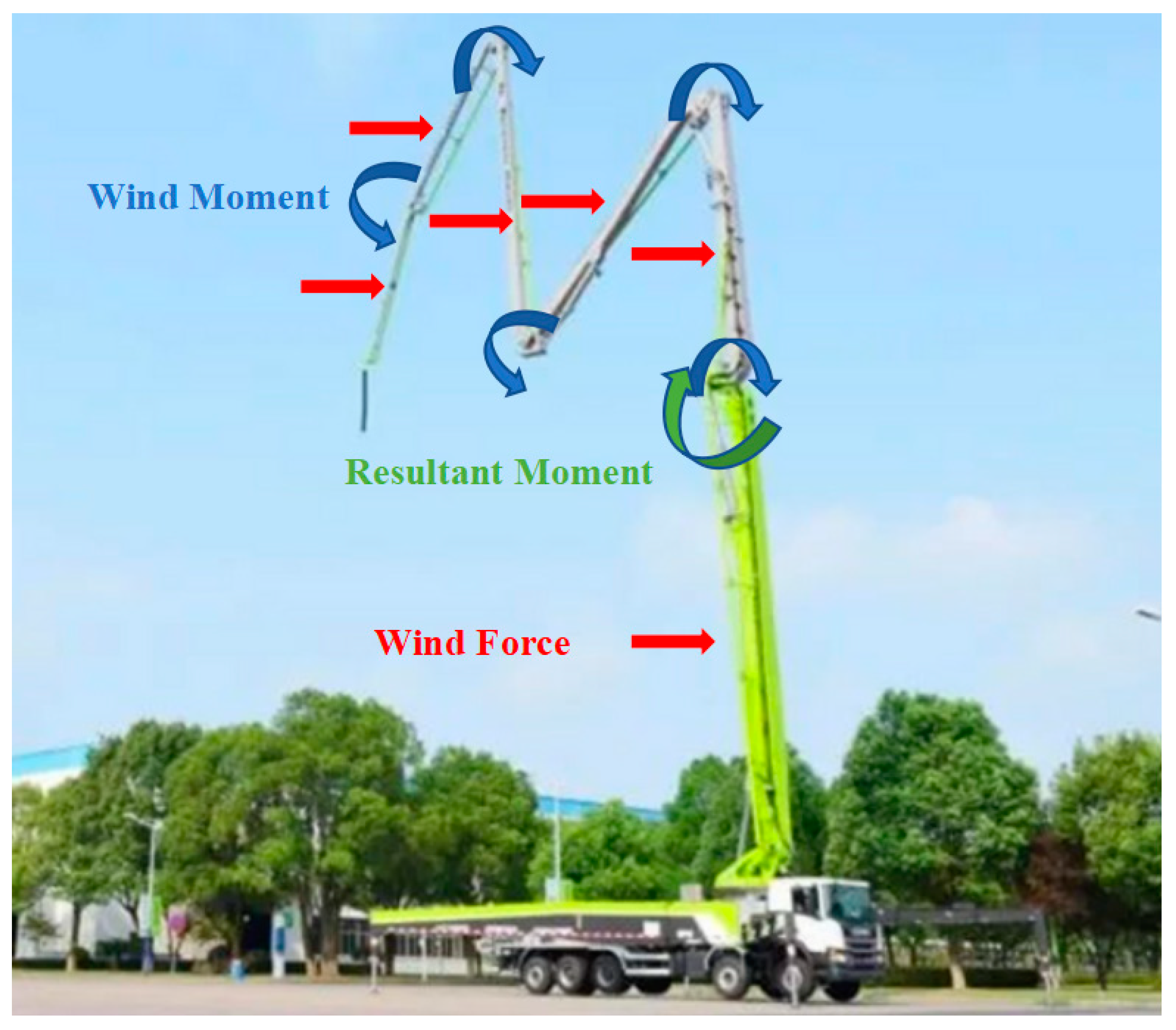
Booms 1#~6# are in the same plane, and axial force, shear force, and bending moment shall be considered for each boom.

For boom 6#, the maximum axial pressure on the boom is:

$$F_A=(m_{6}g+F_H)\sin {\phi }_6$$

(8)

The maximum shear force is:

$$F_S=(m_{6}g+F_H)\cos {\phi }_6$$

(9)

The maximum bending moment is:

$$M_G=F_H{l}_6\cos {\phi }_6+m_{6}g{l}_6{P}_6\cos {\phi }_6$$

(10)

The points with maximum force are located at the hinge of boom 5# and boom 6#.

In the same way, we can calculate the internal force of each other boom. The force of each force bearing point is given by the function $F=(i,u,{\theta }_k),i\le k\le 6$, where the parameter i represents the boom i#, u represents the division along the boom length, represents the ratio of the distance from the position to the hinge point of the upper boom to the boom length (for example, u = 0.5 represents the midpoint,$0\le u\le 1$), and the parameter ${\theta }_k$ represents the relative angle between the boom k# and the boom k − 1# (as shown in Figure 4).

2.3.3. Wind Load

During the actual working process of the pump truck, the boom system will be loaded due to the changes in the wind speed and direction of the external environment. The wind load has a great influence on the stress of the boom system and the stability during pumping, so it is necessary to consider and calculate the force of the wind load on the boom system and the moment it produces.

According to the national standard Load Code for the Design of Building Structures (GB 50009-2012), the standard value of wind load on main load-bearing structures:

$$w_k={\beta }_z{\mu }_s{\mu }_z{w}_0$$

(11)

where $w_k$ is standard value of wind load ($\mathrm{kN}/{{m}}^2$), ${\beta }_z$ is wind vibration coefficient at height z, ${\mu }_s$ is Wind load shape coefficient, ${\mu }_z$ is Variation coefficient of wind pressure height, $w_0$ is Basic wind pressure ($\mathrm{kN}/{{m}}^2$).

Wherein, the basic wind pressure

$$w_0=\frac{1}{2}\rho v_0^2$$

(12)

where $\rho$ is the air density, which can be estimated approximately from

$$\rho =0.00125e^{-0.0001z}$$

(13)

and z is the local altitude; $v_0$ is the basic wind speed, and its recurrence period should be 50 years. When the anemometer is used to observe the wind speed, its standard height should be 10 m. When the observed anemometer height differs greatly from the standard height, conversion is required:

$$v=v_z{(\frac{10}{z})}^{\alpha }$$

(14)

where: $z$ is actual height of anemometer (m), $v_z$ is Wind speed observed by anemometer (m/s), $\alpha$ is Surface roughness index of open and flat area, taking 0.15.

In addition, the wind direction has a great impact on the stability of the boom system, and the lateral wind, due to the largest windward area and the longest arm, and is very likely to cause large amplitude vibration of the boom. The longitudinal wind has little influence on the boom system due to its short force arm and small windward area, which can be ignored. The vertical component of wind is small and can also be ignored.

Assume that the force of wind load on the boom i# is $F_{wi}=w_k{S}_i\sin \vartheta$, where $S_i$ is the area of the side surface of the boom i#, and $\vartheta$ is the angle between the direction of the turntable and the wind direction. Similarly, the internal force and moment of hinge point of boom 6# under wind load can be calculated:

$$\overrightarrow{F_{wG}}=\overrightarrow{F_{w6}}+\overrightarrow{F_{wH}}$$

(15)

$$\overrightarrow{T_{wG}}=\overrightarrow{F_{w6}}{l}_6{P}_{w6}+\overrightarrow{F_{wH}}{l}_6$$

(16)

where $P_{wi}$ is the wind action location coefficient of boom i# (for example, $P_{wi}=\frac{1}{2}$ representing the midpoint, $0\le P_{wi}\le 1$). The shear force generated by wind load is:

$$F_{wS}=\left|\overrightarrow{F_{wG}}\right|$$

(17)

and the bending moment generated is:

$$M_{wG}=\overrightarrow{F_{wH}}{P}_{wH}{l}_H+\overrightarrow{F_{w6}}{P}_{w6}{l}_6$$

(18)

By analogy, the resultant moment on arm 1 can be obtained, as shown in Figure 5.

2.4. Stress and Deflection Analysis

Basic assumptions:

(1)

Continuity, the materials constituting the boom structure fill the volume of the boom without any gap.

(2)

Uniformity: the material mechanical properties of any part of each arm are the same.

(3)

Isotropic: The mechanical properties of materials are the same in all directions.

(4)

Linear elasticity, small deformation: the material is subject to linear elastic deformation, and the deformation amplitude is far less than the size of the boom.

The boom stress is divided into normal stress and shear stress. The size of the normal stress mainly depends on the axial force and bending moment. The axial normal stress is considered to be evenly distributed along the cross section of the boom, and the specified tensile stress is positive; The bending stress is considered as a linear distribution in the bending plane.

Take the boom 6# as an example, the maximum normal stress it receives:

$$\frac{F_A}{w_6{h}_6}+\frac{M_G{y}_{\max }}{I_Z}$$

(19)

$$y_{\max }=\frac{1}{2}{h}_6$$

(20)

where $I_Z$ is the moment of inertia. For a rectangular section,

$$I_Z=\frac{w_6{h}_6^3}{12}$$

(21)

the maximum shear stress it receives is

$$\tau =\frac{F_S{S}_Z^{*}}{w{I}_Z}$$

(22)

Make a line parallel to the $z$ axis through the calculation point, and the static moment of the other side of the line containing the $z$ axis (as shown in the red part in Figure 6) relative to the $z$ axis is $S_Z^{*}$.

With this method, the stress at each position of each boom can be calculated. The stress at each point is given by a function $F=(i,u,h,b,{\theta }_k),i\le k\le 6$, where the parameter h represents the fraction along the height of the cross section of the boom, and represents the ratio of the distance from the position to the bottom of the boom to the height of the cross section at that position, The parameter b represents the division along the width of the cross section of the boom (it is specified that $b$ = 0 represents the end face corresponding to the counterclockwise rotation of the symmetrical plane along the turntable, $b$ = 0.5 represents the symmetrical plane, and $b$ = 1 represents the end face corresponding to the clockwise rotation of the symmetrical plane along the turntable). Obviously, the normal stress reaches the maximum at the edge of the boom section ($h$ = 1 or 0), while the shear stress reaches the maximum at the center of the boom ($h$ = 0.5).

Take boom 1# as an example, the maximum deflection must occur at the hinge point of boom 1# and boom 2#, namely point C. Under small deformation, the bending angle is obtained from the integral of bending moment:

$$\theta =\tan \theta ={\displaystyle \int \frac{Mdx}{EI}}$$

(23)

The deflection and bending moment satisfy the differential equation:

$$\frac{d^{2}y}{d{x}^2}=\frac{M}{EI}$$

(24)

3. Simulation Analysis Based on ANSYS

The simulation analysis is carried out with boom 1# as the research object. The moment of booms 2~6# acting on boom 1# is

$$M_i={\displaystyle \sum _{k=2}^i{m}_{i}g{l}_k{P}_k\cos {\phi }_k}$$

(25)

the maximum moment $T_{\max }$ when booms 2~6# are parallel to the ground, and the minimum moment $T_{\min }$ when booms 2~6# are perpendicular to the ground. The moment is divided into 12 groups $T_0~T_{11}$(

Table 1. Moment Grouping.

Moment	${\mathit{T}}_0$	${\mathit{T}}_1$	${\mathit{T}}_2$	${\mathit{T}}_3$	${\mathit{T}}_4$	${\mathit{T}}_5$	${\mathit{T}}_6$	${\mathit{T}}_7$	${\mathit{T}}_8$	${\mathit{T}}_9$	${\mathit{T}}_{10}$	${\mathit{T}}_{11}$
Nm	0	60,000	120,000	180,000	240,000	300,000	360,000	420,000	480,000	540,000	600,000	660,000

). The force F acting on boom 1# is always the sum of gravity of booms 2~6#. In addition, it is necessary to consider the force and lateral moment of crosswind on booms 2~6#. The wind force is divided into 5 groups, and the minimum is $F_{w0}$, the maximum is $F_{w4}$(

Table 2. Wind Force Grouping.

Wind Force	${\mathit{F}}_{\mathit{w}0}$	${\mathit{F}}_{\mathit{w}1}$	${\mathit{F}}_{\mathit{w}2}$	${\mathit{F}}_{\mathit{w}3}$	${\mathit{F}}_{\mathit{w}4}$
N	0	1000	2000	3000	4000

). When the wind force exists, the average acting moment is divided into four groups according to the distance from the average acting position of the cross wind on the boom to point B, the minimum is $X_0$, and the maximum is $X_4$(

Table 3. Wind Average Force Arm Grouping.

Wind Average Acting Moment	${\mathit{X}}_0$	${\mathit{X}}_1$	${\mathit{X}}_2$	${\mathit{X}}_3$	${\mathit{X}}_4$
m	0	10	20	30	40

), so as to calculate the cross wind moment

$$T_w(i,j)=F_{wi}{X}_j$$

(26)

Load the above loads on the connection of booms 1# and 2#, that is, point C, and a total of 204 combinations are obtained. Hypermesh is used to mesh the boom 1# solid model. Add a fixed constraint at the connection between the boom 1# and the turntable (point B), and add the above load combination at point C. The wind load is divided into the concentrated force $F_{\mathrm{wc}}$ at point C and the uniformly distributed force $F_{\mathrm{wd}}$ on the boom 1# according to the side area of the boom (as shown in Figure 7). Use Hypermesh to convert the hm mesh file into a cdb file and import it into ANSYS. Use the Solution—Current LS function in ANSYS to solve the cdb file. The post processor of ANSYS is used to solve the maximum VonMisses equivalent stress of each node and calculate its maximum deformation. VonMisses equivalent stress is the equivalent stress obtained according to the fourth strength theory, which is applicable to plastic materials.

$$\sigma =\sqrt{\frac{1}{2}\left[{\left({\sigma }_1-{\sigma }_2\right)}^2+{\left({\sigma }_2-{\sigma }_3\right)}^2+{\left({\sigma }_1-{\sigma }_3\right)}^2\right]}$$

(27)

4. Construction and Optimization of a Surrogate Model

4.1. Data Preparation

In order to accelerate the convergence speed of the model, avoid neuron saturation, and facilitate the adjustment of the learning rate, it is necessary to normalize and standardize the original data, and map the data to the interval of [0,1] through Min Max Normalization:

$$X^{\prime }=\frac{X-X_{\min }}{X_{\max }-X_{\min }}$$

(28)

The Z-score method was used to standardize the data:

$$X^{\prime }=\frac{X-\mu }{\sigma }$$

(29)

Of the original data, 75%, namely 153 groups, were randomly selected as the training set, and the remaining 25%, namely 51 groups, were used as the verification set. In addition, 20 groups of parameter simulations within the scope $\{\begin{array}{l}0\le T\le 6.6\times {10}^5\mathrm{Nm}\\ 0\le F_w\le 4000 \mathrm{N}\\ 0\le X\le 40 \mathrm{m}\end{array}$ are randomly selected as the test set to test the generalization performance of the model, and 20 groups of parameter simulations within the scope $\{\begin{array}{l}6.6\times {10}^5 \mathrm{Nm}\le T\le {10}^6 \mathrm{Nm}\\ 4000\le F_w\le 5000 \mathrm{N}\\ 40\le X\le 50 \mathrm{m}\end{array}$ are randomly selected to test the prediction performance of the model to predict the stress and strain caused by the actual loading of the boom due to impact and dynamic load under the actual working conditions.

4.2. Machine Learning Proxy Model Based on LightGBM

Qi [15] first proposed LightGBM in 2017. LightGBM is a framework for implementing GBDT (gradient boosting decision tree) algorithm, and the main idea of GBDT is to use decision tree iterative training to obtain the optimal model. The traditional GBDT algorithm needs to traverse the entire data multiple times in each iteration. When the data volume is large, it is difficult to put the entire data into memory, and frequent calls to disk for reading and writing will reduce the efficiency. LightGBM uses the Histogram algorithm for optimization (Figure 8). Its basic idea is to discretize the continuous floating-point eigenvalues into k integers, and construct a histogram with a width of k. When traversing the data, the discretized value is used as the index to accumulate statistics in the histogram. After traversing the data once, the histogram accumulates the required statistics, and then traverses to find the optimal partition point according to the discrete value of the histogram. Histogram algorithm does not need additional storage of presorted results, which can significantly reduce memory consumption; Secondly, it can greatly reduce the calculation time. The presorting algorithm needs to calculate a split gain every time it traverses an eigenvalue, while the histogram algorithm only needs to calculate a constant number of times, and the time complexity is optimized from O (#data*#feature) to O (k*#features).

In addition, LightGBM abandoned the level-wise (Figure 9a) decision tree growth strategy used by most GBDT tools and replaced it with the leaf-wise (Figure 9b) algorithm. The purpose of layer-by-layer growth is to facilitate the control of the complexity of the model, prevent the occurrence of overfitting, and facilitate the multi-threaded optimization. However, its efficiency still has room for improvement because it treats the same layer of leaves indiscriminately, and the benefits of searching and splitting some leaves in the same layer are low, which brings a lot of unnecessary expenses. The algorithm of growing by leaves is to find a leaf with the largest split income among all the current leaves. Under the same split times, the fitting accuracy of the strategy of growing by leaves is greater than that of the strategy of growing by layers. In order to prevent the growth of decision trees with excessive depth and overfitting, LightGBM adds the limitation of maximum tree depth [16].

The parameters in the experiment include the maximum number of leaves and the maximum tree depth. The other parameters are shown in the results section.

4.3. A Proxy Model Based on the BP Neural Network

The structure of the proxy model based on the BP neural network is shown in Figure 10. As shown, each layer contains several neurons. The first layer is the input layer which contains three inputs of moment $T$, wind load $F_w$, and wind moment $T_w$. The middle layer is the hidden layer, and the last layer is the output layer, where a represents the maximum equivalent stress and x represents the maximum deformation [17,18]. The hidden layer is generally one or two layers. The one hidden layer (Figure 10a) can approximate any function that contains a continuous mapping from one finite space to another, while the two hidden layer (Figure 10b) can represent an arbitrary decision boundary to arbitrary accuracy with rational activation functions and can approximate any smooth mapping to any accuracy. Increasing the number of network layers will enhance the fitting ability of the network, but will increase the training difficulty, and more likely bring about the problem of overfitting.

In order to introduce nonlinear elements into the network, activation functions (Figure 11) are needed. The commonly used activation functions are given as:

(1)

Softplus activation function:

$$f(x)=\ln (1+e^x).$$

(30)

(2)

Relu activation function:

$$f(x)=\{\begin{array}{l}x,x\ge 0\\ 0,x<0\end{array}$$

(31)

(3)

Sigmoid activation function:

$$f(x)=\frac{1}{1+e^{-x}}$$

(32)

(4)

Tanh activation function:

$$f(x)=\frac{1-e^{2x}}{1+e^{2x}}$$

(33)

Figure 11. Activation functions.

Figure 11. Activation functions.

In this paper, MSE (mean squared error) is used as the loss function, Adam (adaptive moment estimation) and SGD (stochastic gradient descent) optimizers are used, respectively. By changing the combination of the number of neurons and the number of hidden layers in the network, the influence of different training times on the model fitting accuracy and prediction accuracy is studied, and the optimal parameters are sought.

The formula of the Adam optimizer can be expressed as:

$$g_t=\nabla \widehat{L}({\theta }_t).$$

(34)

$$m_t={\beta }_1{m}_{t-1}+(1-{\beta }_1)g_t$$

(35)

$$v_t={\beta }_2{v}_{t-1}+(1-{\beta }_2)g_t^2$$

(36)

$$\widehat{m_t}=\frac{m_t}{1-{\beta }_1^t}$$

(37)

$$\widehat{v_t}=\frac{v_t}{1-{\beta }_2^t}$$

(38)

$${\theta }_{t+1}={\theta }_t-\frac{\eta }{\sqrt{\widehat{v_t}}+\epsilon }\widehat{m_t}$$

(39)

$$MSE=\frac{1}{2n}{\displaystyle \sum _{i=1}^n{f}^2({\sigma }_i)}$$

(40)

The Adam optimizer parameter setting: initial learning rate 0.002, ${\beta }_1$ = 0.9, ${\beta }_2$ = 0.999.

The SGD optimizer parameters are: Learning rate = 0.002, Momentum = 0.9.

Other parameters are shown in the results section.

4.4. A Proxy Model Based on the RBF Neural Network

The RBF neural network is a three-layer neural network, which includes the input layer, the hidden layer and the output layer [19], as shown in the Figure 12. The transformation from input space to hidden space is nonlinear, while the transformation from hidden space to output space is linear. The difference between an RBF neural network and a traditional BP neural network is that the former uses the radial basis function as the activation function during forward propagation. Radial basis function is a scalar function that is symmetrical along the radial direction. It is usually a Euclidean distance monotone function from a point in space to a center, which can be recorded as $K\left|\left|X-X_c\right|\right|$. The most commonly used radial basis function is a Gaussian kernel function (Figure 13).

$$K\left|\left|X-X_c\right|\right|=e^{-\frac{{\left|\left|X-X_c\right|\right|}^2}{2{\sigma }^2}}$$

(41)

As shown, s reflects the width of the function image. The smaller s is, the narrower the width is, and the more selective the function is.

The RBF network in this paper uses Adam and SGD optimizer to achieve the best accuracy by changing the training times and learning rate parameters. The momentum coefficient of SGD is 0.9, and the formula is:

$$v_{dW}=\beta v_{dW}+(1-\beta )dW$$

(42)

$$v_{db}=\beta v_{db}+(1-\beta )db$$

(43)

$$W=W-a{v}_{dW}$$

(44)

$$b=b-\alpha v_{db}$$

(45)

5. Results and Discussion

5.1. Simulation Results of Stress and Strain

Figure 14 shows that both wind force and wind action moment will significantly increase the stress and strain of the key points of the boom, and when the wind action moment increases, the nonlinear relationship between the boom strain and the hinge point moment gradually increases.

Table 4. The influence of center of gravity position coefficient on stress and strain in horizontal attitude.

${\mathit{P}}_{\mathit{i}}(\mathit{i}=1,2,\mathrm{\dots },6)$	0.4	0.45	0.5	0.55	0.6
Stress (Mpa)	597.060	607.291	617.522	627.753	637.985
Strain (mm)	147.961	150.683	153.405	156.128	158.850

shows that the center of gravity position coefficient has a certain influence on the stress and strain of the boom under the horizontal attitude. When the center of gravity position coefficient increases, the force arm of gravity increases, which leads to the increase of stress and strain. Therefore, the non-uniformity of the mass distribution of the boom should not be ignored.

5.2. Results of LightGBM

The experimental data of LightGBM are shown in

Table 5. The quality assessment of LightGBM models with various configurations.

Configuration	Learning Rate	Training Times	Lambda_l2	Stress Fitting Error%	Strain Fitting Error%	Stress Prediction Error%	Strain Prediction Error%	Training Time
1	0.05	1000	0.6	−0.206	−1.133	−19.063	−18.077	0.7 s
2	0.05	2000	0.6	−0.260	−1.118	−18.419	−17.434	1.1 s
3	0.05	3000	0.6	−0.267	−1.107	−18.175	−17.299	1.5 s
4	0.05	4000	0.6	−0.267	−1.107	−18.083	−17.233	1.7 s
5	0.05	5000	0.6	−0.257	−1.112	−18.022	−17.201	3.3 s
6	0.01	5000	0.6	3.347	−1.259	−17.682	−17.226	2.2 s
7	0.01	10,000	0.6	−0.233	−1.091	−18.300	−17.464	3.4 s
8	0.01	15,000	0.6	−0.224	−1.094	−18.226	−17.332	5.2 s
9	0.01	20,000	0.6	−0.231	−1.118	−18.105	−17.223	6.4 s
10	0.01	25,000	0.6	−0.211	−1.119	−18.055	−17.210	8.3 s
11	0.05	5000	0.2	−0.186	−1.121	−18.024	−17.211	2.6 s
12	0.05	5000	0.4	−0.265	−1.092	−18.035	−17.212	2.2 s
13	0.05	5000	0.8	−0.186	−1.075	−18.040	−17.199	2.5 s
14	0.05	5000	1	−0.268	−1.099	−18.040	−17.192	2.5 s

. On the whole, the LightGBM model has fast training speed, small fitting error, but large prediction error. Increasing the training times will slightly reduce the fitting error and prediction error. If you increase the training times and reduce the learning rate, the effect of error reduction will be more obvious. In addition, changing the value of Lambda_l2 has no obvious impact on the accuracy of the model because the depth of the tree oscillates between 4 and 5 during training, and the number of leaves oscillates between 5 and 6, both of which do not reach the set maximum value and do not produce overfitting.

Note that all the prediction results of LightGBM for the prediction set are the same. The reason is that the values of the prediction dataset are larger than the training set, and the leaf nodes are limited. During training, continuous data sets are mapped to leaf nodes by dichotomy. When the prediction data exceeds the range of the training data set, it will be mapped to the leaf node corresponding to the maximum value of the training data set, so the prediction output is always a certain value. This will make the model lack of prediction ability.

5.3. Results of BP

The experimental data of BP neural network are shown in

Table 6. The quality assessment of BP Neural Network models with various configurations.

Configuration	Training Times	Optimizer	Activation Function	Layer(s)	Hidden Layer Size	Training Set MSE Loss	Validation Set MSE Loss	Stress Fitting Error%	Strain Fitting Error%	Stress Prediction Error%	Strain Prediction Error%	Training Time
1	5000	Adam	Softplus	1	4	1.96 × 10−3	2.28 × 10−3	0.084	−0.257	−0.954	−2.889	24.2 s
2	10,000	Adam	Softplus	1	4	6.02 × 10−4	7.73 × 10−4	0.040	−0.212	0.288	−0.699	43.8 s
3	15,000	Adam	Softplus	1	4	5.96 × 10−4	7.01 × 10−4	−0.100	−0.170	−0.203	0.015	65.9 s
4	20,000	Adam	Softplus	1	4	5.62 × 10−4	3.83 × 10−4	−0.253	−0.330	0.263	0.143	87.8 s
5	5000	SGD	Softplus	1	4	3.76 × 10−3	3.77 × 10−3	0.022	−0.293	−3.555	−4.355	16.2 s
6	10,000	SGD	Softplus	1	4	2.98 × 10−3	2.64 × 10−3	0.100	−0.166	−2.073	−2.288	32.9 s
7	15,000	SGD	Softplus	1	4	3.22 × 10−3	2.65 × 10−3	−0.124	−0.358	−3.389	−4.407	49.6 s
8	20,000	SGD	Softplus	1	4	2.50 × 10−3	2.33 × 10−3	0.010	−0.296	−2.843	−3.437	63.4 s
9	5000	Adam	Softplus	1	6	5.06 × 10−4	7.28 × 10−4	0.017	0.032	−1.462	−1.262	26.1 s
10	10,000	Adam	Softplus	1	6	1.41 × 10−4	2.27 × 10−4	−0.126	−0.041	−0.584	−1.113	51.9 s
11	15,000	Adam	Softplus	1	6	1.11 × 10−4	1.49 × 10−4	−0.017	−0.241	−0.408	−1.038	79.3 s
12	20,000	Adam	Softplus	1	6	8.72 × 10−5	1.09 × 10−4	−0.093	−0.207	−0.377	−0.080	111.1 s
13	5000	Adam	Softplus	1	8	8.09 × 10−5	9.56 × 10−5	−0.048	−0.217	−1.402	−1.769	26.4 s
14	10,000	Adam	Softplus	1	8	6.42 × 10−5	7.54 × 10−5	−0.030	−0.229	−0.653	−0.697	52.2 s
15	15,000	Adam	Softplus	1	8	7.35 × 10−5	8.86 × 10−5	−0.003	−0.263	−0.756	−1.116	79.7 s
16	20,000	Adam	Softplus	1	8	5.65 × 10−5	7.62 × 10−5	0.069	−0.223	−0.592	−1.075	106.8 s
17	5000	Adam	Softplus	1	10	6.95 × 10−5	8.16 × 10−5	0.003	−0.243	−0.436	−0.811	26.7 s
18	10,000	Adam	Softplus	1	10	5.40 × 10−5	7.20 × 10−5	−0.033	−0.291	−0.808	−0.691	53.1 s
19	15,000	Adam	Softplus	1	10	6.43 × 10−5	8.19 × 10−5	0.087	−0.272	−0.362	−1.629	80.2 s
20	20,000	Adam	Softplus	1	10	4.25 × 10−5	4.31 × 10−5	0.006	−0.336	−0.620	−1.277	107.3 s
21	5000	Adam	Softplus	1	12	8.30 × 10−5	1.04 × 10−4	-0.375	−0.269	−0.140	−1.398	26.4 s
22	10,000	Adam	Softplus	1	12	4.67 × 10−5	4.71 × 10−5	0.097	−0.308	−0.125	−0.872	55.7 s
23	15,000	Adam	Softplus	1	12	3.53 × 10−5	4.09 × 10−5	−0.012	−0.358	−0.416	−0.717	79.9 s
24	20,000	Adam	Softplus	1	12	4.51 × 10−5	4.29 × 10−5	0.078	−0.321	0.012	−0.532	109.8 s
25	10,000	Adam	Sigmoid	1	12	4.53 × 10−5	4.06 × 10−5	0.070	−0.110	−2.216	−1.180	52.7 s
26	10,000	Adam	Relu	1	12	1.61 × 10−4	3.68 × 10−4	0.203	0.135	−3.039	−2.645	52.6 s
27	10,000	Adam	Tanh	1	12	6.05 × 10−5	7.68 × 10−5	−0.051	−0.053	−5.237	−3.368	51.9 s
28	5000	Adam	Softplus	2	4 + 2	8.90 × 10−4	1.15 × 10−3	0.284	0.007	−1.292	−2.057	27.2 s
29	10,000	Adam	Softplus	2	4 + 2	6.37 × 10−4	8.01 × 10−4	0.030	−0.134	0.242	−0.655	53.8 s
30	15,000	Adam	Softplus	2	4 + 2	4.68 × 10−4	6.14 × 10−4	−0.156	−0.321	−0.895	−0.717	81.4 s
31	20,000	Adam	Softplus	2	4 + 2	5.59 × 10−4	6.88 × 10−4	−0.009	−0.165	0.139	−0.871	108.1 s
32	5000	Adam	Softplus	2	6 + 3	2.42 × 10−4	3.35 × 10−4	−0.227	−0.244	0.255	−0.006	32.6 s
33	10,000	Adam	Softplus	2	6 + 3	1.15 × 10−4	1.38 × 10−4	−0.122	−0.201	−0.194	−0.411	64.9 s
34	15,000	Adam	Softplus	2	6 + 3	9.65 × 10−5	1.17 × 10−4	0.022	−0.289	−0.783	−0.799	97.4 s
35	20,000	Adam	Softplus	2	6 + 3	1.43 × 10−4	1.67 × 10−4	0.009	−0.232	−0.555	−0.093	129.2 s
36	5000	Adam	Softplus	2	8 + 4	1.25 × 10−4	1.35 × 10−4	−0.085	−0.394	−0.896	−1.113	32.5 s
37	10,000	Adam	Softplus	2	8 + 4	8.67 × 10−5	9.72 × 10−5	0.009	−0.263	−0.361	−1.280	65.5 s
38	15,000	Adam	Softplus	2	8 + 4	6.48 × 10−5	8.62 × 10−5	−0.025	−0.425	−0.255	−1.226	99.5 s
39	20,000	Adam	Softplus	2	8 + 4	4.38 × 10−5	4.91 × 10−5	−0.207	−0.333	−0.022	−0.337	131.1 s
40	5000	Adam	Softplus	2	4 + 8	1.03 × 10−3	1.09 × 10−3	0.319	0.075	−0.420	−1.480	32.7 s
41	10,000	Adam	Softplus	2	4 + 8	6.27 × 10−4	6.99 × 10−4	−0.073	−0.221	0.141	−1.114	64.3 s
42	15,000	Adam	Softplus	2	4 + 8	6.28 × 10−4	7.87 × 10−4	0.055	−0.126	0.121	−0.820	96.6 s
43	20,000	Adam	Softplus	2	4 + 8	5.20 × 10−4	6.72 × 10−4	−0.144	−0.338	−0.601	−0.468	131.4 s

and Figure 15. On the whole, the training of BP network takes a long time, and the fitting accuracy and prediction accuracy are both high. The training time using SGD optimizer is shorter than Adam, but the prediction accuracy is lower than Adam. Because every time the SGD is updated, it will update each sample with gradient, so the SGD has a large noise and is greatly affected by a single sample, which may lead to repeated adjustment and oscillation of parameters, resulting in large randomness and low accuracy of the results, which may not necessarily tend to global optimization. The Adam optimizer, absorbing the advantages of Adagrad and momentum gradient descent algorithm, can not only adapt to the sparse gradient problem, but also alleviate the gradient oscillation problem, and can adaptively adjust the learning rate. The activation function using Softplus has the best prediction effect. Compared with the Relu activation function, it is more smooth. It solves the problem that neurons cannot update parameters when the input value is negative and retains the advantage that the Relu activation function converges faster. Compared with Sigmoid activation function, it solves the problem of saturation when the absolute value of input is too large. Increasing the number of hidden layer nodes and network layers will reduce the loss of the training set and the verification set, but it will also increase the prediction error of the model and increase the training time.

5.4. Results of RBF

The experimental data of RBF neural network is shown in

Table 7. The quality assessment of RBF Neural Network models with various configurations.

Configuration	Training Times	Optimizer	Learning Rate	Training Set MSE Loss	Validation Set MSE Loss	Stress Fitting Error%	Strain Fitting Error%	Stress Prediction Error%	Strain Prediction Error%	Training Time
1	2000	SGD	0.1	3.24 × 10−6	1.58 × 10−3	0.534	0.343	−1.262	0.294	5.8 s
2	4000	SGD	0.1	4.95 × 10−7	1.58 × 10−3	0.541	0.358	−1.245	0.281	6.7 s
3	6000	SGD	0.1	1.63 × 10−7	1.58 × 10−3	0.543	0.361	−1.247	0.271	9.5 s
4	8000	SGD	0.1	5.92 × 10−8	1.59 × 10−3	0.543	0.362	−1.250	0.265	12.8 s
5	1000	Adam	0.01	5.39 × 10−3	2.60 × 10−1	12.482	11.174	−22.159	−21.337	2.4 s
6	2000	Adam	0.01	3.76 × 10−3	3.03 × 10−1	11.832	11.095	−24.870	−23.845	4.4 s
7	3000	Adam	0.01	3.74 × 10−3	3.05 × 10−1	11.795	11.203	−25.555	−24.420	5.6 s
8	4000	Adam	0.01	3.64 × 10−3	3.41 × 10−1	12.079	12.109	−25.780	−24.775	7.2 s
9	2000	SGD	0.05	1.62 × 10−5	1.65 × 10−3	0.523	0.322	−1.272	0.340	3.7 s
10	4000	SGD	0.05	3.54 × 10−6	1.59 × 10−3	0.530	0.343	−1.243	0.314	6.6 s
11	6000	SGD	0.05	1.13 × 10−6	1.58 × 10−3	0.536	0.353	−1.227	0.309	10.5 s
12	8000	SGD	0.05	5.35 × 10−7	1.59 × 10−3	0.539	0.358	−1.223	0.303	12.6 s
13	10,000	SGD	0.05	3.00 × 10−7	1.59 × 10−3	0.540	0.361	−1.222	0.298	16.1 s
14	10,000	SGD	0.01	1.72 × 10−5	1.66 × 10−3	0.519	0.321	−1.258	0.353	15.9 s
15	20,000	SGD	0.01	3.81 × 10−6	1.59 × 10−3	0.527	0.342	−1.227	0.331	31.3 s
16	30,000	SGD	0.01	1.25 × 10−6	1.59 × 10−3	0.533	0.354	−1.209	0.327	48.8 s
17	40,000	SGD	0.01	6.42 × 10−7	1.59 × 10−3	0.535	0.358	−1.204	0.322	62.9 s

. In general, the training time of RBF network is shorter than that of BP network, and the fitting accuracy and prediction accuracy are slightly lower than that of BP neural network. SGD optimizer performs better than Adam on RBF network, and Adam optimizer is more prone to overfitting. In addition, increasing the number of trainings can reduce the prediction error, but the effect is limited which will reduce the fitting accuracy to a certain extent. The effect of changing the learning rate on the accuracy of the model is not obvious.

6. Conclusions

This paper proposes a proxy model for calculating the stress and strain of concrete pump truck boom system based on LightGBM, BP, and RBF, taking into account the varying wind load and mass boom distribution. Use simulation data to train the model. The model’s input consist of boom attitude, wind force, and wind torque, and the output is the stress and strain of critical points. The innovation of this method combines the mechanism model, simulation model, and artificial intelligence algorithm of the boom. It significantly improves stress and strain calculation efficiency at critical points to ensure calculation accuracy and meet real-time calculation requirements in digital twins. The following conclusions can be drawn:

• Among the above proxy models, the BP neural network with a single layer of four neurons has the highest accuracy. The fitting accuracy of stress is 99.900%, the fitting accuracy of strain is 99.830%, the prediction accuracy of stress is 99.797%, and the prediction accuracy of strain is 99.985%, which fully meets the calculation accuracy requirements in digital twins.
• The finite element simulation calculation takes at least 9 s, while the calculation time of the proxy model is less than 0.001 s. Compared with the finite element simulation method, the proxy model can significantly improve stress and strain calculation efficiency.
• From the perspective of the model training time, BP, RBF, and LightGBM are in order from long to short. In terms of fitting accuracy, BP, RBF, and LightGBM are in order from good to bad. From the perspective of prediction accuracy, BP, RBF, and LightGBM are in order from good to bad. The training time is positively correlated with the model accuracy, and the depth learning model has higher accuracy than the traditional machine learning model, but the training time is longer.
• The wind force and the wind force arm significantly impact the boom’s stress and strain, which can be more than twice as large.
• In the horizontal attitude, the uneven mass distribution of the boom will have a certain impact on its stress and strain. Every 0.1 times the length of the deviation from the geometric center, its stress and strain will change by more than 3%.

References

1. Hua, G. Research on Key Technology of Structure Health Monitoring for Boom of Concrete Pump Truck; Central South University: Changsha, China, 2013; p. 124. [Google Scholar]
2. Li, Z.; Jiang, P.; Pan, J.; Zhang, Q.; Zhao, G.; Guan, Z. The predictor-corrector scheme based Generalized-αmethod and its application in nonlinear structural dynamics. Chin. J. Comput. Mech. 2020, 37, 28–33. [Google Scholar] [CrossRef]
3. Noh, G.; Bathe, K.J. Further insights into an implicit time integration scheme for structural dynamics. Comput. Struct. 2018, 202, 15–24. [Google Scholar] [CrossRef]
4. Wang, K.; Guo, M.; Dai, C.; Li, Z. Information-decision searching algorithm: Theory and applications for solving engineering optimization problems. Inf. Sci. 2022, 607, 1465–1531. [Google Scholar] [CrossRef]
5. Kolajoobi, R.A.; Haddadpour, H.; Niri, M.E. Investigating the capability of data-driven proxy models as solution for reservoir geological uncertainty quantification. J. Pet. Sci. Eng. 2021, 205, 108860. [Google Scholar] [CrossRef]
6. Gupta, S.; Mukhopadhyay, T.; Kushvaha, V. Microstructural image based convolutional neural networks for efficient prediction of full-field stress maps in short fiber polymer composites. Def. Technol. 2022. [Google Scholar] [CrossRef]
7. Afshari, S.S.; Enayatollahi, F.; Xu, X.; Liang, X. Machine learning-based methods in structural reliability analysis: A review. Reliab. Eng. Syst. Saf. 2021, 219, 108223. [Google Scholar] [CrossRef]
8. Wu, Y.; Zhang, L.; Liu, H.; Lu, P. Stress prediction of bridges using ANSYS soft and general regression neural network. Structures 2022, 40, 812–823. [Google Scholar] [CrossRef]
9. Feng, S.; Xu, Y.; Han, X.; Li, Z.; Incecik, A. A phase field and deep-learning based approach for accurate prediction of structural residual useful life. Comput. Methods Appl. Mech. Eng. 2021, 383, 113885. [Google Scholar] [CrossRef]
10. Zhang, Y.; Tong, L.; Sun, G. A Structure Analysis of Concrete Pump’s Boom Based on ANSYS. J. Wuhan Univ. Technol. 2004, 28, 536–539. [Google Scholar]
11. Wei, L.; Gong, G.; Ren, P.; Si, Y.; Wan, X. Loading analysis on boom structure of concrete pump trucks. Chin. J. Constr. Mach. 2014, 12, 163–167. [Google Scholar] [CrossRef]
12. Morooka, K.; Chen, X.; Kurazume, R.; Uchida, S.; Hara, K.; Iwashita, Y.; Hashizume, M. Real-Time Nonlinear FEM with Neural Network for Simulating Soft Organ Model Deformation. In International Conference on Medical Image Computing and Computer-Assisted Intervention; Springer: Berlin/Heidelberg, Germany, 2008; Volume 11, pp. 742–749. [Google Scholar] [CrossRef] [Green Version]
13. Han, D.; Zheng, J. A Survey of Metamodeling Techniques in Engineering Optimization. J. East China Univ. Sci. Technol. 2012, 38, 762–768. [Google Scholar] [CrossRef]
14. Wu, Y.; Li, W.; Liu, Y. Fatigue life prediction for boom structure of concrete pump truck. Eng. Fail. Anal. 2016, 60, 176–187. [Google Scholar] [CrossRef]
15. Qi, M. LightGBM: A Highly Efficient Gradient Boosting Decision Tree. Neural Information Processing Systems; Curran Associates Inc.: Beijing, China, 2017. [Google Scholar]
16. Zhao, R.; Wei, D.; Ran, Y.; Zhou, G.; Jia, Y.; Zhu, S.; He, Y. Building Cooling load prediction based on LightGBM. IFAC-Pap. IFAC-Pap 2022, 55, 114–119. [Google Scholar] [CrossRef]
17. Xu, J.; Chen, Y.; Xie, T.; Zhao, X.; Xiong, B.; Chen, Z. Prediction of triaxial behavior of recycled aggregate concrete using multivariable regression and artificial neural network techniques. Constr. Build. Mater. 2019, 226, 534–554. [Google Scholar] [CrossRef]
18. Duan, Z.H.; Kou, S.C.; Poon, C.S. Prediction of compressive strength of recycled aggregate concrete using artificial neural network and cuckoo search method. Mater. Today Proc. 2021, 46, 8480–8488. [Google Scholar] [CrossRef]
19. Han, H.-G.; Ma, M.-L.; Qiao, J.-F. Accelerated gradient algorithm for RBF neural network. Neurocomputing 2021, 441, 237–247. [Google Scholar] [CrossRef]
Figure 1. The included angle between the booms and the angle relative to the horizontal plane.
Machines 11 00161 g001
Figure 2. Schematic diagram of center of gravity position coefficient.
Machines 11 00161 g002
Figure 3. (a) Stress Analysis of Boom 6#; (b) Stress Analysis of Boom 5#.
Machines 11 00161 g003
Figure 4. Schematic diagram of parameter i, u and θ k .
Machines 11 00161 g004
Figure 5. Resultant Moment on Boom 1#.
Machines 11 00161 g005
Figure 6. Schematic diagram of parameter S Z * interpretation.
Machines 11 00161 g006
Figure 7. Schematic diagram of boom restraint and load.
Machines 11 00161 g007
Figure 8. Histogram algorithm.
Machines 11 00161 g008
Figure 9. (a) Level-wise tree growth; (b) Leaf-wise tree growth.
Machines 11 00161 g009
Figure 10. (a) Single hidden layer BP neural network (b) Double hidden layer BP neural network.
Machines 11 00161 g010
Figure 12. RBF neural network.
Machines 11 00161 g012
Figure 13. Gaussian Radial Basis Function.
Machines 11 00161 g013
Figure 14. Relationship between stress (a) and strain (b) of boom and wind force, moment of wind boom and hinge point.
Machines 11 00161 g014
Figure 15. (a) Relationship between model error of single-layer BP neural network and training times under different optimizers (Hidden Layer Size = 4, Activation Function = Softplus); (b) Relationship between model error of single-layer BP neural network and the number of hidden neurons (Optimizer = Adam, Training Times = 10,000, Activation Function = Softplus); (c) Relationship between model error and activation function of single-layer BP neural network (Optimizer = Adam, Training Times = 10,000, Hidden Layer Size = 12); (d) Relationship between model error of double-layer BP neural network and the number of hidden neurons (Optimizer = Adam, Training Times = 10,000, Activation Function = Softplus).
Machines 11 00161 g015