Dynamic Launch Trajectory Planning of a Cable-Suspended Translational Parallel Robot Using Point-to-Point Motions

Abstract

In the last decade, cable-suspended parallel robots have attracted significant interest due to their large workspaces and high dynamic performances. However, a significant drawback is that cables must always be in tension to control the motion. Using launch motions to reach a target can enlarge the workspace of such robots. For a spatial translational cable robot suspended by six pairwise-parallel cables, an analytical method for planning point-to-point dynamic trajectories is proposed. Using a second-order Bézier curve trajectory, the mechanism starts from a static condition, passes through intermediate points, and finally launches an object towards a target. According to the kinematic constraint conditions on the position, the velocity and acceleration of the end-effector at a prescribed point, the parametric expressions for a dynamically-feasible trajectory can be determined. The feasibility of the trajectory is analyzed under the constraint that cable tensions must be positive at all times. By changing the position of the end point of the trajectory and the total motion time, the kinematic conditions on the position and velocity as well as the feasibility constraint can be satisfied. Finally, our point-to-point dynamic launch trajectories are verified by simulations and experiments.

1. Introduction

1.1. Cable-Suspended Parallel Robots: Kinematics, Dynamics and Design

Cable-Suspended Parallel Robots (CSPRs) are a class of robots in which a mobile platform is suspended from cables (attached to motorized winches) acting in parallel, and the gravity force keeps cables taut. Compared with conventional parallel robots with rigid links, CSPRs offer advantages such as large workspaces, high speed, simple design, and low cost [1,2,3].

Several designs have been proposed for CSPRs. A common modeling approach [4,5] is to consider the end-effector (EE) as a point mass, thus disregarding its orientation coordinates and any inertia torque acting upon the EE. The error introduced by this model is usually small, as the EE generally has a much smaller size with respect to the robot architecture. Nevertheless, this model is physically less realistic than considering the EE as a finite-size rigid body moving in space, which has 6 Degrees of Freedom (DoFs) [6].

In many practical cases, one is only interested in controlling the EE position, while its orientation must remain constant. A CSPR can then be designed using six cables, grouped in three pairs: the two cables in each pair are kept parallel and at the same length, by attaching them to the same winch. This way, each cable pair forms a parallelogram [7]; together, the six cables restrict the rotations of the EE, while allowing us to control the position with only three motors [8]. Example CSPRs with such an architecture were proposed for rescue operations [9] or the printing of large structures using polyurethane foam [10]. It was also found [11] that, under rather general constraints on the EE design and on the cable arrangement, the dynamic analysis of the system becomes equivalent to that of a robot with a point-mass EE, thus significantly simplifying the model. Several other mechanism designs for reduced-DoF motion (such as either purely-translational or Schönflies motion) using flexible elements have been proposed, for instance in construction [12], motion aids for people with disabilities [13], or 3D printing applications [14]. In most cases, however, these designs introduce either antagonistic cables [15,16] pulling on the EE, articulated transmission systems [17,18], or additional rigid elements [14,19,20] that help to keep the flexible elements under tension at all times; clearly, this increases the complexity and the cost of these designs.

In most early works on CSPRs, the robot motion was limited to the Static Equilibrium Workspace (SEW) of the robots [4]; this workspace is defined as the set of poses at which the EE can reach static equilibrium while maintaining all cables under tension. Later, some authors introduced [21] the definition of the Dynamic Workspace (DW), namely, the set of poses which can be reached by the EE for at least one kinematic state (defined as the set of the EE position, velocity and acceleration) while keeping all cables taut; by suitably defining motions in the DW (of which the SEW is strictly a subset), the workspace of CSPRs can be greatly increased [5], thus presenting new applications for these robots.

Commonly, point-to-point trajectories have to be designed for a robot in practical applications such as pick-and-place operations; usually, it is required that the EE passes through a series of target points, reaching zero velocity at each one [22]. For instance, this is useful to grab objects during motion (by having a gripper on the EE). In our work, we thus mostly focus on these motions, as opposed to continuous or periodic [5,23] movements or transition movements to connect different dynamic states [24]. Furthermore, we consider fully-actuated robots, as having as many motors as independently controlled DoFs at the EE; some works [22,25,26] also consider dynamic motions of under-actuated systems, but these designs have found fewer applications in practice so far. A few works considered point-to-point motions in the DW; for instance, in [27], a dynamic point-to-point polynomial trajectory was proposed for a 2-DoF planar CSPR. Later, this work was extended to the motion of a spatial robot with a point-mass EE, suspended by three cables [28], where the authors also found geometric boundaries for the reachable target points; finally, more general motions for this robot design were defined using a phase plane [29]. To ensure that the cable tensions are greater than zero at each instant during the motion, a numerical method is used, which requires the computation of a polynomial expression at each point. In [30], the authors studied the point-to-point motion of a 3-DoF spatial CSPR, where a cycloid curve is used as a reference trajectory. By changing the number of arcs of the cycloid motion, cable tensions are guaranteed to be greater than zero; still, this partially analytical approach also needs to use a numerical method.

Verifying whether each point on the trajectory satisfies the feasibility conditions makes the planning time-consuming and computationally inefficient, since the trajectory must be discretized at many points (otherwise, the tensions may become negative between a point and the next one). In point-to-point tasks, where a series of target points need to be connected, using a numerical method to verify feasibility is thus generally undesirable (especially if the trajectory needs to be updated in real time); moreover, if a trajectory is found to be unfeasible, alternatives must be sought through a trial-and-error approach, since a numerical method does not offer clear insight on the trajectory design requirements. An analytical method can be used instead to find the limit values for the trajectory parameters [5,31] such that all constraint conditions are satisfied. When the trajectory parameters are within the said limit values, the trajectory is guaranteed to be feasible, and there is no need to analyze it at each time instant; thus, analytical methods have obvious advantages in dynamic trajectory planning. For example, the authors in [32] used algebraic inequalities to represent the cable tension constraints, proposed an equivalent geometric approach, and designed a dynamically-feasible point-to-point dynamic trajectory for a 3-DoF spatial CSPR. However, before moving to each new target point along the path, it is necessary to return to a fixed point in the SEW, which increases the complexity of the trajectory and the total motion time. Finally, general point-to-point motions were studied for 6-DoF spatial CSPRs (with finite-size EE) [6,33].

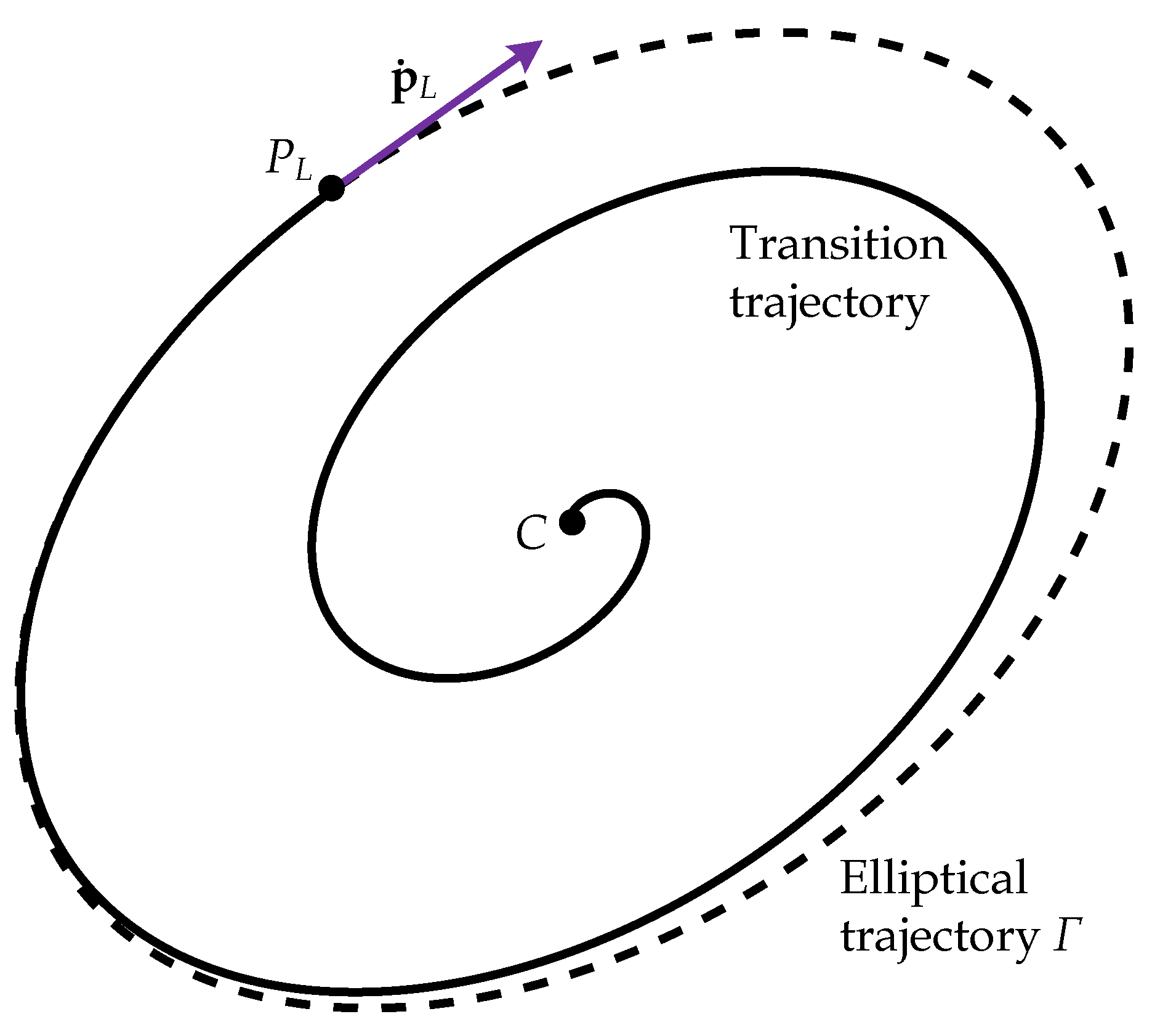
1.2. CSPRs for Throwing Motions

Dynamic trajectory planning allows us to overcome the workspace limitations of CSPRs. However, for tasks where a robot must work across large areas, the motion is still limited by the size of the robot’s architecture, even if dynamic trajectories are used; such motions can then be combined with launch motions to further increase the workspace. Indeed, launch motions allow a robot to complete work tasks over vast areas and may thus provide greater application possibilities for CSPRs; for example, an ideal application would be robotic waste handling [34], where objects may be picked in a point-to-point motion and thrown in distant bins without risk of damaging them or strict position requirements. CSPRs capable of launching objects could also be used for entertainment purposes such as juggling [35] or throwing a ball towards a human player.

The application of robots for casting operations, where a gripper is detached dynamically from the rest of the robot architecture while a tether facilitates control of the gripper mid-flight, was considered in previous works; for instance, Fagiolini et al. [36] designed a manipulator capable of grasping objects at long distances by detaching a gripper from a serial arm. The proposed application of this system was in planetary exploration missions in order to reach objects over rugged terrain; the motion is divided into a start up stage, a stage where the target is reached, and a return stage. Arisumi et al. [37] designed a manipulator system that can be used for launch motions, where a penetrator is thrown towards a desired position by the inertial force generated by the rotation of the manipulator arm around a horizontal axis. Later, a prototype robot for shooting operations, which imitates the behavior of chameleons while preying on insects, was proposed in [38].

Casting robots can quickly capture distant targets with high efficiency—but they can only catch light-weight, small objects; thus, their application range is limited; thus, some authors considered instead purely ballistic motions, where the launched object is released from a robot without a tether. Thus, a throwable workspace can be defined [39] for a robot as the set of objects that can be reached by throwing beyond the reachable workspace, by optimizing the launch angle and speed. Zeng et al. [40] described a mixed method based on both a deep-learning framework and a physical model of the ballistic launch for controlling a serial robot launching objects into selected boxes. Hassan et al. [41,42] presented a control law for throwing motions using a Delta-like parallel robot with the EE having constant orientation. Frank et al. [43] proposed a new object transportation method based on throwing operations, in which the object is thrown towards a distant target and captured at that target; later [44], an application was proposed for automated production systems with the launch and capture of cylindrical objects. At the same time, a new robot system was proposed based on this method and the feasibility of this concept was verified. However, the choice of the launch trajectory was limited by the throwing device. In recent works, throwing motions were also performed by a soft serial manipulator based on flexible chambers [45]. A global survey of methods (including throwing and catching) to manipulate objects without direct constraining through robots can be found in [46].

1.3. A Novel Concept of a CSPR for Throwing Operations

Based on concepts from [43], combined with the intrinsic advantages of CSPRs (such as a relatively high flexibility in trajectory design), we propose the use of CSPRs to perform launch motions, so that an object can reach target points far away from the robot base. In previous works [47,48], we analyzed a case in which the robot starts from a stationary state, slowly reaches a target elliptical motion through a transition trajectory (with gradually increasing amplitudes), and then completes the launch while moving along the elliptical trajectory. This choice in the trajectory design phase allowed us to directly reuse previous results on dynamically-feasible motions [24,31]; moreover, the trajectories thus found are general and flexible enough for application. The schematic of such a launch motion is shown in Figure 1, where point C is both the starting point and the center of ellipse $\Gamma$, $P_L$ is the launch point and ${\dot{\mathbf{p}}}_L$ is the velocity at $P_L$.

Having analyzed periodic motions for throwing in previous works, we now turn our attention towards point-to-point motions, which are often required in practice. We thus aim to define motions that pass through a series of target points $T_i$, reaching zero velocity at each point; this way, an object may be picked up at a target point, $T_j$, to be later released with a launch motion while the EE moves between two successive target points $T_k-T_{k+1}$ (with $k\ge j$). While the EE keeps moving, the launched object reaches its final destination at point $P_T$ while following a purely ballistic motion. For this task, we propose using Bézier curves, which combine flexibility (in terms of the trajectories that can be defined) with a relatively simple analytical definition, and find the conditions for the EE to pass through all points $T_i$ and to launch the object at the correct point $P_L$ (with the required velocity to reach $P_T$). Since the cable tensions are required to be positive at all times, we also find constraints that guarantee the feasibility of the motion; these constraints correspond to simple algebraic inequalities, which can be verified in milliseconds on any modern PC for robot control.

An example of point-to-point launch motion is shown in Figure 2, where $T_1$ and $T_5$ are the initial and final points; the launch occurs in the final segment $T_4-T_5$. Point-to-point trajectory planning is usually more flexible, so we can choose different intermediate points $T_i$ (to avoid obstacles in the workspace, for example) and finally reach the target point.

Besides the kinematic constraint of passing through the targets ($T_i$ and $P_T$) and the dynamic constraint on the cable tensions, other requirements need to be set for the motion to be feasible in practice. Throughout the trajectory, the motion control needs to be reasonably accurate, since small errors in the launch position and velocity could be amplified during the free-flight phase. For these reasons, we applied the architecture first studied in [11], which allows us to control the position of the launched mass with only three actuators; this way, we obtain a simple, fully-actuated design that only requires as many actuators as DoFs. The orientation of the launched object, which is modeled as a point mass, can be disregarded in practical cases, but it is necessary to keep a constant orientation of the EE which carries the object itself; this is guaranteed by the design of our robot with no need for extra actuators. We also verified the robustness of the design using sensitivity indexes with respect to unavoidable control errors.

Finally, we verified our theoretical results by performing simulations, in which we compared our trajectory design approach with alternatives found in the literature, and found that it is both effective and simple to implement. We also present our first prototype of a CSPR for launch motions, which was designed both to demonstrate the general concept and to understand the advantages and limitations of our approach in experimental practice.

The structure of this paper is as follows: Section 2 describes the spatial, six-cable, 3-DoF CSPR with pairwise-parallel cables considered in this work and establishes its dynamic model. Section 3 presents point-to-point trajectories and an analytical method for verifying their feasibility. Section 4 studies launch trajectories for the CSPR under exam, based on the point-to-point trajectories from Section 3. Section 5 presents results from numerical simulations and experimental tests, which verify our method. In Section 6, we review the results observed in our tests and discuss the advantages and limitations of our approach. Finally, Section 7 summarizes the results in this paper and proposes directions for future work.

2. Design, Kinematic and Dynamic Model

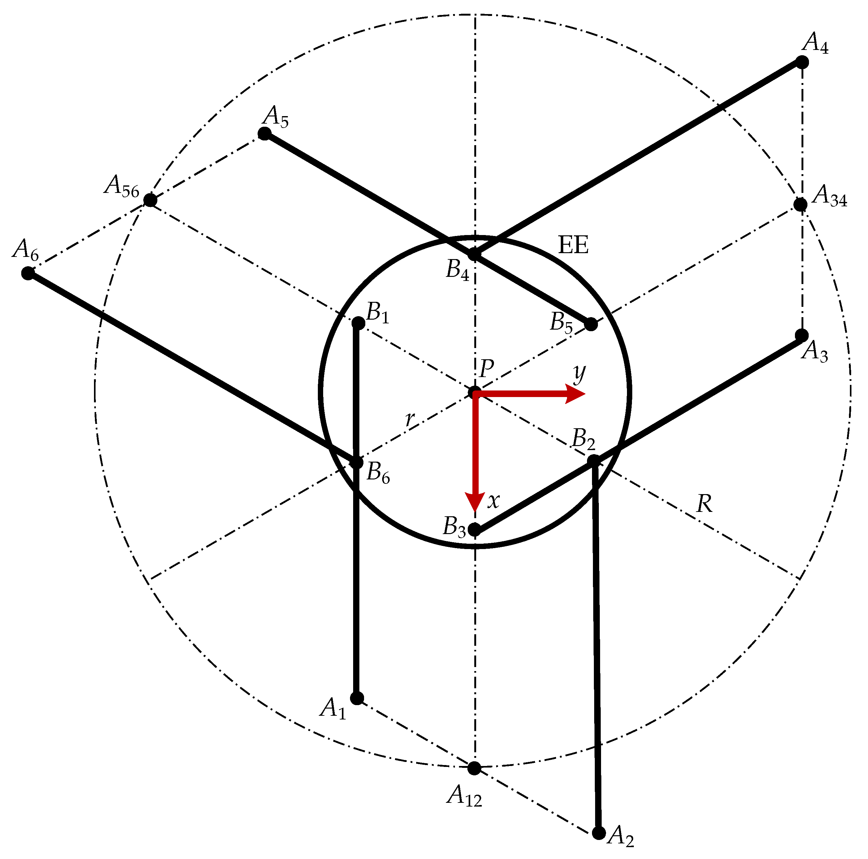
2.1. Robot Architecture

The schematic of our CSPR is shown in Figure 3. The fixed cable exit points $A_i$’s $(i=1,\dots ,6)$ all lie on the same horizontal plane. The cables are connected to the EE at points $B_i(i=1,\dots ,6)$. The cables are pairwise parallel to each other, defining the three cable pairs 1–2, 3–4 and 5–6; each pair is controlled by a motorized winch, and the two points $A_i$ and $A_j$ in a pair are at the same distance from the winch. This way, a winch rotation changes the lengths of the two cables in the corresponding pair by equal amounts. A reference (fixed) Cartesian coordinate frame $OXYZ$ and a frame $Pxyz$ (moving with the EE) are defined in Figure 4; P coincides with the Center of Mass (CoM) of the EE. We also define vectors ${\mathbf{a}}_i=A_i-O$ and ${\mathbf{b}}_i=P-B_i$. The EE position is provided by vector $\mathbf{p}=P-O={\left[x,y,z\right]}^T$.

2.2. Kinematic and Dynamic Model

The inverse kinematic equations for a 6-DoF, six-cable CSPR can be written as follows:

$${\rho }_i=\sqrt{{(\mathbf{p}+\mathbf{Q}{\mathbf{b}}_i-{\mathbf{a}}_i)}^T(\mathbf{p}+\mathbf{Q}{\mathbf{b}}_i-{\mathbf{a}}_i)},i=1,\dots ,6$$

(1)

($\mathbf{Q}$ is the rotation matrix from $Pxyz$ to $OXYZ$, and ${\rho }_i$ is the length of the i-th cable, from $A_i$ to $B_i$). The unit vectors ${\mathbf{e}}_i$, along the i-th cable and oriented towards the EE, are as follows:

$${\mathbf{e}}_i=\frac{\mathbf{p}+\mathbf{Q}{\mathbf{b}}_i-{\mathbf{a}}_i}{{\rho }_i}$$

(2)

Neglecting the elasticity and the mass of the cables, the dynamic model is found as follows:

$$\begin{array}{cc}\hfill \sum _{i=1}^6(-{\tau }_i{\mathbf{e}}_i)+m\mathbf{g}& =m\ddot{\mathbf{p}}\hfill \\ \hfill \sum _{i=1}^6\left[\left(\mathbf{Q}{\mathbf{b}}_i\right)\times (-{\tau }_i{\mathbf{e}}_i)\right]& =\mathbf{Q}(\mathbf{I}\dot{\mathit{\omega }}+\mathit{\omega }\times \mathbf{I}\mathit{\omega })\hfill \end{array}$$

(3)

where m is the mass of the EE, $\mathbf{I}$ is its inertia tensor, $\mathit{\omega }$ and $\dot{\mathit{\omega }}$ are, respectively, its angular velocity and acceleration (in frame $Pxyz$), and $\mathbf{g}={\left[0,0,-g\right]}^T$ is the gravity vector (with $g=9.80665$ m/s²); the tension in the i-th cable is ${\tau }_i$. Then, Equation (3) can be written as follows:

$$\mathbf{M}\mathit{\tau }=\gamma$$

(4)

where

$$\mathbf{M}=\left[\begin{array}{ccc}{\mathbf{e}}_1& \dots & {\mathbf{e}}_6\\ {\mathbf{e}}_1\times \mathbf{Q}{\mathbf{b}}_1& \dots & {\mathbf{e}}_6\times \mathbf{Q}{\mathbf{b}}_6\end{array}\right],\gamma =\left[\begin{array}{c}m\mathbf{g}-m\ddot{\mathbf{p}}\\ \mathbf{Q}(\mathbf{I}\dot{\mathit{\omega }}+\mathit{\omega }\times \mathbf{I}\mathit{\omega })\end{array}\right]$$

(5)

while $\mathit{\tau }={[{\tau }_1,\dots ,{\tau }_6]}^T$ is the vector of cable tensions. From Equation (4), the cable tensions are

$$\mathit{\tau }={\mathbf{M}}^{-1}\gamma$$

(6)

The condition for dynamic feasibility is then $\mathit{\tau }⪰0$, where ⪰ is the element-wise inequality; in other words, it must hold that ${\tau }_i\ge 0$ for all i (at each instant during the motion).

As found in [11,49], the kinematic and dynamic analyses are much simpler under some assumptions in the design. Consider the case where the cable attachment points are placed on the fixed frame and on the EE such that $A_1-A_2=B_1-B_2$ at an initial pose. Additionally, cables 1 and 2 have the same length at all times (see Figure 4); this is achieved by controlling both cables with one winch (see Section 2.1). Analogous relationships are defined for cable pairs 3–4 and 5–6 and for the corresponding $A_i$’s and $B_i$’s. With this design, each cable pair defines a parallelogram. Taken together, the pairs constrain all EE rotations [9,19]; thus, the robot is purely translational, with 3 DoFs (along the X-, Y- and Z-axes).

In a further specialization, P is at the intersection of segments $\overline{B_1{B}_2}$, $\overline{B_3{B}_4}$, and $\overline{B_5{B}_6}$. It has been proven [11] that the CSPR with finite-size EE under examination is then dynamically equivalent to a simpler, 3-DoF CSPR with point-mass EE (with cable exit points $A_{12}$, $A_{34}$, and $A_{56}$ on $\overline{A_1{A}_2}$, $\overline{A_3{A}_4}$, and $\overline{A_5{A}_6}$, respectively): the SEW is the same for both robots, and the feasibility condition is simply that the sums of the cable tensions in each pair must be positive. Additionally, if P is at the midpoint of $\overline{A_1{A}_2}$, $\overline{A_3{A}_4}$, and $\overline{A_5{A}_6}$ (see Figure 3), then ${\tau }_1={\tau }_2$, ${\tau }_3={\tau }_4$ and ${\tau }_5={\tau }_6$, which is desirable so that the forces on a winch balance each other out. Given its simplicity of design and analysis, this final architecture (with ${\mathbf{b}}_1=-{\mathbf{b}}_2$, ${\mathbf{b}}_3=-{\mathbf{b}}_4$ and ${\mathbf{b}}_5=-{\mathbf{b}}_6$) will be used in the rest of this work and in the prototype.

2.3. Jacobian Matrix and Sensitivity Indexes

The Jacobian of a generic six-cable CSPR can be written as $\mathbf{J}=\mathbf{J}(\mathbf{p},\mathbf{Q})={\mathbf{M}}^{-T}$. The first-order kinematics equation is then $\mathbf{J}\dot{\mathit{\rho }}={\left[{\dot{\mathbf{p}}}^T,{\mathit{\omega }}^T\right]}^T$, where $\dot{\mathit{\rho }}={[{\dot{\rho }}_1,\dots ,{\dot{\rho }}_6]}^T$ is the vector of cable velocities; these equations are necessary for the motion control of our prototype.

From $\mathbf{J}$, we derive the error sensitivities; these indexes measure the robustness of the pose to unavoidable errors in the input joint coordinates (here, a vector $d\mathit{\rho }={\left[d{\rho }_1,\dots ,d{\rho }_6\right]}^T$ of errors $d{\rho }_i$ in the lengths ${\rho }_i$). These can be due to assembly tolerances or to the tracking accuracy of the control system. Several definitions of the sensitivity have been proposed [50,51]; a recurring issue is that the pose has elements in different units, namely the position error $d\mathbf{p}$, with units of length, and the orientation error $d\mathit{\varphi }$, with angular units. Thus, using $\mathbf{J}$ to define the sensitivities implies mixing dimensionally inconsistent values [52,53]. Several alternatives have been proposed [54], but a standard approach has yet to be defined.

We use the definitions provided in [49], which avoid such inconsistencies and can be computed quickly. We separate $\mathbf{J}={\left[{\mathbf{J}}_p^T,{\mathbf{J}}_r^T\right]}^T$ into $3\times 6$ matrices ${\mathbf{J}}_p$ and ${\mathbf{J}}_r$. Remarkably, for the design in Figure 3, $\mathbf{M}$ can be inverted analytically; thus, ${\mathbf{J}}_p$ and ${\mathbf{J}}_r$ can be written in closed form (see Appendix A). We can now define the sensitivities as functions of the pose:

$${\sigma }_p(\mathbf{p},\mathbf{Q})=\underset{{\parallel d\mathit{\rho }\parallel }_{\infty }=1}{max}{\parallel d\mathbf{p}\parallel }_2={\parallel {\mathbf{J}}_p\parallel }_{\infty ,2},{\sigma }_r(\mathbf{p},\mathbf{Q})=\underset{{\parallel d\mathit{\rho }\parallel }_{\infty }=1}{max}{\parallel d\mathit{\varphi }\parallel }_2={\parallel {\mathbf{J}}_r\parallel }_{\infty ,2}$$

(7)

where ${\parallel •\parallel }_q$ ($q\ge 1$) is the q-norm of vector $\left(•\right)$, and ${\parallel \circ \parallel }_{q,s}$ is the norm of matrix $\left(\circ \right)$ induced by the q- and s-vector norms [55]. These sensitivities provide upper bounds to the pose errors; if the errors are all within a range $d{\rho }_i\in \left[-d{\rho }_{max},d{\rho }_{max}\right]$, then ${\parallel d\mathit{\varphi }\parallel }_2$ (the rotation angle of the EE) is at most ${\sigma }_{r}d{\rho }_{max}$, and a similar relationship holds for the maximum position error ${\parallel d\mathbf{p}\parallel }_2$. These concepts will be used later to verify the design of the prototype.

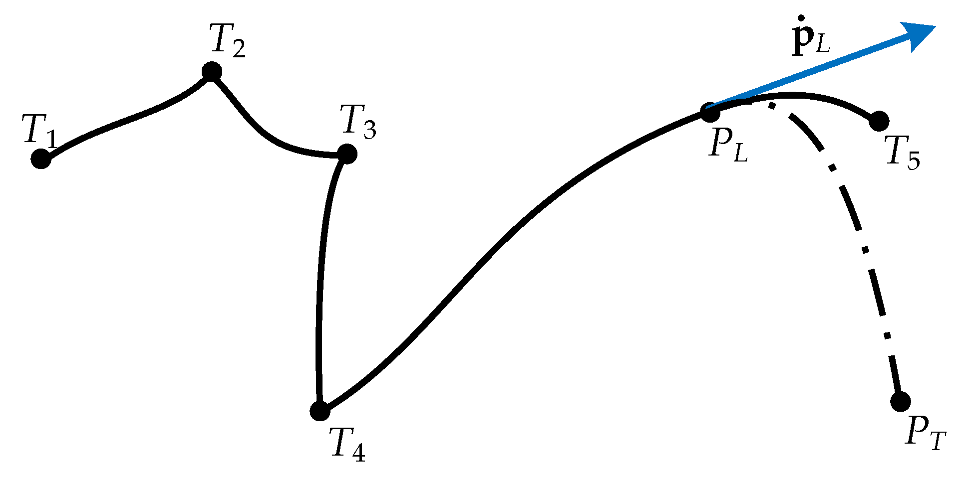
3. Point-to-Point Trajectory Planning

3.1. Parametric Equation of the Trajectory

In designing the trajectory, we require the EE to visit N given intermediate target points $T_i$ sequentially, each at a desired time $t_{0,i}\left(i=1,\dots ,N\right)$, in a point-to-point motion (with zero velocity $\dot{\mathbf{p}}$ at each point $T_i$); the points $T_i$ may in general be outside the SEW.

We divide the global trajectory $\mathbf{p}=\mathbf{p}\left(t\right)$ into a number of segments $\mathbf{p}={\mathbf{p}}_i\left(t_i^{\prime }\right)$, $t_i^{\prime }\in \left[0,\Delta t_i\right]$, where $t_i^{\prime }=t-t_{0,i}$ is the time elapsed since the beginning of the ith trajectory segment (at time $t_{0,i}$) and $\Delta t_i=t_{0,i+1}-t_{0,i}$ is the segment duration. To maintain the continuity of the motion across consecutive segments, the kinematic constraints on the trajectory are given as follows:

$$\left\{\begin{array}{llll}{\mathbf{p}}_i\left(0\right)& ={\mathbf{t}}_i,& {\mathbf{p}}_i(\Delta t_i)& ={\mathbf{t}}_{i+1}\\ {\dot{\mathbf{p}}}_i\left(0\right)& =0,& {\dot{\mathbf{p}}}_i(\Delta t_i)& =0\\ {\ddot{\mathbf{p}}}_i(\Delta t_i)& ={\ddot{\mathbf{p}}}_{i+1}\left(0\right)& \hfill & & \hfill \end{array}\right.$$

(8)

where ${\mathbf{t}}_i=T_i-O={\left[x_i,y_i,z_i\right]}^T$ is the position vector of the ith target point to be visited, and ${\dot{\mathbf{p}}}_i$ and ${\ddot{\mathbf{p}}}_i$ are, respectively, the velocity and acceleration of point P along the ith segment.

For simplicity, we choose to define each trajectory segment as a Bézier curve of the second order [56]. A similar concept was also advanced in [57], using second-order Bézier curves as a basis for planning dynamically feasible trajectories for a simpler three-cable robot that is dynamically equivalent to the one presented here; later, in [58], this concept was extended to B-splines (a generalization of Bézier curves) of the fifth order, which were applied to an overconstrained, 12-cable robot with translational motion with parallelogram actuation. We also refer to [59], which discusses a cable robot designed for artistic and entertainment purposes, where the trajectories are described by third-order Bézier curves, but without considering dynamic feasibility.

The shape of a Bézier curve is determined by its control points $T_i$. The resulting trajectory is thus simple in its definition, yet flexible. If the start and end control points of the curve are given, the intermediate control points can be freely selected. The parametric equation of the Bézier curve trajectory segment can be written as follows:

$${\mathbf{p}}_i\left(t_i^{\prime }\right)={(1-s_i)}^2{\mathbf{t}}_i+2s_i(1-s_i){\mathbf{t}}_{m,i}+s_i^2{\mathbf{t}}_{i+1}$$

(9)

where $s_i=s_i\left(t_i^{\prime }\right)\in [0,1]$ is a suitable function of time $t_i^{\prime }$ (continuous up to the second derivative) and ${\mathbf{t}}_{m,i}=T_{m,i}-O$ is the position vector of the intermediate control point $T_{m,i}$ for the ith trajectory segment. We now calculate the first and second derivatives of Equation (9) with respect to time, obtaining (respectively)

$${\dot{\mathbf{p}}}_i\left(t_i^{\prime }\right)=2{\dot{s}}_i\left[(s_i-1){\mathbf{t}}_i+(1-2s_i){\mathbf{t}}_{m,i}+s_i{\mathbf{t}}_{i+1}\right]$$

(10)

and

$${\ddot{\mathbf{p}}}_i\left(t_i^{\prime }\right)=2\left[\left({\dot{s}}_i^2+s_i{\ddot{s}}_i-{\ddot{s}}_i\right){\mathbf{t}}_i+\left({\ddot{s}}_i-2{\dot{s}}_i^2-2s_i{\ddot{s}}_i\right){\mathbf{t}}_{m,i}+({\dot{s}}_i^2+s_i{\ddot{s}}_i){\mathbf{t}}_{i+1}\right]$$

(11)

Substituting Equations (9)–(11) into Equation (8), the constraints on $s_i\left(t_i^{\prime }\right)$ are found as follows:

$$\{\begin{array}{}\mathrm{(12a)}& s_i\left(0\right)=0, s_i(\Delta t_i)=1\mathrm{(12b)}& {\dot{s}}_i\left(0\right)=0, {\dot{s}}_i(\Delta t_i)=0\mathrm{(12c)}& ({\mathbf{t}}_{i+1}-{\mathbf{t}}_{m,i}){\ddot{s}}_i(\Delta t_i)=({\mathbf{t}}_{m,i+1}-{\mathbf{t}}_{i+1}){\ddot{s}}_i\left(0\right)\end{array}$$

Several motion laws known from the literature [60] could be chosen that respect the constraints in Equations (12b) and (12c). One of the simplest choices for function $s_i\left(t_i^{\prime }\right)$ is

$$s_i\left(t_i^{\prime }\right)=-\frac{1}{2}cos\left(\frac{\pi t_i^{\prime }}{\Delta t_i}\right)+\frac{1}{2}$$

(13)

(compare with [57], where the path variable was defined through a differential equation). The first and second derivatives of $s_i\left(t_i^{\prime }\right)$ are then, respectively,

$${\dot{s}}_i\left(t_i^{\prime }\right)=\frac{\pi }{2\Delta t_i}sin\left(\frac{\pi t_i^{\prime }}{\Delta t_i}\right),{\ddot{s}}_i\left(t_i^{\prime }\right)=\frac{{\pi }^2}{2\Delta t_i^2}cos\left(\frac{\pi t_i^{\prime }}{\Delta t_i}\right)$$

(14)

Substituting Equation (14) into Equation (12c), the condition for the continuity of acceleration is as follows:

$${\mathbf{t}}_{m,i+1}={\mathbf{t}}_{i+1}+\left({\mathbf{t}}_{m,i}-{\mathbf{t}}_{i+1}\right){\left(\frac{\Delta t_{i+1}}{\Delta t_i}\right)}^2$$

(15)

The position vectors ${\mathbf{t}}_i$ are known constraints for the trajectory design, as are the times $\Delta t_i$ to move from one target point to the next one. Thus, the intermediate control points can be found in an iterative fashion: ${\mathbf{t}}_{m,1}$ (for the first segment) can be chosen arbitrarily, while ${\mathbf{t}}_{m,2}$ is found from ${\mathbf{t}}_{m,1}$ and ${\mathbf{t}}_2$; then, from ${\mathbf{t}}_{m,2}$, we find in turn ${\mathbf{t}}_{m,3}$ and so on.

3.2. Cable Tension Constraints

For convenience, we use the following shorthands:

$$c_{\theta }=cos\left(\frac{\pi t_i^{\prime }}{\Delta t_i}\right),s_{\theta }=sin\left(\frac{\pi t_i^{\prime }}{\Delta t_i}\right)$$

(16)

Substituting Equations (13) and (14) into Equations (9) and (11), we have

$${\mathbf{p}}_i\left(t_i^{\prime }\right)=\frac{1}{4}\left[({\mathbf{t}}_i-2{\mathbf{t}}_{m,i}+{\mathbf{t}}_{i+1})c_{\theta }^2+2({\mathbf{t}}_i-{\mathbf{t}}_{i+1})c_{\theta }+({\mathbf{t}}_i+2{\mathbf{t}}_{m,i}+{\mathbf{t}}_{i+1})\right]$$

(17)

and

$${\ddot{\mathbf{p}}}_i\left(t_i^{\prime }\right)=\frac{{\pi }^2}{2{(\Delta t_i)}^2}\left[2(-{\mathbf{t}}_i+2{\mathbf{t}}_{m,i}-{\mathbf{t}}_{i+1})c_{\theta }^2+(-{\mathbf{t}}_i+{\mathbf{t}}_{i+1})c_{\theta }+({\mathbf{t}}_i-2{\mathbf{t}}_{m,i}+{\mathbf{t}}_{i+1})\right]$$

(18)

We now substitute Equations (15), (17) and (18) into Equation (6) for a generic six-cable suspended robot. We also set the orientation $\mathbf{Q}$ of the EE as constant; thus, the angular velocity $\mathit{\omega }$ and acceleration $\dot{\mathit{\omega }}$ are both zero. We then find after simplification that the conditions for positive cable tensions are always defined by third-order polynomials, such as

$${\mu }_j\left(t_i^{\prime }\right)=f_{3j}{c}_{\theta }^3+f_{2j}{c}_{\theta }^2+f_{1j}{c}_{\theta }+f_{0j}>0,j=1,\dots ,6$$

(19)

in which the ${\mu }_j=m{\tau }_j/{\rho }_j$ are auxiliary quantities with the same sign as the actual cable tensions ${\tau }_j$ (since both the EE mass m and the cable lengths ${\rho }_j$ are always positive) while being easier to compute. The general expressions for coefficients $f_{kj}$ in Equation (19), which depend on the architecture parameters, are not reported here for brevity.

The time derivative of Equation (19) is

$$\frac{d{\mu }_j\left(t_i^{\prime }\right)}{d{t}_i^{\prime }}=\frac{\partial {\mu }_j}{\partial c_{\theta }}\frac{d{c}_{\theta }}{d{t}_i^{\prime }}=\underset{={\zeta }_j\left(c_{\theta }\right)}{\underbrace{\left(3f_{3j}{c}_{\theta }^2+2f_{2j}{c}_{\theta }+f_{1j}\right)}}\left(-s_{\theta }\frac{\pi }{\Delta t_i}\right)$$

(20)

Since $t_i^{\prime }\in \left[0,\Delta t_i\right]$, the second term of the right-hand side does not change sign; therefore, the sign of Equation (20) only depends on the first term ${\zeta }_j$, which is a quadratic function in the variable $c_{\theta }$. Setting ${\zeta }_j=0$, the discriminant of the resulting second-order equation is as follows:

$$\Delta =4f_{2j}^2-12f_{3j}{f}_{1j}$$

(21)

When verifying feasibility for the jth cable, we can then have the following cases.

• When $\Delta <0$, Equation (20) is either always positive or always negative; thus, ${\mu }_j$ is a monotonic function. It is then sufficient to verify that Equation (19) is satisfied at the extremes of the trajectory segment:

  $${\mu }_j\left(0\right)>0,{\mu }_j(\Delta t_i)>0$$

  (22)
• When $\Delta =0$, Equation (20) has two coincident roots, namely

  $$n_1=n_2=\frac{-f_{2i}}{3f_{3i}}$$

  (23)
  Again, ${\zeta }_j$ always has the same sign, except at the repeated root (where it becomes zero): this corresponds to an inflection point for ${\mu }_j$, which is otherwise monotonic. Therefore, we fall back to case 1 above, and it is sufficient to verify that Equation (22) holds.
• When $\Delta >0$, ${\zeta }_j$ has two distinct roots, namely

  $$n_1=\frac{-2f_{2i}+\sqrt{\Delta }}{6f_{3i}},n_2=\frac{-2f_{2i}-\sqrt{\Delta }}{6f_{3i}}$$

  (24)

  where one root corresponds to a local minimum of ${\mu }_j$ and the other to a maximum. If ${\mu }_j$ is positive at these two local extrema, at the beginning of the trajectory segment, and at its end, then Equation (19) is always satisfied. The following conditions then need to be verified:

  $${\mu }_j\left(0\right)>0,{\mu }_j(\Delta t_i)>0,max[{\mu }_j\left(n_1\right),{\mu }_j\left(n_2\right)]>0$$

  (25)

Notice that the roots $n_1$ and $n_2$ can be directly calculated (in case 3) from the trajectory parameters. We only consider roots in the interval $[-1,1]$, as $c_{\theta }$ is the cosine of a real angle.

Equations (22) and (25), then, are functions in only one variable $\left(\Delta t_i\right)$, which is known in the trajectory design phase. We can then easily verify the feasibility through an analytical procedure rather than verifying that cable tensions are positive at each time step. Moreover, if the desired trajectory is found to be unfeasible, it is also easier to find values for $\Delta t_i$ (by trial and error) that ensure feasibility. Several Bézier curve segments can then be combined in series, while ensuring both feasibility and continuity up to the acceleration. Our method is similar to the one in [57] but leads to conditions that are easier to verify and does not require the intermediate control point ${\mathbf{t}}_{m,i}$ to be in the SEW.

4. Launch Trajectory Planning

We now consider the motion of the object launched from the EE, assuming that the EE starts moving from rest, reaches the launch point $P_L$, and then launches an object (modeled as a point mass) which will pass through a target point $P_T$. In our prototype, this is achieved by opening a gripper on the EE while the latter moves at velocity ${\dot{\mathbf{p}}}_L$.

After launch, the object moves under the effect of gravity. Like most authors [35,36,37,38], we assume that air resistance can be neglected; otherwise, the differential equations for the launch motion cannot be solved in closed form. Disregarding air drag with respect to the gravitational force is also reasonable if the launched object is relatively small and dense.

The free-flight motion of the launched object is then a ballistic (parabolic) trajectory in a vertical plane, given by

$$\begin{array}{}\mathrm{(26a)}& {\mathbf{p}}_b\left(t\right)=\frac{1}{2}\mathbf{g}{\left(t-t_L\right)}^2+{\dot{\mathbf{p}}}_L\left(t-t_L\right)+{\mathbf{p}}_L\mathrm{(26b)}& {\dot{\mathbf{p}}}_b\left(t\right)=\hspace{1em}\mathbf{g}\left(t-t_L\right)+{\dot{\mathbf{p}}}_L\end{array}$$

Here, $t_L$ is the launch instant, which occurs during the i-th segment of the trajectory; the time since the start of the corresponding segment is $t_{iL}^{\prime }=t_L-t_{0,i}\in [0,\Delta t_i]$.

In a practical case, the target point position ${\mathbf{p}}_T$ is known, and so is the velocity ${\dot{\mathbf{p}}}_T$ at the target. For instance, if $P_T$ corresponds to an opening through which the object is to pass (to be collected in a bin), ${\dot{\mathbf{p}}}_T$ should be normal to the opening, to increase the likelihood of a successful throw; the magnitude of ${\dot{\mathbf{p}}}_T$ is then chosen from safety and speed considerations.

Setting ${\mathbf{p}}_b={\mathbf{p}}_T$ and ${\dot{\mathbf{p}}}_b={\dot{\mathbf{p}}}_T$ from Equations (26a) and (26b) fully defines the parabolic trajectory. On this parabola, we pick a launch point $P_L$: this can be chosen either arbitrarily or through optimization, by searching the position of $P_L$ along the parabola that minimizes objective functions, such as the total energy and time requested for the launch [47]. The speed at the launch point is then found by solving Equation (26b) for the unknown ${\dot{\mathbf{p}}}_L$.

With these assumptions, our goal is to design a trajectory segment in the form of Equation (9) that passes through the launch point ${\mathbf{p}}_L={[x_L,y_L,z_L]}^T$ at a set speed ${\dot{\mathbf{p}}}_L={\left[{\dot{x}}_L,{\dot{y}}_L,{\dot{z}}_L\right]}^T$. We assume that the position of the initial point $T_i$ of the trajectory segment is known. From Equation (17), the position at the launch point can be obtained as follows:

$${\mathbf{p}}_L=\frac{1}{4}\left[({\mathbf{t}}_i-2{\mathbf{t}}_{m,i}+{\mathbf{t}}_{i+1})c_{\theta L}^2+2({\mathbf{t}}_i-{\mathbf{t}}_{i+1})c_{\theta L}+({\mathbf{t}}_i+2{\mathbf{t}}_{m,i}+{\mathbf{t}}_{i+1})\right]$$

(27)

while, from Equations (10), (13) and (14), the launch velocity is

$${\dot{\mathbf{p}}}_L=-\frac{\pi }{2\Delta t_i}\left[({\mathbf{t}}_i-2{\mathbf{t}}_{m,i}+{\mathbf{t}}_{i+1})c_{\theta L}+({\mathbf{t}}_i-{\mathbf{t}}_{i+1})\right]s_{\theta L}$$

(28)

using the shorthands $c_{\theta L}=cos\left(\frac{\pi t_{iL}^{\prime }}{\Delta t_i}\right)$ and $s_{\theta L}=sin\left(\frac{\pi t_{iL}^{\prime }}{\Delta t_i}\right)$.

In our case, we want the launched object to pass through $P_T$ at a desired time $t_T$; from this and Equations (26a) and (26b), $t_L$ is easily found, from which we find $t_{iL}^{\prime }$ and then $c_{\theta L}$ and $s_{\theta L}$. The motion time $\Delta t_i$ for the trajectory segment is also known, as discussed in Section 3.1.

We can then solve Equations (27) and (28) for the unknowns ${\mathbf{t}}_{m,i}={[x_{m,i},y_{m,i},z_{m,i}]}^T$ and ${\mathbf{t}}_{i+1}={[x_{i+1},y_{i+1},z_{i+1}]}^T$, whose components are found as

$$\begin{array}{cccc}\hfill x_{m,i}& =\frac{x_i(1+c_{\theta L})-2x_L}{c_{\theta L}-1}\hfill & & -\frac{\Delta t_i{\dot{x}}_L}{\pi s_{\theta L}}\hfill \end{array}$$

(29a)

$$\begin{array}{cccc}\hfill y_{m,i}& =\frac{y_i(1+c_{\theta L})-2y_L}{c_{\theta L}-1}\hfill & & -\frac{\Delta t_i{\dot{y}}_L}{\pi s_{\theta L}}\hfill \end{array}$$

(29b)

$$\begin{array}{cccc}\hfill z_{m,i}& =\frac{z_i(1+c_{\theta L})-2z_L}{c_{\theta L}-1}\hfill & & -\frac{\Delta t_i{\dot{z}}_L}{\pi s_{\theta L}}\hfill \end{array}$$

(29c)

$$\begin{array}{cccc}\hfill \hspace{1em}\hspace{1em}\hspace{1em}\hspace{1em}\hspace{1em}\hspace{1em}{x}_{i+1}& =\frac{x_i{(1+c_{\theta L})}^2-4c_{\theta L}{x}_L}{{(c_{\theta L}-1)}^2}\hfill & & -\frac{2\Delta t_i{\dot{x}}_L(1+c_{\theta L})}{\pi s_{\theta L}(c_{\theta L}-1)}\hfill \end{array}$$

(29d)

$$\begin{array}{cccc}\hfill \hspace{1em}\hspace{1em}\hspace{1em}\hspace{1em}\hspace{1em}\hspace{1em}{y}_{i+1}& =\frac{y_i{(1+c_{\theta L})}^2-4c_{\theta L}{y}_L}{{(c_{\theta L}-1)}^2}\hfill & & -\frac{2\Delta t_i{\dot{y}}_L(1+c_{\theta L})}{\pi s_{\theta L}(c_{\theta L}-1)}\hfill \end{array}$$

(29e)

$$\begin{array}{cccc}\hfill \hspace{1em}\hspace{1em}\hspace{1em}\hspace{1em}\hspace{1em}\hspace{1em}{z}_{i+1}& =\frac{z_i{(1+c_{\theta L})}^2-4c_{\theta L}{z}_L}{{(c_{\theta L}-1)}^2}\hfill & & -\frac{2\Delta t_i{\dot{z}}_L(1+c_{\theta L})}{\pi s_{\theta L}(c_{\theta L}-1)}\hfill \end{array}$$

(29f)

This way, the trajectory segment is fully defined. If this launch trajectory is found to be unfeasible, one can change the time $\Delta t_i$ to reach the final point; a feasible trajectory can then be quickly found by trial and error.

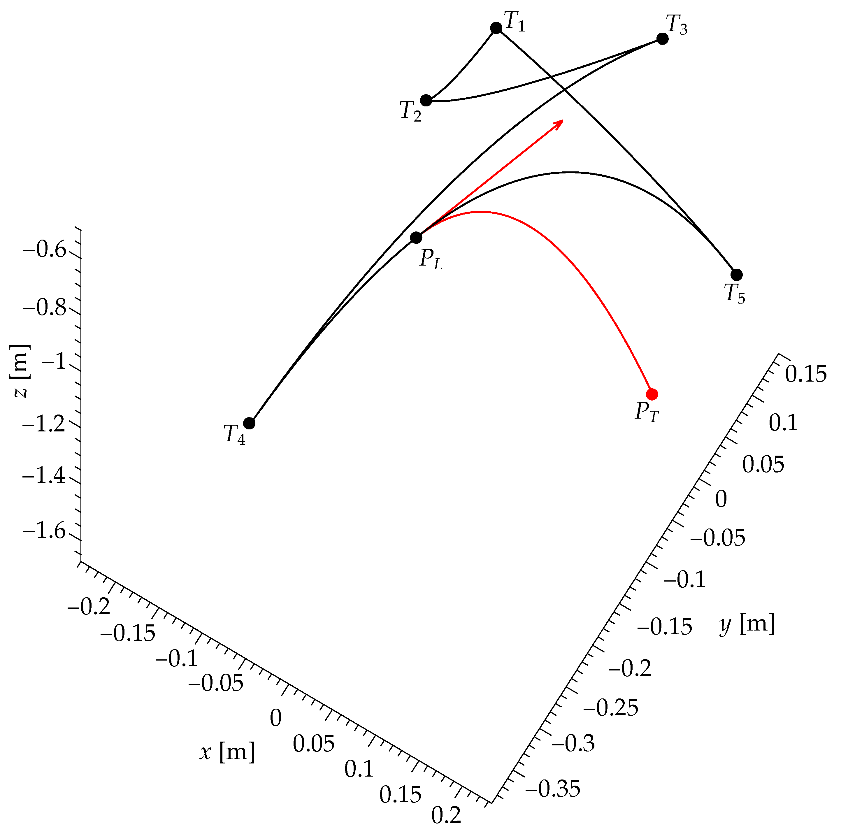
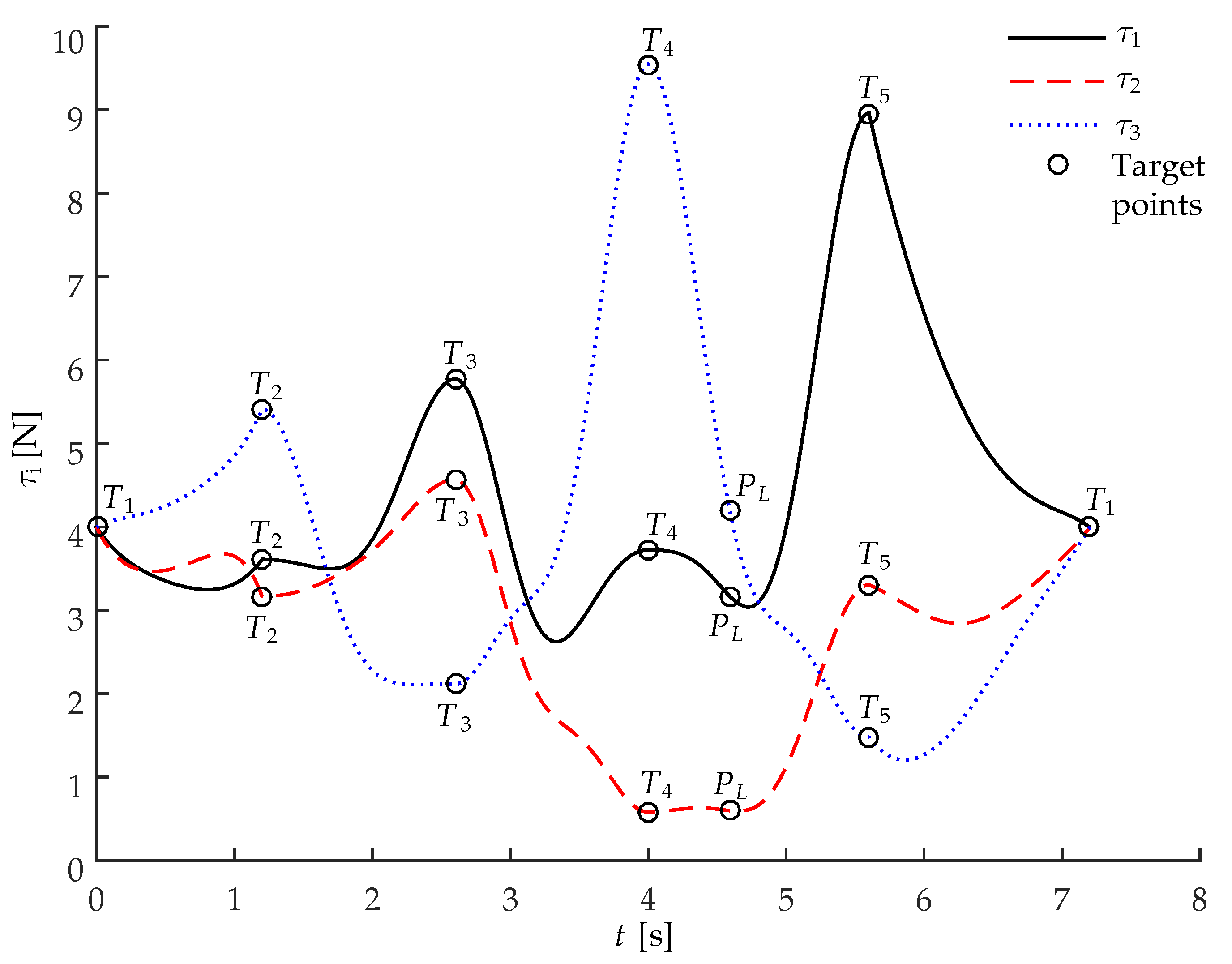
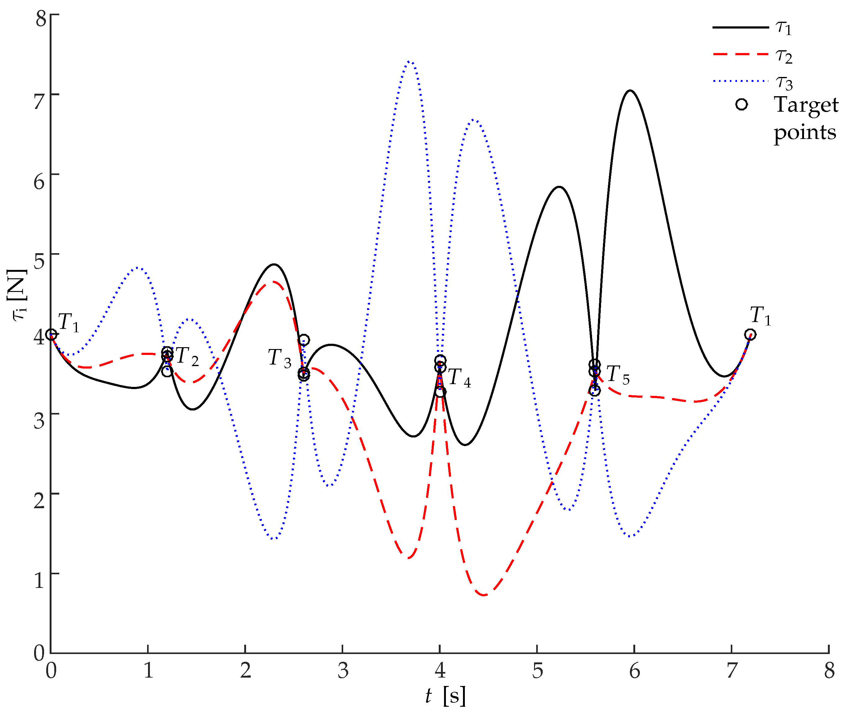
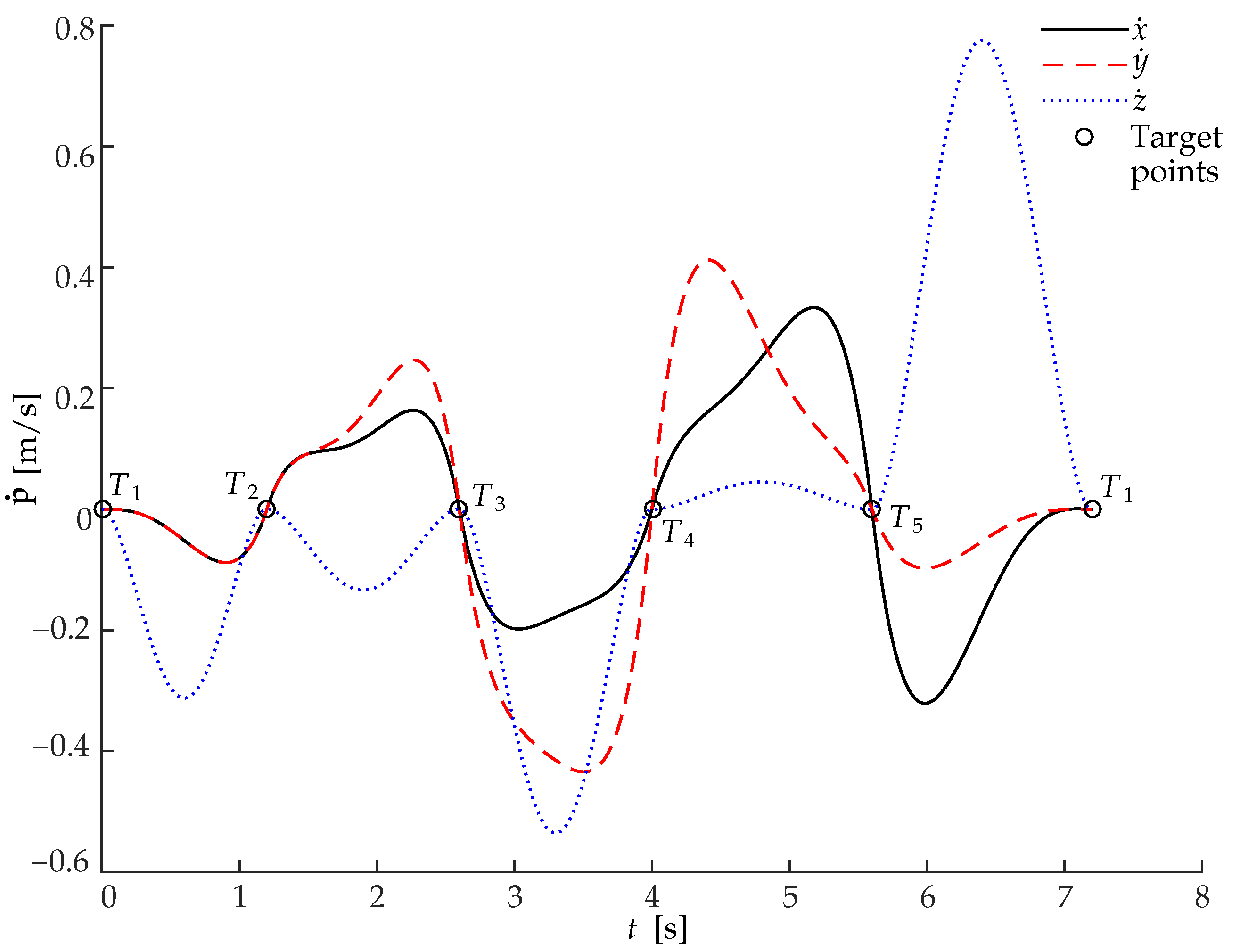
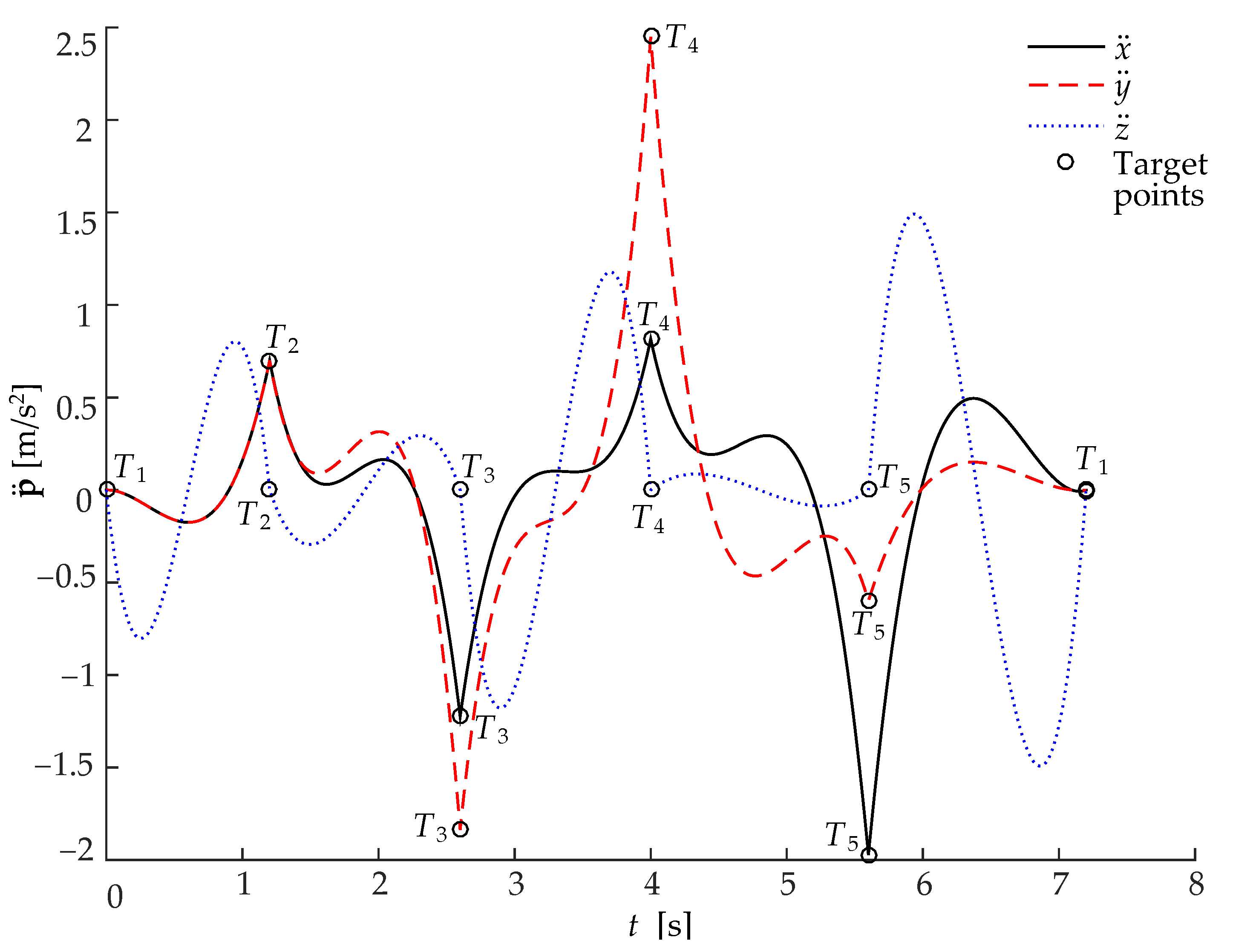
5. Simulations and Experimental Verification

5.1. Final Design

In order to verify the feasibility of the trajectory planning method, we consider a specific robot architecture, whose dimensions are as follows: the midpoints $A_{12}$, $A_{34}$, and $A_{56}$ of the segments $\overline{A_1{A}_2}$, $\overline{A_3{A}_4}$, and $\overline{A_5{A}_6}$ are located at the three vertices of a horizontal equilateral triangle, inscribed in a circle of radius $R=0.35$ m. The mobile cable attachment points are placed on a circle of radius $r=0.09$ on the EE, which has mass $m=1$. Moreover, at the initial position, the EE is placed in such a way that $A_1-A_2=B_1-B_2$, $A_3-A_4=B_3-B_4$, and $A_5-A_6=B_5-B_6$, as discussed in Section 2.2; this ensures purely translational motion by controlling each pair of cables, so they are kept at equal lengths. The final architecture is shown in Figure 5.

The components of vectors ${\mathbf{a}}_i$ are

$$\begin{array}{lll}{\mathbf{a}}_1={\left[R-\frac{r}{2},-\frac{\sqrt{3}r}{2},0\right]}^T,& {\mathbf{a}}_2={\left[R+\frac{r}{2},\frac{\sqrt{3}r}{2},0\right]}^T,& {\mathbf{a}}_3={\left[r-\frac{R}{2},\frac{\sqrt{3}R}{2},0\right]}^T\\ {\mathbf{a}}_4={\left[-r-\frac{R}{2},\frac{\sqrt{3}R}{2},0\right]}^T,& {\mathbf{a}}_5={\left[-\frac{R+r}{2},\frac{\sqrt{3}(r-R)}{2},0\right]}^T,& {\mathbf{a}}_6={\left[\frac{r-R}{2},-\frac{\sqrt{3}(r+R)}{2},0\right]}^T\end{array}$$

(30)

and for vectors ${\mathbf{b}}_i$

$$\begin{array}{lll}{\mathbf{b}}_1=r{\left[-\frac{1}{2},-\frac{\sqrt{3}}{2},0\right]}^T,& {\mathbf{b}}_2=r{\left[\frac{1}{2},\frac{\sqrt{3}}{2},0\right]}^T,& {\mathbf{b}}_3=r{\left[1,0,0\right]}^T\\ {\mathbf{b}}_4=r{\left[-1,0,0\right]}^T,& {\mathbf{b}}_5=r{\left[-\frac{1}{2},\frac{\sqrt{3}}{2},0\right]}^T,& {\mathbf{b}}_6=r{\left[\frac{1}{2},-\frac{\sqrt{3}}{2},0\right]}^T\end{array}$$

(31)

In the following, we present results from simulations performed in MATLAB, to confirm the results of Section 3 and Section 4; in all cases, we disregarded the cable mass and all compliance effects (on the cables and on the rest of the structure). These assumptions are acceptable given the lightweight, high-resistance cables used on the prototype and the low weight of the EE. Since the architecture defined by Equations (30) and (31) falls within the special case considered at the end of Section 2.2, we also applied the simplified results from [11]: this way, a simpler analysis can be performed on a three-cable robot with a point-mass EE, which is kinematically and dynamically equivalent to the actual prototype.

Using the design parameters shown above, we first ran a simple simulation to verify whether the assumption of purely-translational motion used throughout this work is in fact valid, even if the desired motion range is quite large. Given the available motion range of the prototype, we thus required point P to move within a rectangular cuboid W defined by

$$x=[-1m,1m],y=[-1m,1m],z=[-1m,0m]$$

(32)

With the definitions from Section 2.3, we then computed the sensitivities ${\sigma }_p$ and ${\sigma }_r$ from Equation (7), along a rectangular grid of regularly-spaced points within W at a distance of 0.001 m from each other (along the x, y and z axes). The maximum values of the sensitivities (at any of the specified points) are found as follows:

$$\underset{\mathbf{p}\in W}{max}\left\{{\sigma }_p(\mathbf{p},\mathbf{E})\right\}=4.8·{10}^{-3}\frac{\mathrm{mm}}{\mathrm{mm}},\underset{\mathbf{p}\in W}{max}\left\{{\sigma }_r(\mathbf{p},\mathbf{E})\right\}=4.5·{10}^{-5}\frac{\mathrm{rad}}{\mathrm{mm}}$$

(33)

(the orientation $\mathbf{Q}$ is in this case constant and equal to the identity matrix $\mathbf{E}$).

The motors used for the prototype have encoders with an angular resolution of 2048 pulses per revolution, and the cables wrap on pulleys with a radius of $r_p=26.75$ mm: thus, the expected maximum error in the cable lengths is $d{\rho }_{max}=2\pi r_p/2048=0.08$ mm. Then, as noted in Section 3, we have ${\parallel d\mathit{\varphi }\parallel }_2\le {\sigma }_{r}d{\rho }_{max}=2.11·{10}^{-4}$ degrees. This confirms that the EE rotation can indeed be disregarded.

To showcase the concepts in Section 3, we performed a simulation of the dynamics of the robot during motion along an example trajectory, which is shown in Figure 6. Here, only the extreme points $T_i$ of each segment are shown for simplicity. The trajectory of P is as follows: the robot starts from point $T_1$ under static conditions, passes through the target points $T_2$ and $T_3$, then to the initial point $T_4$ of the designed launch trajectory segment, then through the launch point $P_L$. At $P_L$, an object is launched from the EE, with launch velocity ${\dot{\mathbf{p}}}_L$. After the launch, the robot continues to move to point $T_5$ and finally returns to the start point $T_1$. All trajectory segments $T_i$-$T_{i+1}$ are defined by Bézier curve segments, except for the last one (to return from $T_5$ to the initial point $T_1$), where, for simplicity, we used a trajectory defined by a fifth-order polynomial, similar to the ones proposed in [27].

The parameters of this example motion are as follows: the initial point of the trajectory is $T_1$, which is within the SEW. The position vectors of the intermediate target points $T_i$, final target after launch $P_T$, and launch point $P_L$ (and the velocity at $P_L$) are, respectively,

$$\begin{array}{llll}{\mathbf{t}}_1& ={[0,0,-0.5]}^T\mathrm{m},\hfill & \hfill {\mathbf{t}}_2& ={[-0.05,-0.05,-0.7]}^T\mathrm{m}\hfill \\ {\mathbf{t}}_3& ={[0.1,0.15,-0.8]}^T\mathrm{m},& \hfill {\mathbf{t}}_4& ={[-0.1,-0.3,-1.2]}^T\mathrm{m}\\ {\mathbf{t}}_5& ={[0.23,0.07,-1.16]}^T\mathrm{m},& {\mathbf{p}}_T& ={[0.15,0.05,-1.675]}^T\mathrm{m}\hfill \\ \hfill {\mathbf{p}}_L& ={[0,-0.15,-0.8]}^T\mathrm{m},& \hfill {\dot{\mathbf{p}}}_L& ={[0.3,0.4,0.7]}^T\frac{\mathrm{m}}{\mathrm{s}}\end{array}$$

(34)

where $T_5$ is found from Equations (29d)–(29f). The motion time from $T_4$ to $T_5$ is $\Delta T_4=1.6$ s, and the launch occurs at $t_{iL}^{\prime }=0.59$ s.

Using the method presented in Section 3, it was verified that each trajectory segment is in fact feasible. For the special architecture defined by Equations (30) and (31), the full expressions for the coefficients $f_{ij}$ from Equation (19) are reported in Appendix A.

5.2. Simulations and Comparisons

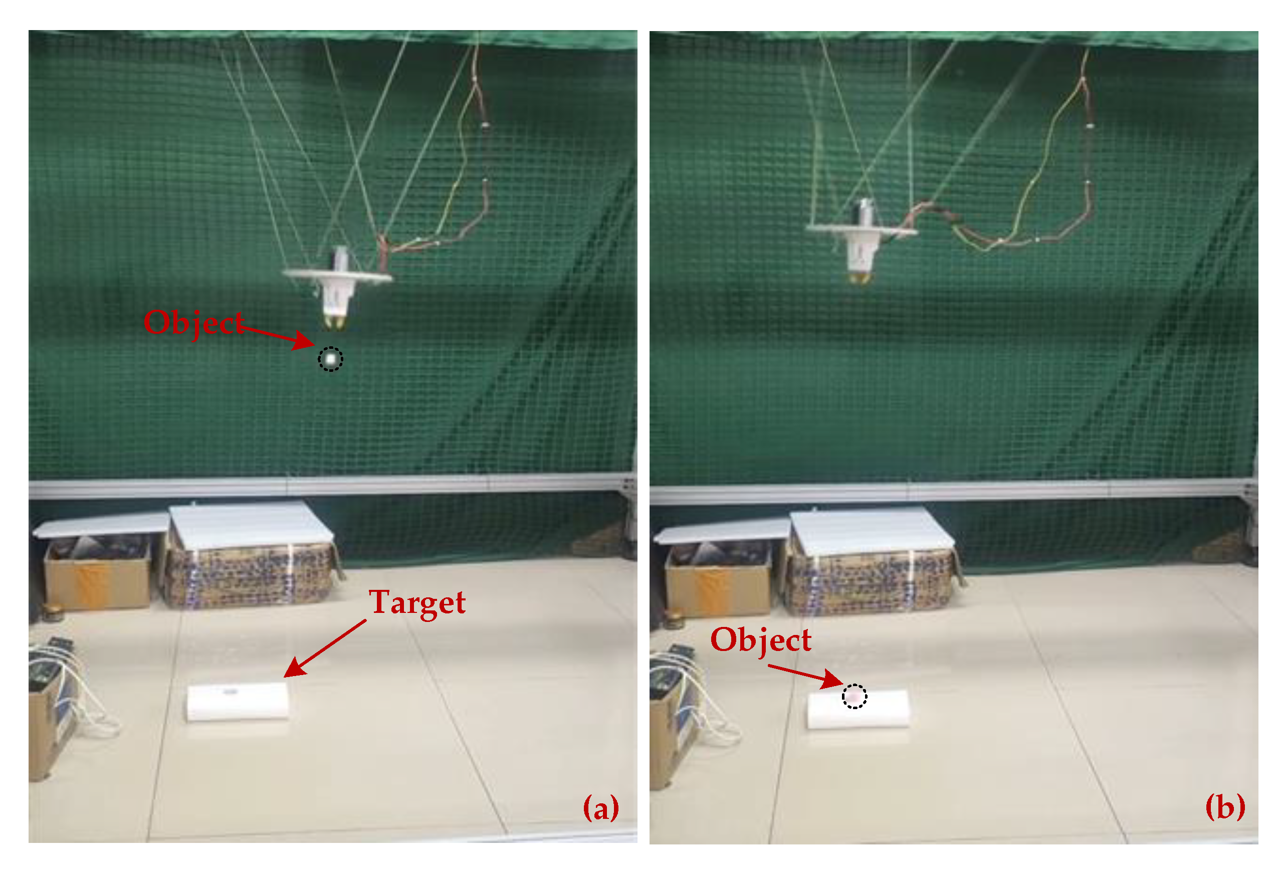
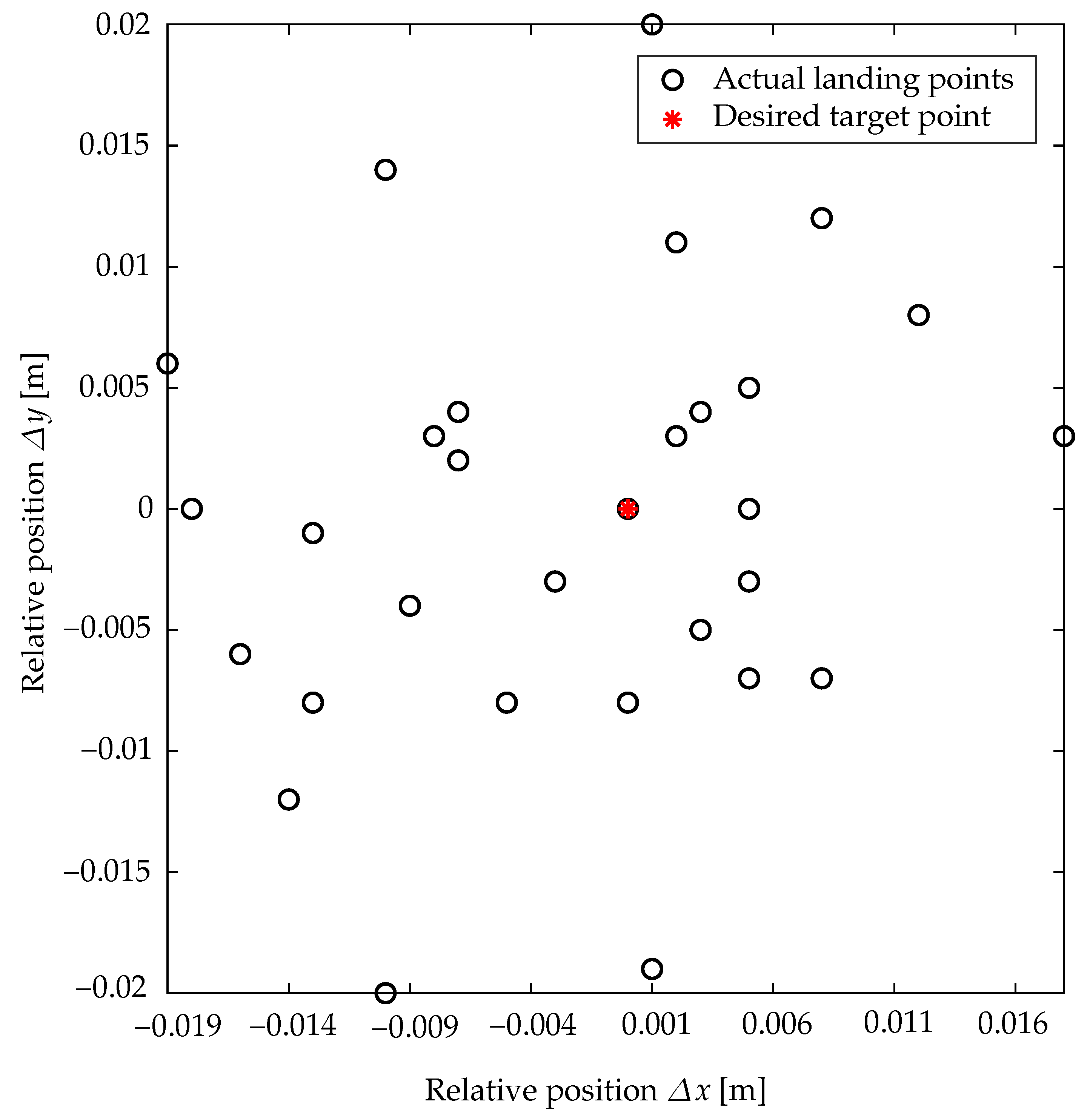
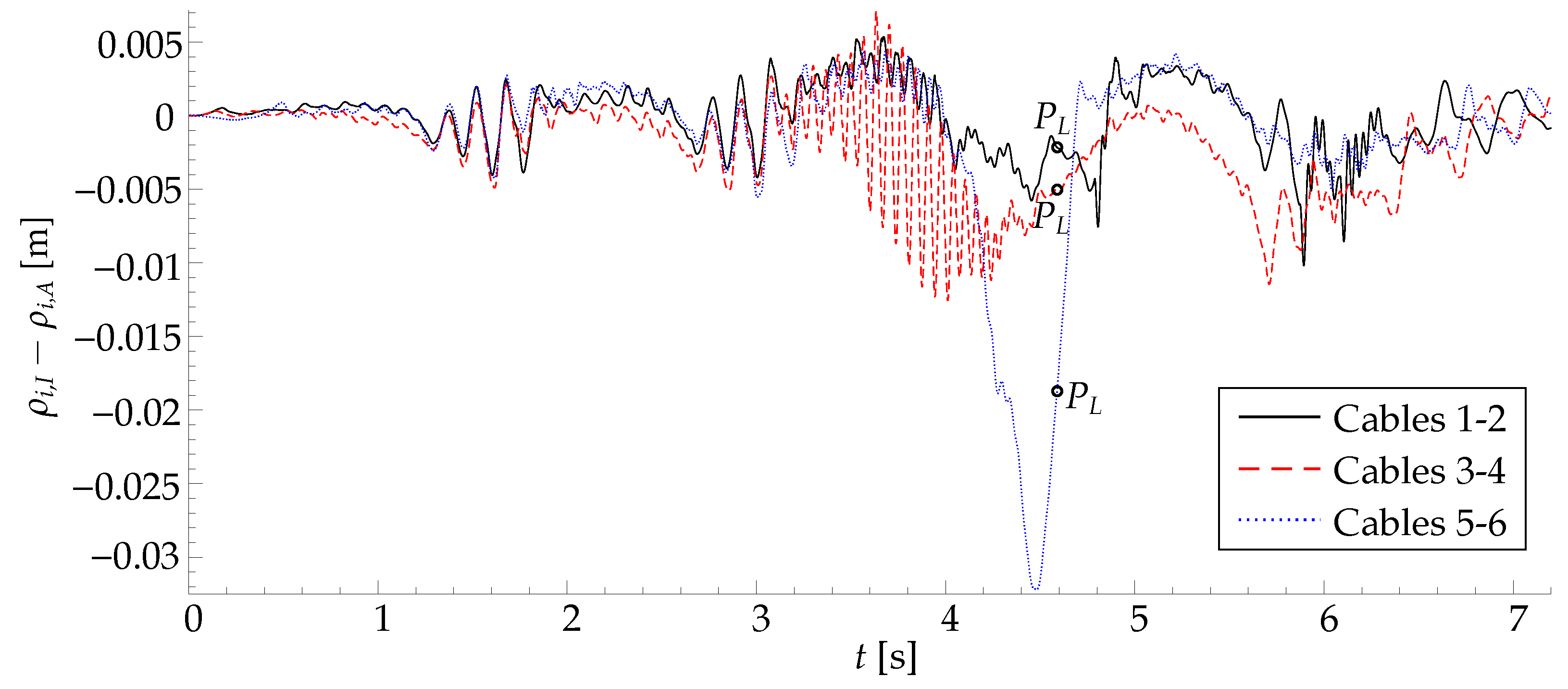
To illustrate the advantages of our approach based on Bézier curves, we also compared it with another point-to-point trajectory design method: namely, piecewise-linear trajectory segments between target points $T_i$, where the position along the segment is a fifth-order polynomial function of time [27].

These trajectories are defined as follows:

$${\mathbf{p}}_i\left(t_i^{\prime }\right)={\mathbf{t}}_i+({\mathbf{t}}_{i+1}-{\mathbf{t}}_i)u\left(\tau \right),\tau =\frac{t_i^{\prime }}{\Delta t_i}$$

(35)

where $u\left(\tau \right)$ is given by [60]

$$u\left(\tau \right)=6{\tau }^5-15{\tau }^4+10{\tau }^3$$

(36)

In Figure 7 and Figure 8, we report the plots of the cable tensions over time, as obtained by simulations, for the two trajectory planning methods; in both cases, the EE follows the example motion from Figure 6, visiting all $T_i$’s in the same sequence. Each plot shows the sum ${\tau }_{tot,ij}$ of the tensions in the pair of cables i and j; indeed, with the special architecture in Figure 3, it is sufficient [11] to verify that ${\tau }_{tot,12}$, ${\tau }_{tot,34}$ and ${\tau }_{tot,56}$ are all positive when confirming the feasibility, and the ratios between tensions ${\tau }_i/{\tau }_{tot,ij}$ always remain the same.

It can be seen from the plots that the cable tensions are always positive during the motion, which shows the feasibility of the trajectories, as expected. However, unlike the trajectory planning method in [27], with our approach, there is no need to discretize the motion to verify its feasibility.

From Equations (4) and (5), it can be seen that the cable tensions depend on the mass and the inertia of the EE. In our simulations, we consider the launch to be instantaneous and disregard the inertial properties of the launched object with respect to those of the EE, which is acceptable in most cases (for instance, in our prototype, the object being thrown has a mass of ≊20 g). Therefore, there are no discontinuities in the plots of the tensions; in any case, the sudden change in the EE mass after the object is detached does not change the sign of the tensions; therefore, the feasibility analysis provided in Section 3.2 does not change.

Figure 9 and Figure 10 show the plots of the velocity components (along the x-, y- and z-axes) of point P on the EE. As required by the motion constraints (12c), the velocity at each target point is zero for both types of trajectories; for the launch motion (Figure 9), the velocity is $\dot{\mathbf{p}}$ at the launch point $P_L$. Compared with the polynomial-based trajectory, the trajectory based on Bézier curves leads to a motion that has comparable cable tensions, even if the EE velocity has higher oscillations between $T_4$ and $T_5$ (to achieve the launch motion).

The acceleration, like the velocity, is continuous during motion, as seen in Figure 11 and Figure 12 (for the two trajectory types considered here). Notice that, with the polynomial-based trajectories from [27], the acceleration along the vertical direction must be zero at the target points, while, with Bézier curves, we do not need to add such a constraint.

5.3. Experiments

To further verify the correctness and effectiveness of the launch trajectories proposed here, experiments were carried out on an experimental prototype, which was designed according to the parameters provided in Equations (30) and (31); the final design is shown in Figure 13. A gripper has been attached to the EE, which can be opened and closed to grasp and launch objects.

Figure 14 shows an example launch motion with our prototype. The gripper opens at launch point $P_L$ and then the launched object reaches the target point, corresponding to the opening of a bin on the floor. An example launch is shown in the multimedia attachment for this work (see Video Abstract). Although some cables vibrate during the motion, this is likely due to the limitations of the prototype, and the cables still remain under tension until the launch occurs. The loss of tension could then be due to vibrations induced by the tension discontinuity caused by the sudden variation in the EE mass and by the errors in tracking the ideal (feasible) motion. In any case, the target is correctly reached by the object.

To verify the repeatability and accuracy of the launch motion, 30 launch tests were carried out consecutively with the prototype. All these tests correspond (ideally) to the same trajectory, which is again the one shown in Figure 6; however, due to the unavoidable errors in the control of the cable winches and of the gripper, the results slightly differ each time. The actual landing points were measured each time manually, by marking the point of contact of the thrown object on a paper sheet fixed on the ground.

The results are shown in Figure 15: here, each circle represents the actual landing point of the launched object after a launch, while the dot indicates the ideal target point. The coordinates $\Delta x$ and $\Delta y$ are the relative position errors with respect to the target point.

From the data in Figure 15, it can be seen that the relative position error magnitude $\sqrt{\Delta x^2+\Delta y^2}$ has an average of 0.011 m and a standard deviation of 0.006 m. These results can be considered satisfactory given the limitations of the prototype, which was built purely for demonstration purposes, and confirm the feasibility of the launching CDPR concept; a more developed design would likely achieve even better accuracy.

Finally, Figure 16 shows the plots of the tracking errors ${\rho }_{i,I}-{\rho }_{i,A}$ along an example launch motion from the previous tests. The ideal cable lengths ${\rho }_{i,I}$ are calculated from the desired trajectory using Equation (1), while the actual lengths ${\rho }_{i,A}$ are obtained from the feedback of the encoders on the winches. Here, again, only three plots are reported, since the cable lengths are pairwise equal. The tracking errors reach a maximum of $32.2$ mm during the motion: this result is comparable to those found with other demonstration prototypes [49]. In this case, however, the tracking errors reach higher values around the launch instant, due to the highly dynamical motion required for launch.

6. Discussion

In our tests, we have verified that the concept of using throwing trajectories (releasing an object from an EE suspended by cables) can indeed enlarge the workspace of CSPRs. The general concept has been proposed in our previous works [47,48], which however did not include an experimental section; additionally, those works only considered a simpler, less realistic model with a point-mass EE, while here we introduce a practically feasible design. To the best of our knowledge, no other works have considered CSPRs for throwing motions. This work, then, provides a first experimental demonstration of the concept, to verify that the main idea is indeed feasible. While our prototype has limitations, most notably in the control of the cable lengths and of the gripper mounted on the EE, it is proposed as a first design iteration (to be further refined and tested in future work), developed purely for demonstration purposes at this stage.

Furthermore, we also propose a simple trajectory planning method for our platform based on Bézier curves, which can be analytically proven to always provide trajectories which are feasible (where the cables always remain in tension); while other trajectories for dynamically-feasible motions of CSPRs have been proposed in the literature, for instance based on polynomial functions of time [27] or again on Bézier curves [57], our approach provides greater flexibility in the trajectory design while leading to comparable cable tensions and also corresponds to relatively simple conditions for feasibility.

To summarize, our concept allows us to rapidly transport objects at very large distances with a simple, cost-effective architecture. A limitation of the current work is in the assumptions on the launched mass. This can neither be too small, as air drag effects may be non-negligible, nor too large, since this may introduce large discontinuities in the cable tensions at launch. Future research may include considering more realistic (non-parabolic) ballistic trajectories for the launched mass, including drag effects, and a trajectory design that minimizes tension discontinuities.

7. Conclusions

In this work, we propose a point-to-point launch trajectory planning method based on Bézier curves and apply it on a purely translational CSPR controlled by three winches; each winch actuates two cables, which form a parallelogram. This architecture was chosen due to the simplicity of its dynamical analysis, as proved in previous works, and because it allows us to fully control the required positional DoFs for motion with only three motors; the orientation of the EE, on the other hand, had to be kept constant to control the launch.

Our trajectory planning method is both simple in its definition and allows the robot to pass by a series of target points, reaching each one at zero velocity, to perform operations such as grabbing objects with a gripper on the EE; these points may be far away from the robot footprint, as we take advantage of inertia forces to maintain the tautness of cables.

To further increase the workspace, we also propose using launch motions from the EE towards a target. We show how to define the trajectory parameters, taking into account the desired target and the trajectory feasibility, which was also verified by simulations.

Finally, we performed repeated tests on a laboratory prototype, which showed that the launch motions have sufficient repeatability and accuracy for industrial applications. To the best of our knowledge, no other tests on CSPR prototypes for launch motions have been presented in the available literature.

Our goals for future work are as follows:

• In our tests, for simplicity, we used PD control for the cable winches. This, however, was found to have limited performance in the compensation for external disturbances and lower tracking accuracy. Introducing improved control algorithms may significantly increase the repeatability of the launch motions;
• The gripper on the EE is currently connected through a wire to the control system on the frame; this wire, however, may interfere with the robot cables. A wireless control system for the gripper will increase performance;
• Improve the method used for measuring the motion of the launched object; a computer-vision-based system will be used, to avoid interference with the ballistic motion;
• Our tests indicate that discontinuities in the cable tensions will occur after the launch, which may lead to losing control of the robot, especially if the mass of the launched object is not negligible with respect to that of the EE. Optimizing the trajectory planning to minimize said discontinuities appears to be a promising option.

References

1. Lawrence, L.C. Skycam: An aerial robotic camera system. Byte 1985, 10, 122–132. [Google Scholar]
2. Lamaury, J.; Gouttefarde, M. Control of a large redundantly actuated cable-suspended parallel robot. In Proceedings of the 2013 IEEE International Conference on Robotics and Automation, Karlsruhe, Germany, 6–10 May 2013. [Google Scholar] [CrossRef]
3. Nan, R.; Li, D.; Jin, C.; Wang, Q.; Zhu, L.; Zhu, W.; Zhang, H.; Yue, Y.; Qian, L. The five-hundred-meter aperture spherical radio telescope (FAST) project. Int. J. Mod. Phys. D 2011, 20, 989–1024. [Google Scholar] [CrossRef]
4. Riechel, A.T.; Ebert-Uphoff, I. Force-feasible workspace analysis for underconstrained, point-mass cable robots. In Proceedings of the IEEE International Conference on Robotics and Automation, New Orleans, LA, USA, 26 April–1 May 2004; Volume 5, pp. 4956–4962. [Google Scholar] [CrossRef]
5. Gosselin, C.M. Global planning of dynamically feasible trajectories for three-DOF spatial cable-suspended parallel robots. In 1st International Conference on Cable-Driven Parallel Robots; Gouttefarde, M., Bruckmann, T., Pott, A., Eds.; Springer: Stuttgart, Germany, 2013; pp. 3–22. [Google Scholar] [CrossRef]
6. Jiang, X.; Barnett, E.; Gosselin, C.M. Dynamic point-to-point trajectory planning beyond the static workspace for six-DOF cable-suspended parallel robots. IEEE Trans. Robot. 2018, 34, 1–13. [Google Scholar] [CrossRef]
7. Mattioni, V.; Idà, E.; Carricato, M. Design of a planar cable-driven parallel robot for non-contact tasks. Appl. Sci. 2021, 20, 9491. [Google Scholar] [CrossRef]
8. Vu, D.S.; Barnett, E.; Zaccarin, A.; Gosselin, C.M. On the design of a three-DOF cable-suspended parallel robot based on a parallelogram arrangement of the cables. In 3rd International Conference on Cable-Driven Parallel Robots; Gosselin, C.M., Cardou, P., Bruckmann, T., Pott, A., Eds.; Springer: Québec, QC, Canada, 2018; pp. 319–330. [Google Scholar] [CrossRef]
9. Bosscher, P.; Williams, R.; Tummino, M. A concept for rapidly-deployable cable robot search and rescue systems. In Proceedings of the ASME 2005 IDETC/CIE, Long Beach, CA, USA, 24–28 September 2005; pp. 589–598. [Google Scholar] [CrossRef]
10. Barnett, E.; Gosselin, C.M. Large-scale 3D printing with a cable-suspended robot. Addit. Manuf. 2015, 7, 27–44. [Google Scholar] [CrossRef]
11. Mottola, G.; Gosselin, C.M.; Carricato, M. Dynamically feasible motions of a class of purely-translational cable-suspended parallel robots. Mech. Mach. Theory. 2019, 132, 193–206. [Google Scholar] [CrossRef]
12. Bosscher, P.; Williams, R.; Bryson, L.; Castro-Lacouture, D. Cable-suspended robotic contour crafting system. Autom. Constr. 2007, 17, 45–55. [Google Scholar] [CrossRef]
13. Castelli, G.; Ottaviano, E.; Rea, P. A Cartesian cable-suspended robot for improving end-users’ mobility in an urban environment. Robot. Comput. Integr. Manuf. 2014, 30, 335–343. [Google Scholar] [CrossRef]
14. Idà, E.; Nanetti, F.; Mottola, G. An alternative parallel mechanism for horizontal positioning of a nozzle in an FDM 3D printer. Machines 2022, 7, 542. [Google Scholar] [CrossRef]
15. Alikhani, A.; Behzadipour, S.; Alasty, A.; Vanini, S. Design of a large-scale cable-driven robot with translational motion. Robot. Comput. Integr. Manuf. 2011, 27, 357–366. [Google Scholar] [CrossRef]
16. Saber, O. A spatial translational cable robot. ASME J. Mech. Rob. 2015, 7, 031006. [Google Scholar] [CrossRef]
17. Sciarra, G.; Rasheed, T.; Mattioni, V.; Cardou, P.; Caro, S. Design and kinetostatic modeling of a cable-driven Schönflies-motion generator. In Proceedings of the ASME 2022 IDETC/CIE, St. Louis, MO, USA, 14–17 August 2022; p. V007T07A020. [Google Scholar] [CrossRef]
18. Wang, R.; Li, S.; Li, Y. A suspended cable-driven parallel robot with articulated reconfigurable moving platform for Schönflies motions. IEEE/ASME Trans. Mechatron. 2022, 27, 5173–5184. [Google Scholar] [CrossRef]
19. Behzadipour, S.; Khajepour, A. A new cable-based parallel robot with three degrees of freedom. Multibody Syst. Dyn. 2005, 13, 371–383. [Google Scholar] [CrossRef]
20. Zhang, Z.; Shao, Z.; Wang, L. Optimization and implementation of a high-speed 3-DOFs translational cable-driven parallel robot. Mech. Mach. Theory. 2020, 145, 103693. [Google Scholar] [CrossRef]
21. Barrette, G.; Gosselin, C.M. Determination of the dynamic workspace of cable-driven planar parallel mechanisms. ASME J. Mech. Des. 2005, 127, 242–248. [Google Scholar] [CrossRef]
22. Idà, E.; Briot, S.; Carricato, M. Robust trajectory planning of under-actuated cable-driven parallel robot with 3 cables. In Advances in Robot Kinematics; Lenarčič, J., Siciliano, B., Eds.; Springer International Publishing: Ljubljana, Slovenia, 2020; pp. 65–72. [Google Scholar] [CrossRef]
23. Mottola, G.; Gosselin, C.M.; Carricato, M. Dynamically feasible periodic trajectories for generic spatial three-degree-of-freedom cable-suspended parallel robots. ASME J. Mech. Rob. 2018, 10, 031004. [Google Scholar] [CrossRef]
24. Jiang, X.; Lin, D.; Li, Q. Dynamically feasible transition trajectory planning for three-dof cable-suspended parallel robots. In Proceedings of the 2019 IEEE 9th Annual International Conference on CYBER Technology in Automation, Control, and Intelligent Systems (CYBER), Suzhou, China, 29 July–2 August 2019; pp. 789–794. [Google Scholar] [CrossRef]
25. Lefrançois, S.; Gosselin, C.M. Point-to-point motion control of a pendulum-like 3-DOF underactuated cable-driven robot. In Proceedings of the 2010 IEEE International Conference on Robotics and Automation, Anchorage, AK, USA, 3–7 May 2010; pp. 5187–5193. [Google Scholar] [CrossRef]
26. Zanotto, D.; Rosati, G.; Agrawal, S.K. Modeling and control of a 3-DOF pendulum-like manipulator. In Proceedings of the 2011 IEEE International Conference on Robotics and Automation, Shanghai, China, 9–13 May 2011; pp. 3964–3969. [Google Scholar] [CrossRef]
27. Gosselin, C.M.; Foucault, S. Dynamic point-to-point trajectory planning of a two-DOF cable-suspended parallel robot. IEEE Trans. Robot. 2014, 30, 728–736. [Google Scholar] [CrossRef]
28. Jiang, X.; Gosselin, C.M. Dynamic point-to-point trajectory planning of a three-DOF cable-suspended parallel robot. IEEE Trans. Robot. 2016, 32, 1550–1557. [Google Scholar] [CrossRef]
29. Zhang, N.; Shang, W.; Cong, S. Geometry-based trajectory planning of a 3-3 cable-suspended parallel robot. IEEE Trans. Robot. 2016, 33, 484–491. [Google Scholar] [CrossRef]
30. Dion-Gauvin, P.; Gosselin, C.M. Dynamic point-to-point trajectory planning of a three-DOF cable-suspended mechanism using the hypocycloid curve. IEEE/ASME Trans. Mechatron. 2018, 23, 1964–1972. [Google Scholar] [CrossRef]
31. Mottola, G.; Gosselin, C.M.; Carricato, M. Dynamically-feasible elliptical trajectories for fully constrained 3-DOF cable-suspended parallel robots. In 3rd International Conference on Cable-Driven Parallel Robots; Gosselin, C.M., Cardou, P., Bruckmann, T., Pott, A., Eds.; Springer: Québec, QC, Canada, 2018; pp. 219–230. [Google Scholar] [CrossRef]
32. Zhang, N.; Shang, W. Dynamic trajectory planning of a 3-DOF under-constrained cable-driven parallel robot. Mech. Mach. Theory. 2016, 98, 21–35. [Google Scholar] [CrossRef]
33. Dion-Gauvin, P.; Gosselin, C.M. Beyond-the-static-workspace point-to-point trajectory planning of a 6-DoF cable-suspended mechanism using oscillating SLERP. Mech. Mach. Theory. 2022, 174, 104894. [Google Scholar] [CrossRef]
34. Raptopoulos, F.; Koskinopoulou, M.; Maniadakis, M. Robotic pick-and-toss facilitates urban waste sorting. In Proceedings of the 2020 IEEE 16th International Conference on Automation Science and Engineering (CASE), Hong Kong, China, 20–21 August 2020; pp. 1149–1154. [Google Scholar] [CrossRef]
35. Reist, P.; D’Andrea, R. Design and analysis of a blind juggling robot. IEEE Trans. Robot. 2012, 28, 1228–1243. [Google Scholar] [CrossRef]
36. Fagiolini, A.; Torelli, A.; Bicchi, A. Casting robotic end-effectors to reach far objects in space and planetary missions. In Proceedings of the 9th ESA Workshop on Advanced Space Technologies for Robotics and Automation, Noordwijk, The Netherlands, November 28–30 2006. [Google Scholar]
37. Arisumi, H.; Otsuki, M.; Nishida, S. Launching penetrator by casting manipulator system. In Proceedings of the 2012 IEEE/RSJ International Conference on Intelligent Robots and Systems, Vilamoura-Algarve, Portugal, 7–12 October 2012; pp. 5052–5058. [Google Scholar] [CrossRef]
38. Hatakeyama, T.; Mochiyama, H. Shooting manipulation inspired by chameleon. IEEE/ASME Trans. Mechatron. 2013, 18, 527–535. [Google Scholar] [CrossRef]
39. Asgari, M.; Nikoobin, A. A variational approach to determination of maximum throw-able workspace of robotic manipulators in optimal ball pitching motion. Trans. Inst. Meas. Control 2021, 43, 2378–2391. [Google Scholar] [CrossRef]
40. Zeng, A.; Song, S.; Lee, J.; Rodriguez, A.; Funkhouser, T. TossingBot: Learning to throw arbitrary objects with residual physics. IEEE Trans. Robot. 2020, 36, 1307–1319. [Google Scholar] [CrossRef]
41. Hassan, G.; Chemori, A.; Gouttefarde, M.; El Rafei, M.; Francis, C.; Hervé, P.E.; Sallé, D. A novel extended desired compensation adaptive law for high-speed pick-and-throw with PKMs. In Proceedings of the 14th IFAC International Workshop on Adaptation and Learning in Control and Signal Processing, Casablanca, Morocco, 29 June–1 July 2022; pp. 627–633. [Google Scholar] [CrossRef]
42. Hassan, G.; Gouttefarde, M.; Chemori, A.; Hervé, P.E.; El Rafei, M.; Francis, C.; Sallé, D. Time-optimal pick-and-throw S-curve trajectories for fast parallel robots. IEEE/ASME Trans. Mechatron. 2022, 27, 4707–4717. [Google Scholar] [CrossRef]
43. Frank, H.; Wellerdick-Wojtasik, N.; Hagebeuker, B.; Novak, G.; Mahlknecht, S. Throwing objects—A bio-inspired approach for the transportation of parts. In Proceedings of the 2006 IEEE International Conference on Robotics and Biomimetics, Kunming, China, 17–20 December 2006; pp. 91–96. [Google Scholar] [CrossRef]
44. Frank, T.; Janoske, U.; Mittnacht, A.; Schroedter, C. Automated throwing and capturing of cylinder-shaped objects. In Proceedings of the IEEE 2012 ICRA, Saint Paul, MN, USA, 14–18 May 2012; pp. 5264–5270. [Google Scholar] [CrossRef]
45. Fischer, O.; Toshimitsu, Y.; Kazemipour, A.; Katzschmann, R.K. Dynamic control of soft manipulators to perform real-world tasks. arXiv 2022, arXiv:2201.02151. [Google Scholar] [CrossRef]
46. Ruggiero, F.; Lippiello, V.; Siciliano, B. Nonprehensile dynamic manipulation: A survey. IEEE Robot. Autom. Lett. 2018, 3, 1711–1718. [Google Scholar] [CrossRef]
47. Lin, D.; Mottola, G.; Carricato, M.; Jiang, X. Modeling and control of a cable-suspended sling-like parallel robot for throwing operations. Appl. Sci. 2020, 10, 9067. [Google Scholar] [CrossRef]
48. Lin, D.; Mottola, G.; Carricato, M.; Jiang, X.; Li, Q. Dynamically-feasible trajectories for a cable-suspended robot performing throwing operations. In Proceedings of the ROMANSY 23 Symposium on Robot Design, Dynamics and Control; Springer: Berlin/Heidelberg, Germany, 2020; pp. 547–555. [Google Scholar] [CrossRef]
49. Mottola, G.; Gosselin, C.M.; Carricato, M. Effect of actuation errors on a purely-translational spatial cable-driven parallel robot. In Proceedings of the 2019 IEEE 9th Annual International Conference on CYBER Technology in Automation, Control, and Intelligent Systems (CYBER), Suzhou, China, 29 July–2 August 2019; pp. 701–707. [Google Scholar] [CrossRef]
50. Salisbury, J. Active stiffness control of a manipulator in Cartesian coordinates. In Proceedings of the 1980 IEEE Conference on Decision and Control, Albuquerque, NM, USA, 10–12 December 1980; pp. 95–100. [Google Scholar] [CrossRef]
51. Yoshikawa, T. Analysis and control of robot manipulators with redundancy. In Proceedings of the 1st International Symposium on Robotics Research, Bretton Woods, NH, USA, 25 August–2 September 1983. [Google Scholar]
52. Cardou, P.; Bouchard, S.; Gosselin, C.M. Kinematic-sensitivity indices for dimensionally nonhomogeneous Jacobian matrices. IEEE Trans. Robot. 2010, 26, 166–173. [Google Scholar] [CrossRef]
53. Merlet, J.P. Jacobian, manipulability, condition number, and accuracy of parallel robots. ASME J. Mech. Rob. 2006, 128, 199–206. [Google Scholar] [CrossRef]
54. Patel, S.; Sobh, T. Manipulator performance measures-a comprehensive literature survey. J. Intell. Robot. Syst. 2015, 77, 547–570. [Google Scholar] [CrossRef]
55. Bernstein, D.S. Matrix Mathematics: Theory, Facts, and Formulas; Princeton University Press: Princeton, NJ, USA, 2009. [Google Scholar] [CrossRef]
56. Piegl, L.; Tiller, W. The NURBS Book; Monographs in Visual Communication; Springer: Berlin/Heidelberg, Germany, 1996. [Google Scholar] [CrossRef]
57. Zhang, N.; Shang, W.; Cong, S. Dynamic trajectory planning for a spatial 3-DoF cable-suspended parallel robot. Mech. Mach. Theory. 2018, 122, 177–196. [Google Scholar] [CrossRef]
58. Qian, S.; Bao, K.; Zi, B.; Zhu, W.D. Dynamic trajectory planning for a three degrees-of-freedom cable-driven parallel robot using quintic B-splines. ASME J. Mech. Des. 2020, 142, 073301. [Google Scholar] [CrossRef]
59. Tempel, P.; Schnelle, F.; Pott, A.; Eberhard, P. Design and programming for cable-driven parallel robots in the German Pavilion at the EXPO 2015. Machines 2015, 3, 223–241. [Google Scholar] [CrossRef]
60. Biagiotti, L.; Melchiorri, C. Trajectory Planning for Automatic Machines and Robots; Springer Science & Business Media: Berlin/Heidelberg, Germany, 2008. [Google Scholar] [CrossRef]
Figure 1. A launch motion: the EE starts at C, moves along a trajectory and launches an object at P L .
Machines 11 00224 g001
Figure 2. Schematic of a point-to-point motion where the CSPR has to pass through a number of target points T i , which may also be outside the SEW, and launch an object towards a target point P T .
Machines 11 00224 g002
Figure 3. Schematic of a spatial, six-cable CSPR with parallelogram actuation; P is the CoM of the EE.
Machines 11 00224 g003
Figure 4. The parallelogram defined by cables 5 and 6; the fixed and mobile frames are also shown.
Machines 11 00224 g004
Figure 5. Top view of the CDPR under exam at a reference position.
Machines 11 00224 g005
Figure 6. Example point-to-point launch trajectory defined by a series of consecutive Bézier curves.
Machines 11 00224 g006
Figure 7. Plot of the cable tensions during motion for the trajectory defined by Bézier curves.
Machines 11 00224 g007
Figure 8. As Figure 7, for the trajectory defined by fifth-order polynomial segments.
Machines 11 00224 g008
Figure 9. Plot of the velocity components of P, for the Bézier curve trajectory.
Machines 11 00224 g009
Figure 10. As Figure 9, for the trajectory defined by fifth-order polynomial segments.
Machines 11 00224 g010
Figure 11. Plot of the acceleration components of P, for the Bézier curve trajectory.
Machines 11 00224 g011
Figure 12. As Figure 11, for the trajectory defined by fifth-order polynomial segments.
Machines 11 00224 g012
Figure 13. The six-cable CSPR prototype used for the launch motion tests.
Machines 11 00224 g013
Figure 14. An example launch: the gripper mounted on the EE opens and the carried object is released (frame (a)). The object then moves towards the target along a parabolic trajectory (b).
Machines 11 00224 g014
Figure 15. The actual landing points measured in 30 successive tests.
Machines 11 00224 g015
Figure 16. Cable length errors between the ideal cable lengths ρ i , I and the actual ones ρ i , A during a launch along the trajectory in Figure 6. The launch occurs at P L .
Machines 11 00224 g016
Disclaimer/Publisher’s Note: The statements, opinions and data contained in all publications are solely those of the individual author(s) and contributor(s) and not of MDPI and/or the editor(s). MDPI and/or the editor(s) disclaim responsibility for any injury to people or property resulting from any ideas, methods, instructions or products referred to in the content.