Dynamics Modeling and Redundant Force Optimization of Modular Combination Parallel Manipulator

Abstract

The limb-driving force mutation of the modular combination parallel manipulator (MCPM) affects the alignment process of optical axis. In this paper, a novel optimization method based on the force mutation penalty term is proposed to solve the problem of driving force mutation. The kinematics and dynamics models of the manipulator are established using a modularization idea, reducing the complexity of the modeling process, and verified using co-simulation. Moreover, particle swarm optimization (PSO) is applied as an optimization tool. The effectiveness of the proposed method is confirmed by comparing it with the minimize-the-maximum and Moore–Penrose (M–P) methods, which are widely used to solve parallel manipulators with redundant drives.

1. Introduction

The alignment of the optical axis of a small aperture space optical remote sensor in space environment simulator is achieved with the Stewart parallel manipulator. With the increase in the aperture, the requirements for the size of the moving platform and load capacity of the Stewart parallel manipulator increase. The traditional six-point support structure will lead to large deformation of the moving platform, severe stress concentration at the support point, excessive driving force, and other problems. The load capacity of the parallel manipulator can be increased without increasing the height and driving force by splicing the platforms together.

Many scholars have researched kinematics and dynamics on the parallel manipulator [1,2,3,4]. Most of the research on the MCPM focuses on the combination of the drive unit as a module or the parallel manipulator as a module. Arrouk et al. [5] designed a 3-CRS parallel kinematic machine (PRM) consisting of three modular kinematic chains. Tang et al. [6] designed a new modular-based hybrid PRM using the joint as a module. Zhang et al. [7] designed a generalized spherical parallel mechanism with partially decoupled characteristics by combining position and orientation modules. Hao et al. [8] used identical spatial modules to construct a large-range modular XYZ compliant parallel manipulator. Until now, the research of parallel manipulators with redundant actuation focuses on adding one or several redundant drives based on a particular configuration. Wu et al. [9] added an RRR leg to the planar 2-RRR parallel mechanism. Xi et al. [10] added a redundant leg to the three-degrees-of-freedom (DOF) tricept parallel mechanism. Yao et al. [11] added actuation to the middle PRPU branch of the 5UPS parallel platform. Zhao et al. [12] added two PSS legs to the planar 6PSS parallel manipulator. However, there are few studies on the Stewart platform as a modular, redundant unit.

The dynamics equation of parallel manipulator with redundant actuation is non-homogeneous linear equations [13], with multiple solutions to the driving force. Xu et al. [14] used the Moore–Penrose (M–P) method to solve the driving force of redundant parallel manipulators and discussed whether the calculation results contain internal forces. Xie et al. [15] developed a novel 3DOF parallel mechanism driven by four legs and solved the driving force distribution using the least squares norm method. Lee et al. [16] studied the actuator power consumption of a 3-RRR fully planar parallel manipulator and proposed a driving force optimization method to minimize the electrical energy consumed, finding that 26% of energy could be saved. Jiang et al. [17] designed a novel planar 2-DOF parallel kinematic machine with kinematic redundancy, and a method for redundant force optimization is presented to improve the precision of the machine. Hino et al. [18] used minimize-the-maximum actuator force as the objective function, using the linear matrix inequality method to solve the actuator force. Wu et al. [19] used the minimum actuator torque range into account and proposed a novel torque optimization method of a 3-DOF redundantly actuated parallel manipulator for friction stir welding. The primary methods of redundant force distribution are the M-P method [20,21,22], minimum norm method [23,24,25,26], minimum energy consumption method [27,28,29], minimum structural deformation method [30,31], maximize manipulator accuracy [32,33], and minimize-the-maximum driving force method [9,34]. The driving force mutation of the modular combination parallel manipulator (MCPM) will affect the alignment process of the optical axis. However, these methods solve the driving force independently at each discrete point of the trajectory; the change in the driving force of the adjacent discrete points is not considered.

In this paper, we proposed a novel optimization method based on the force mutation penalty term to solve force mutation of the MCPM. Moreover, particle swarm optimization (PSO) is applied as optimization tool. The proposed method is compared with the minimize-the-maximum and M-P methods (i.e., least squares method) moving along the same trajectory. The remainder of this paper is organized as follows. In the next section, the structure and inverse kinematics of the MCPM is analyzed. Then, its dynamic model is constructed in Section 3. In Section 4, the general solution of the driving force is deduced. Then, force mutation is minimized by optimizing the distribution of redundant force. Section 5 gives two simulation examples of MCPM to verify the proposed method’s effectiveness. Finally, the conclusions of this paper are provided.

2. Structure Description and Inverse Kinematics

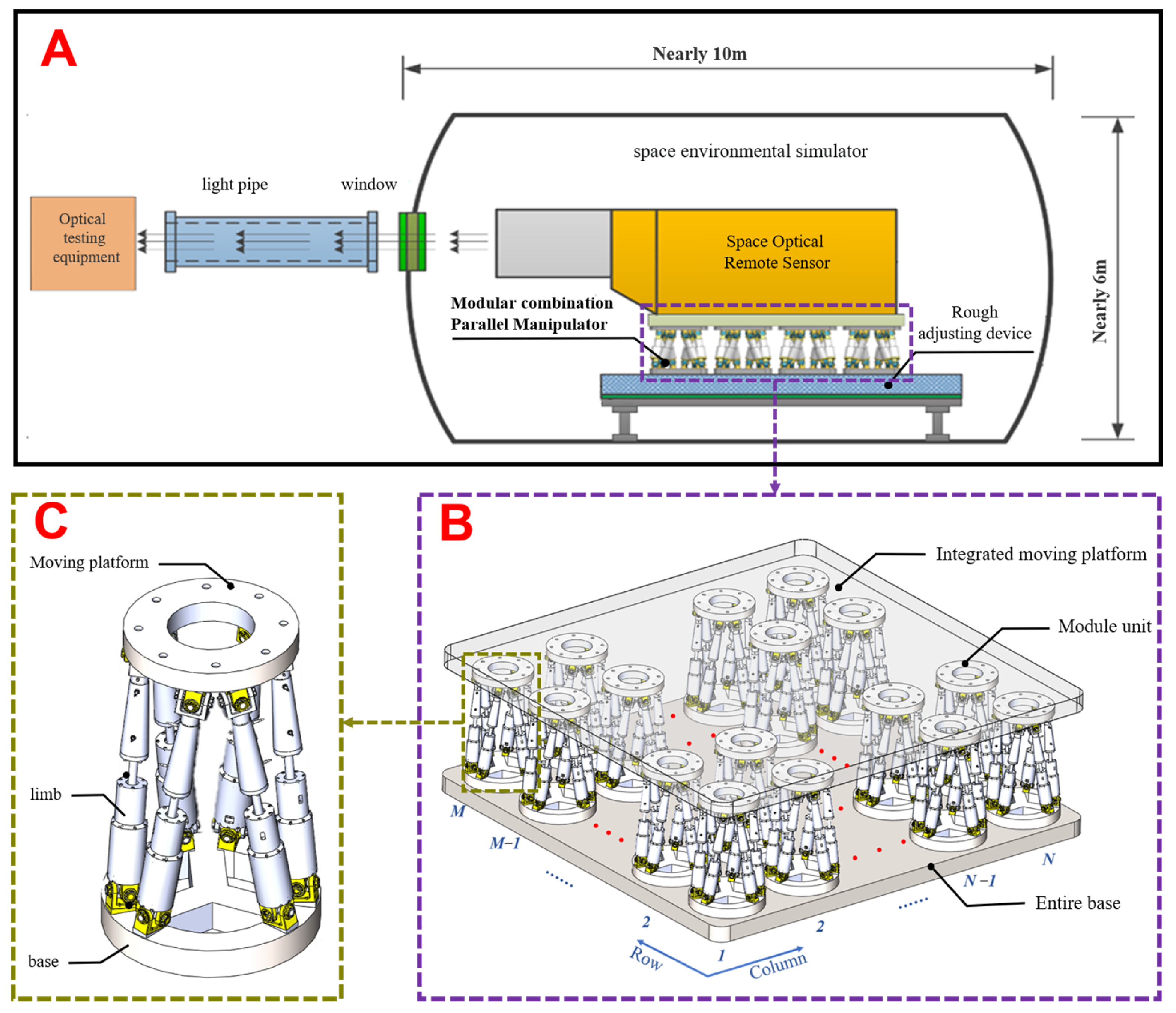
2.1. Structure Description

A modular combination parallel manipulator (MCPM) is developed for the optical axis alignment of a space optical remote sensor with an aperture over two meters in a space environment simulator. As depicted in Figure 1, the modular combination parallel manipulator (MCPM) comprises M × N 6-DOF parallel platforms, each module unit consisting of a moving platform, base, and 6-UPU limbs. Each base is connected to the entire base, and each moving platform is connected to the integrated moving platform. The space optical remote sensor is installed above the integrated moving platform. A rough adjustment device and MCPM are used to achieve rough and accurate optical axis alignment in the space environment simulator. First, the space optical remote sensor opens the imaging function and makes the target in the light pipe within the imaging range by adjusting the rough adjusting device. Then, make the target in the middle of the image by adjusting the MCPM.

2.2. Inverse Kinematics

This section uses a modularization idea to establish the MCPM kinematic model. The modeling process of the modularization idea is as follows. Firstly, the global systems are established on the MCPM level, and the coordinate systems for internal use are established at the module unit level. Then, the kinematic analysis between MCPM and module unit is carried out at the MCPM level. Finally, the kinematics analysis is carried out on the module unit level.

As illustrated in Figure 2A, an integrated moving coordinate system $\left\{\mathit{P}\right\}\left\{P-X_P{Y}_P{Z}_P\right\}$ and an entire base coordinate system $\left\{\mathit{O}\right\}\left\{O-XYZ\right\}$ are established in the MCPM. The coordinate frame $\left\{\mathit{P}\right\}$ is located at the center point P of the integrated moving platform. The coordinate frame $\left\{\mathit{O}\right\}$ is attached to the entire base at its center point O. As depicted in Figure 2B, a module moving coordinate system $\left\{{\mathit{P}}_{ij}\right\}\left\{P_{ij}-{}^{X}p_{ij}{Y}_{p_{ij}}{Z}_{p_{ij}}\right\}$, module base coordinate system $\left\{{\mathit{O}}_{ij}\right\}\left\{O_{ij}-X_{O_{ij}}{Y}_{O_{ij}}{Z}_{O_{ij}}\right\}$, and six limbs coordinate system are established in the module unit ij, which is located in row i and column j. The coordinate frame $\left\{{\mathit{P}}_{ij}\right\}$ is located at the center point $P_{ij}$ of the moving platform. The coordinate frame $\left\{{\mathit{O}}_{ij}\right\}$ is attached to the base at its center point $O_{ij}$. Six limb coordinate systems $\left\{{\mathit{A}}_{ij}^{\left(k\right)}\right\}\left\{a_{ij}^{\left(k\right)}-X_{a_{ij}^{\left(k\right)}}{Y}_{a_{ij}^{\left(k\right)}}{Z}_{a_{ij}^{\left(k\right)}}\right\}$ are fixed to each limb and located at the center of the joint $a_{ij}^{\left(k\right)}$ connecting the base and the limb. The $Z_{a_{ij}^{\left(k\right)}}$ axis points from $a_{ij}^{\left(k\right)}$ to $b_{ij}^{\left(k\right)}$; the $Y_{a_{ij}^{\left(k\right)}}$ axis is parallel to the cross product of two unit vectors of the $Z_{O_{ij}}$ and $Z_{a_{ij}^{\left(k\right)}}$ axes; the $X_{a_{ij}^{\left(k\right)}}$ axis is defined by the right hand. The frame $\left\{\mathit{O}\right\}$ and $\left\{{\mathit{O}}_{ij}\right\}$ are in parallel. The frame $\left\{\mathit{P}\right\}$ and $\left\{{\mathit{P}}_{ij}\right\}$ are also in parallel.

2.2.1. Kinematic Analysis between MCPM and Module Unit

Velocity transformation between the integrated moving platform and moving platform of the module unit ij in frame $\left\{\mathit{O}\right\}$ can be written as

$${\mathit{v}}_{P_{ij}}={\mathit{T}}_{P_{ij}}\stackrel{·}{{\mathit{x}}_P}$$

(1)

where ${\mathit{T}}_{P_{ij}}=\left[{\mathit{E}}_{3\times 3}-\widetilde{\mathit{P}{\mathit{P}}_{ij}}\right]$ is a transformation matrix.

According to the transformation formula between different coordinate systems, moving platform’s velocity ${\mathit{v}}_{P_{ij}}$ can be transferred to the frame $\left\{{\mathit{O}}_{ij}\right\}$ as follows:

$${}^{{\mathit{O}}_{ij}}\mathit{v}_{P_{ij}}={}_{\mathit{O}}{}^{{\mathit{O}}_{ij}}\mathit{R}\mathit{v}_{p_{ij}}$$

(2)

where ${}_{\mathit{O}}{}^{{\mathit{O}}_{ij}}\mathit{R}$ is the rotation matrix of frame $\left\{\mathit{O}\right\}$ relative to frame $\left\{{\mathit{O}}_{ij}\right\}$.

Substituting Equation (1) into Equation (2) yields

$${}^{{\mathit{O}}_{ij}}\mathit{v}_{P_{ij}}={}_P{}^{P_{ij}}\mathit{J}\stackrel{·}{{\mathit{x}}_P}$$

(3)

where ${}_P{}^{P_{ij}}\mathit{J}={}_{\mathit{O}}{}^{{\mathit{O}}_{ij}}\mathit{R}{\mathit{T}}_{P_{ij}}$.

2.2.2. Module Unit Inverse Kinematics

As depicted in Figure 2B, the closed-loop vector equation for each limb of module unit ij can be written as

$${}^{{\mathit{O}}_{ij}}{\mathit{d}}_{ij}^{\left(k\right)}+{}^{{\mathit{O}}_{ij}}{\mathit{o}}_{ij}{\mathit{a}}_{ij}^{\left(k\right)}={}^{{\mathit{O}}_{ij}}{\mathit{o}}_{ij}{\mathit{p}}_{ij}+{}_{{\mathit{P}}_{ij}}{}^{{\mathit{O}}_{ij}}\mathit{R}^{{\mathit{P}}_{ij}}{\mathit{p}}_{ij}{\mathit{b}}_{ij}^{\left(k\right)}$$

(4)

where ${}_{{\mathit{P}}_{ij}}{}^{{\mathit{O}}_{ij}}\mathit{R}$ is the rotation matrix of frame $\left\{{\mathit{P}}_{ij}\right\}$ relative to frame $\left\{{\mathit{O}}_{ij}\right\}$.

The velocity of joint $b_{ij}^{\left(k\right)}$ is found by the time derivative of Equation (4).

$${}^{{\mathit{O}}_{ij}}\mathit{v}_{b_{ij}^{\left(k\right)}}={}_{P_{ij}}{}^{b_{ij}^{\left(k\right)}}\mathit{T}\stackrel{·}{{}^{{\mathit{O}}_{ij}}\mathit{x}_{P_{ij}}}$$

(5)

where ${}_{P_{ij}}{}^{b_{ij}^{\left(k\right)}}\mathit{T}=\left[{\mathit{E}}_{3\times 3}-\stackrel{~}{{}^{{\mathit{O}}_{ij}}{\mathit{P}}_{ij}{\mathit{b}}_{ij}^{\left(k\right)}}\right]$ is a transformation matrix.

The velocity of joint $b_{ij}^{\left(k\right)}$ can be transferred to frame $\left\{{\mathit{A}}_{ij}^{\left(k\right)}\right\}$.

$${}^{{\mathit{A}}_{ij}^{\left(k\right)}}\mathit{v}_{b_{ij}^{\left(k\right)}}={}_{{\mathit{O}}_{ij}}{}^{{\mathit{A}}_{ij}^{\left(k\right)}}\mathit{R}{}^{{\mathit{O}}_{ij}}\mathit{v}_{b_{ij}^{\left(k\right)}}$$

(6)

where ${}_{{\mathit{O}}_{ij}}{}^{{\mathit{A}}_{ij}^{\left(k\right)}}\mathit{R}$ is the rotation matrix of frame $\left\{{\mathit{O}}_{ij}\right\}$ relative to frame $\left\{{\mathit{A}}_{ij}^{\left(k\right)}\right\}$.

Substituting Equation (5) into (6) yields

$${}^{{\mathit{A}}_{ij}^{\left(k\right)}}\mathit{v}_{b_{ij}^{\left(k\right)}}={}_{P_{ij}}{}^{b_{ij}^{\left(k\right)}}\mathit{J}\stackrel{·}{{}^{{\mathit{O}}_{ij}}\mathit{x}_{P_{ij}}}$$

(7)

where ${}_{P_{ij}}{}^{b_{ij}^{\left(k\right)}}\mathit{J}={}_{{\mathit{O}}_{ij}}{}^{{\mathit{A}}_{ij}^{\left(k\right)}}\mathit{R}{}_{P_{ij}}{}^{b_{ij}^{\left(k\right)}}\mathit{T}$.

In frame $\left\{{\mathit{A}}_{ij}^{\left(k\right)}\right\}$, the angular velocity of the kth limb can be written as

$${}^{{\mathit{A}}_{ij}^{\left(k\right)}}\mathit{\omega }=\frac{1}{d_{a_{ij}^{\left(k\right)}}}\left({}^{{\mathit{A}}_{ij}^{\left(k\right)}}\mathit{s}\times {}^{{\mathit{A}}_{ij}^{\left(k\right)}}\mathit{v}_{b_{ij}^{\left(k\right)}}\right)$$

(8)

where $d_{a_{ij}^{\left(k\right)}}$ is the distance between joints $a_{ij}^{\left(k\right)}$ and $b_{ij}^{\left(k\right)}$, and ${}^{{\mathit{A}}_{ij}^{\left(k\right)}}\mathit{s}=\left[\begin{array}{ccc}0& 0& 1\end{array}\right]$ is the unit vector of the kth limb in frame $\left\{{\mathit{A}}_{ij}^{\left(k\right)}\right\}$.

Substituting Equation (7) into (8) yields

$${}^{{\mathit{A}}_{ij}^{\left(k\right)}}\mathit{\omega }={}_{P_{ij}}{}^{a_{ij}^{\left(k\right)}}{\mathit{J}}_{\omega }\stackrel{·}{{}^{{\mathit{O}}_{ij}}\mathit{x}_{P_{ij}}}$$

(9)

where ${}_{P_{ij}}{}^{{}_{a_{ij}^{\left(k\right)}}}\mathit{J}_{\omega }=\frac{1}{d_{a_{ij}^{\left(k\right)}}}{}^{{\mathit{A}}_{ij}^{\stackrel{\sim }{\left(k\right)}}}\mathit{S}^{b_{ij}^{\left(k\right)}}{}_{P_{ij}}\mathit{J}$.

In the kth limb, the velocity of the cylinder’s centroid and piston’s centroid can be expressed as

$${}^{{\mathit{A}}_{ij}^{\left(k\right)}}\mathit{v}_{a_{ij}^{\left(k1\right)}}=l_1{}^{{\mathit{A}}_{ij}^{\left(k\right)}}\mathit{\omega }\times {}^{{\mathit{A}}_{ij}^{\left(k\right)}}\mathit{s}$$

(10)

$${}^{{\mathit{A}}_{ij}^{\left(k\right)}}\mathit{v}_{a_{ij}^{\left(k2\right)}}=\left(d_{a_{ij}^{\left(k\right)}}-l_2\right){}^{{\mathit{A}}_{ij}^{\left(k\right)}}\mathit{\omega }\times {}^{{\mathit{A}}_{ij}^{\left(k\right)}}\mathit{s}+\stackrel{·}{d_{a_{ij}^{\left(k\right)}}}{}^{{\mathit{A}}_{ij}^{\left(k\right)}}\mathit{s}$$

(11)

where $l_1$ is the distance between joint $a_{ij}^{\left(k\right)}$ and the kth cylinder’s centroid, and $l_2$ is between joint $b_{ij}^{\left(k\right)}$ and the kth piston’s centroid.

Substituting Equations (7) and (8) into Equations (10) and (11) yields

$${}^{{\mathit{A}}_{ij}^{\left(k\right)}}\mathit{v}_{a_{ij}^{\left(k1\right)}}={}_{P_{ij}}{}^{a_{ij}^{\left(k1\right)}}\mathit{J}\stackrel{·}{{}^{{\mathit{O}}_{ij}}\mathit{x}_{P_{ij}}}$$

(12)

$${}^{{\mathit{A}}_{ij}^{\left(k\right)}}\mathit{v}_{a_{ij}^{\left(k2\right)}}={}_{P_{ij}}{}^{a_{ij}^{\left(k2\right)}}\mathit{J}\stackrel{·}{{}^{{\mathit{O}}_{ij}}\mathit{x}_{P_{ij}}}$$

(13)

where

${}_{P_{ij}}{}^{a_{ij}^{\left(k1\right)}}\mathit{J}=-\frac{l_1}{d_{a_{ij}^{\left(k\right)}}}\stackrel{\sim }{{}^{{\mathit{A}}_{ij}^{\left(k\right)}}\mathit{S}}\stackrel{\sim }{{}^{{\mathit{A}}_{ij}^{\left(k\right)}}\mathit{S}}{}_{P_{ij}}{}^{b_{ij}^{\left(k\right)}}\mathit{J}$,

${}_{P_{ij}}{}^{a_{ij}^{\left(k2\right)}}\mathit{J}=\left[{}^{{\mathit{A}}_{ij}^{\left(k\right)}}\mathit{s}-\frac{d_{a_{ij}^{\left(k\right)}}-l_2}{d_{a_{ij}^{\left(k\right)}}}\stackrel{\sim }{{}^{{\mathit{A}}_{ij}^{\left(k\right)}}\mathit{S}}\stackrel{\sim }{{}^{{\mathit{A}}_{ij}^{\left(k\right)}}\mathit{S}}\right]{}_{P_{ij}}{}^{b_{ij}^{\left(k\right)}}\mathit{J}$.

3. Inverse Dynamics

In this section, a modularization idea is used to establish the MCPM dynamical model. The modeling process of the modularization idea is as follows. Firstly, analyze the applied and inertia force of MCPM. Then, analyze the applied and inertia force of the module unit. Finally, the dynamic model of the entire system is derived using the virtual work principle.

3.1. MCPM Applied and Inertia Force

Assume that the mass of load is $m_z$, the mass of integrated moving platform is $m_p$, and the integrated moving platform is subjected to the external force ${\mathit{F}}_{ij}$ acting on point $O_{ij}$ by module unit ij. The applied and inertia forces imposed on the load’s centroid $P_z$ and integrated moving platform’s centroid $P$ can be expressed as Equations (14) and (15).

$${\mathit{F}}_z=\left[\begin{array}{c}{m}_z\mathit{g}-m_z\stackrel{·}{{\mathit{v}}_z}\\ -{\mathit{I}}_z\stackrel{·}{{\mathit{\omega }}_p}-{\mathit{\omega }}_p\times \left({\mathit{I}}_z{\mathit{\omega }}_p\right)\end{array}\right]$$

(14)

$${\mathit{F}}_p=\left[\begin{array}{c}{m}_p\mathit{g}-m_p\stackrel{·}{{\mathit{v}}_p}\\ -{\mathit{I}}_p\stackrel{·}{{\mathit{\omega }}_p}-{\mathit{\omega }}_p\times \left({\mathit{I}}_p{\mathit{\omega }}_p\right)\end{array}\right]$$

(15)

3.2. Module Unit Applied and Inertia Force

Assuming that module unit ij is subjected to the external force $-{\mathit{F}}_{ij}$ acting on point $O_{ij}$ by the integrated moving platform. In frame $\left\{{\mathit{O}}_{ij}\right\}$, the applied and inertia force ${}^{{\mathit{O}}_{ij}}\mathit{F}_{P_{ij}}$ imposed on the center of moving platform can be expressed as Equation (16). In frame $\left\{{\mathit{A}}_{ij}^{\left(k\right)}\right\}$, the applied and inertia forces imposed on the kth cylinder’s centroid and piston’s centroid can be expressed as Equations (17) and (18).

$${}^{{\mathit{O}}_{ij}}\mathit{F}_{P_{ij}}=\left[\begin{array}{c}{m}_{p_{ij}}{}_{\mathit{O}}{}^{{\mathit{O}}_{ij}}\mathit{R}\mathit{g}-m_{p_{ij}}\stackrel{·}{{}^{{\mathit{O}}_{ij}}\mathit{v}_{P_{ij}}}\\ -{}^{{\mathit{O}}_{ij}}\mathit{I}_{P_{ij}}\stackrel{·}{{}^{{\mathit{O}}_{ij}}\mathit{\omega }_{P_{ij}}}-{}^{{\mathit{O}}_{ij}}\mathit{\omega }_{P_{ij}}\times \left({}^{{\mathit{O}}_{ij}}\mathit{I}_{P_{ij}}{}^{{\mathit{O}}_{ij}}\mathit{\omega }_{P_{ij}}\right)\end{array}\right]$$

(16)

$${}^{{\mathit{A}}_{ij}^{\left(k\right)}}\mathit{F}_{a_{ij}^{\left(k1\right)}}=\left[\begin{array}{c}{m}_{a_{ij}^{\left(k1\right)}}{}_{{\mathit{O}}_{ij}}{}^{{\mathit{A}}_{ij}^{\left(k\right)}}\mathit{R}\mathit{g}-m_{a_{ij}^{\left(k1\right)}}\stackrel{·}{{}^{{\mathit{A}}_{ij}^{\left(k\right)}}\mathit{v}_{a_{ij}^{\left(k1\right)}}}\\ -{}^{{\mathit{A}}_{ij}^{\left(k\right)}}\mathit{I}_{a_{ij}^{\left(k1\right)}}\stackrel{·}{{}^{{\mathit{A}}_{ij}^{\left(k\right)}}\mathit{\omega }}-{}^{{\mathit{A}}_{ij}^{\left(k\right)}}\mathit{\omega }\times \left({}^{{\mathit{A}}_{ij}^{\left(k\right)}}\mathit{I}_{a_{ij}^{\left(k1\right)}}{}^{{\mathit{A}}_{ij}^{\left(k\right)}}\mathit{\omega }\right)\end{array}\right]$$

(17)

$${}^{{\mathit{A}}_{ij}^{\left(k\right)}}\mathit{F}_{a_{ij}^{\left(k2\right)}}=\left[\begin{array}{c}{m}_{a_{ij}^{\left(k2\right)}}{}_{{\mathit{O}}_{ij}}{}^{{\mathit{A}}_{ij}^{\left(k\right)}}\mathit{R}\mathit{g}-m_{a_{ij}^{\left(k2\right)}}\stackrel{·}{{}^{{\mathit{A}}_{ij}^{\left(k\right)}}\mathit{v}_{a_{ij}^{\left(k2\right)}}}\\ -{}^{{\mathit{A}}_{ij}^{\left(k\right)}}\mathit{I}_{a_{ij}^{\left(k2\right)}}\stackrel{·}{{}^{{\mathit{A}}_{ij}^{\left(k\right)}}\mathit{\omega }}-{}^{{\mathit{A}}_{ij}^{\left(k\right)}}\mathit{\omega }\times \left({}^{{\mathit{A}}_{ij}^{\left(k\right)}}\mathit{I}_{a_{ij}^{\left(k2\right)}}{}^{{\mathit{A}}_{ij}^{\left(k\right)}}\mathit{\omega }\right)\end{array}\right]$$

(18)

3.3. Dynamics Equation

The dynamics equation of the entire system is established based on the principle of virtual work.

$$\begin{array}{l}{\left(\delta ,{\mathit{x}}_z\right)}^{\mathrm{T}}{\mathit{F}}_{\mathrm{z}}+{\left(\delta {\mathit{x}}_p\right)}^{\mathrm{T}}{\mathit{F}}_p+{\displaystyle \sum _{j=1}^N{\displaystyle \sum _{i=1}^M{\left(\delta {\mathit{x}}_{P_{ij}}\right)}^{\mathrm{T}}{\mathit{F}}_{ij}}}+\cdots \\ {\displaystyle \sum _{j=1}^N{\displaystyle \sum _{i=1}^M\left[{\displaystyle \sum _{k=1}^6\left({\left({}^{{\mathit{A}}_{ij}^{\left(k\right)}}\delta \mathit{x}_{b_{ij}^{\left(k\right)}}\right)}^{\mathrm{T}}{}^{{\mathit{A}}_{ij}^{\left(k\right)}}\mathit{\tau }+{\left({}^{{\mathit{A}}_{ij}^{\left(k\right)}}\delta \mathit{x}_{a_{ij}^{\left(k1\right)}}\right)}^{\mathrm{T}}{}^{{\mathit{A}}_{ij}^{\left(k\right)}}\mathit{F}_{a_{ij}^{\left(k1\right)}}+\right.}\right.}}\cdots \\ \left.\left.{\left({}^{{\mathit{A}}_{ij}^{\left(k\right)}}\delta {\mathit{x}}_{a_{ij}^{\left(k2\right)}}\right)}^{\mathrm{T}}{}^{{\mathit{A}}_{ij}^{\left(k\right)}}\mathit{F}_{a_{ij}^{\left(k2\right)}}\right)+{\left({}^{{\mathit{O}}_{ij}}\delta {\mathit{x}}_{P_{ij}}\right)}^{\mathrm{T}}{}^{{\mathit{O}}_{ij}}\mathit{F}_{P_{ij}}+{\left(\delta {\mathit{x}}_p\right)}^{\mathrm{T}}\left(-{\mathit{F}}_{ij}\right)\right]=0,\end{array}$$

(19)

where ${}^{\mathit{H}}\delta {\mathit{x}}_e$ means a virtual displacement of point e in frame $\left\{\mathit{H}\right\}$, and ${}^{{\mathit{A}}_{ij}^{\left(k\right)}}\mathit{\tau }$ is the driving force of the kth limb in frame $\left\{{\mathit{A}}_{ij}^{\left(k\right)}\right\}$.

Based on the previous kinematics analysis, the virtual displacement can be expressed as follows

$$\left\{\begin{array}{l}{}^{{\mathit{O}}_{ij}}\delta {\mathit{x}}_{P_{ij}}={\mathit{T}}_{ij}\delta {\mathit{x}}_p\\ {}^{{\mathit{A}}_{ij}^{\left(k\right)}}\delta {\mathit{x}}_{b_{ij}^{\left(k\right)}}={\mathit{T}}_{ij}^{\left(k\right)}{}^{{\mathit{O}}_{ij}}\delta {\mathit{x}}_{P_{ij}}\\ {}^{{\mathit{A}}_{ij}^{\left(k\right)}}\delta {\mathit{x}}_{a_{ij}^{\left(k1\right)}}={\mathit{T}}_{ij}^{\left(k1\right)}{}^{{\mathit{O}}_{ij}}\delta {\mathit{x}}_{P_{ij}}\\ {}^{{\mathit{A}}_{ij}^{\left(k\right)}}\delta {\mathit{x}}_{a_{ij}^{\left(k2\right)}}={\mathit{T}}_{ij}^{\left(k2\right)}{}^{{\mathit{O}}_{ij}}\delta {\mathit{x}}_{P_{ij}}\end{array}\right.$$

(20)

where ${\mathit{T}}_{ij}$, ${\mathit{T}}_{ij}^{\left(k\right)}$, ${\mathit{T}}_{ij}^{\left(k1\right)}$ and ${\mathit{T}}_{ij}^{\left(k2\right)}$ are virtual displacement transformation matrices.

Assuming that the load is fixed on the integrated moving platform, it’s virtual displacement equation can be easily obtained using the inverse kinematics.

$$\delta {\mathit{x}}_z={\mathit{T}}_L\delta {\mathit{x}}_p$$

(21)

where ${\mathit{T}}_L$ is the transformation matrix of $\delta {\mathit{x}}_p$ relative to $\delta {\mathit{x}}_z$.

Substituting Equations (20) and (21) into Equation (19) yields

$$\begin{array}{l}{\left(\delta {\mathit{x}}_p\right)}^{\mathrm{T}}\left\{{\left({\mathit{T}}_L\right)}^{\mathrm{T}}{\mathit{F}}_{\mathrm{z}}+{\mathit{F}}_p+\cdots \right.\\ {\displaystyle \sum _{j=1}^N{\displaystyle \sum _{i=1}^M{\left({\mathit{T}}_{ij}\right)}^{\mathrm{T}}\left[{\displaystyle \sum _{k=1}^6\left({\left({\mathit{T}}_{ij}^{\left(k\right)}\right)}^{\mathrm{T}}{}^{{\mathit{A}}_{ij}^{\left(k\right)}}\mathit{\tau }+{\left({\mathit{T}}_{ij}^{\left(k1\right)}\right)}^{\mathrm{T}}{}^{{\mathit{A}}_{ij}^{\left(k\right)}}\mathit{F}_{a_{ij}^{\left(k1\right)}}+\left.{\left({\mathit{T}}_{ij}^{\left(k2\right)}\right)}^{\mathrm{T}}{}^{{\mathit{A}}_{ij}^{\left(k\right)}}\mathit{F}_{a_{ij}^{\left(k2\right)}}\right)\right.}\right.}}\\ \left.\left.\cdots +{}^{{\mathit{O}}_{ij}}\mathit{F}_{P_{ij}}\right]\right\}=0\end{array}$$

(22)

Because Equation (22) applies to any $\delta x_p$, it can be rewritten as

$$\begin{array}{l}{\left({\mathit{T}}_L\right)}^{\mathrm{T}}{\mathit{F}}_{\mathrm{z}}+{\mathit{F}}_p+\cdots \\ {\displaystyle \sum _{j=1}^N{\displaystyle \sum _{i=1}^M{\left({\mathit{T}}_{ij}\right)}^{\mathrm{T}}\left[{\displaystyle \sum _{k=1}^6\left({\left({\mathit{T}}_{ij}^{\left(k\right)}\right)}^{\mathrm{T}}{}^{{\mathit{A}}_{ij}^{\left(k\right)}}\mathit{\tau }+{\left({\mathit{T}}_{ij}^{\left(k1\right)}\right)}^{\mathrm{T}}{}^{{\mathit{A}}_{ij}^{\left(k\right)}}\mathit{F}_{a_{ij}^{\left(k1\right)}}+\left.{\left({\mathit{T}}_{ij}^{\left(k2\right)}\right)}^{\mathrm{T}}{}^{{\mathit{A}}_{ij}^{\left(k\right)}}\mathit{F}_{a_{ij}^{\left(k2\right)}}\right)\right.}\right.}}\\ \left.\cdots +{}^{{\mathit{O}}_{ij}}\mathit{F}_{P_{ij}}\right]=0\end{array}$$

(23)

After variable substitution, Equation (23) can be simplified as

$${\mathit{J}}_{\mathrm{z}}{\mathit{F}}_z+{\mathit{F}}_{\mathit{H}}+\mathit{J}\mathit{\tau }+{\mathit{J}}_1{\mathit{F}}_1+{\mathit{J}}_2{\mathit{F}}_2=0,$$

(24)

where ${\mathit{J}}_{\mathrm{z}}={\left({\mathit{T}}_L\right)}^{\mathrm{T}}$,

${\mathit{F}}_{\mathit{H}}={\mathit{F}}_p+{\displaystyle \sum _{j=1}^N{\displaystyle \sum _{i=1}^M{\left({\mathit{T}}_{ij}\right)}^{\mathrm{T}}{}^{{\mathit{O}}_{ij}}\mathit{F}_{P_{ij}}}}$,

$\mathit{J}={\left[{\mathit{J}}_{11}^{\left(1\right)}\cdots {\mathit{J}}_{11}^{\left(6\right)}{\mathit{J}}_{21}^{\left(1\right)}\cdots {\mathit{J}}_{ij}^{\left(k\right)}\cdots {\mathit{J}}_{MN}^{\left(6\right)}\right]}^{\mathrm{T}}$ where ${\mathit{J}}_{ij}^{\left(k\right)}={\left({\mathit{T}}_{ij}\right)}^{\mathrm{T}}{\left({\mathit{T}}_{ij}^{\left(k\right)}\right)}^{\mathrm{T}}$,

$\mathit{\tau }=\left[{}^{{\mathit{A}}_{11}^{\left(1\right)}}\mathit{\tau }\cdots {}^{{\mathit{A}}_{11}^{\left(6\right)}}\mathit{\tau }{}^{{\mathit{A}}_{21}^{\left(1\right)}}\mathit{\tau }\cdots {}^{{\mathit{A}}_{ij}^{\left(k\right)}}\mathit{\tau }\cdots {}^{{\mathit{A}}_{MN}^{\left(6\right)}}\mathit{\tau }\right]$,

${\mathit{F}}_1=\left[{}^{{\mathit{A}}_{11}^{\left(1\right)}}\mathit{F}_{a_{11}^{\left(11\right)}}\cdots {}^{{\mathit{A}}_{11}^{\left(6\right)}}\mathit{F}_{a_{11}^{\left(61\right)}}{}^{{\mathit{A}}_{12}^{\left(1\right)}}\mathit{F}_{a_{12}^{\left(11\right)}}\cdots {}^{{\mathit{A}}_{ij}^{\left(k\right)}}\mathit{F}_{a_{ij}^{\left(k1\right)}}\cdots {}^{{\mathit{A}}_{MN}^{\left(6\right)}}\mathit{F}_{a_{MN}^{\left(61\right)}}\right]$,

${\mathit{J}}_1={\left[{\mathit{J}}_{11}^{\left(1\right)}\cdots {\mathit{J}}_{11}^{\left(6\right)}{\mathit{J}}_{21}^{\left(1\right)}\cdots {\mathit{J}}_{ij}^{\left(k\right)}\cdots {\mathit{J}}_{MN}^{\left(6\right)}\right]}^{\mathrm{T}}$ where ${\mathit{J}}_{ij}^{\left(k\right)}={\left({\mathit{T}}_{ij}\right)}^{\mathrm{T}}{\left({\mathit{T}}_{ij}^{\left(k1\right)}\right)}^{\mathrm{T}}$,

${\mathit{F}}_2=\left[{}^{{\mathit{A}}_{11}^{\left(1\right)}}\mathit{F}_{a_{11}^{\left(12\right)}}\cdots {}^{{\mathit{A}}_{11}^{\left(6\right)}}\mathit{F}_{a_{11}^{\left(62\right)}}{}^{{\mathit{A}}_{12}^{\left(1\right)}}\mathit{F}_{a_{12}^{\left(12\right)}}\cdots {}^{{\mathit{A}}_{ij}^{\left(k\right)}}\mathit{F}_{a_{ij}^{\left(k2\right)}}\cdots {}^{{\mathit{A}}_{MN}^{\left(6\right)}}\mathit{F}_{a_{MN}^{\left(62\right)}}\right]$,

${\mathit{J}}_2={\left[{\mathit{J}}_{11}^{\left(1\right)}\cdots {\mathit{J}}_{11}^{\left(6\right)}{\mathit{J}}_{21}^{\left(1\right)}\cdots {\mathit{J}}_{ij}^{\left(k\right)}\cdots {\mathit{J}}_{MN}^{\left(6\right)}\right]}^{\mathrm{T}}$ where ${\mathit{J}}_{ij}^{\left(k\right)}={\left({\mathit{T}}_{ij}\right)}^{\mathrm{T}}{\left({\mathit{T}}_{ij}^{\left(k2\right)}\right)}^{\mathrm{T}}$.

where ${\mathit{J}}_{\mathrm{z}}$, $\mathit{J}$, ${\mathit{J}}_1$, and ${\mathit{J}}_2$ are transformation matrices, which could convert ${\mathit{F}}_z$, $\mathit{\tau }$, ${\mathit{F}}_1$, and ${\mathit{F}}_2$ to frame $\left\{\mathit{O}\right\}$ and translate point of force action to point P at the same time, ${\mathit{F}}_1$ and ${\mathit{F}}_2$ are vectors of resultant of applied and inertia wrenches exerted at cylinder’s and piston’s centroid of all limbs. $\mathit{\tau }$ is a vector of the driving force of all limbs. ${\mathit{F}}_H$ is a vector of the resultant of applied and inertia wrenches exerted at the integrated moving platform’s centroid and moving platform’s centroid of all module units.

4. Redundant Driving Force Optimization

4.1. General Solution of Driving Force

For a given load and trajectory, the dynamics equation of the MCPM is anon-homogeneous linear equation. There are multiple solutions to the limb-driving force. For Equation (24), based on the solution method of the non-homogeneous linear equations, the solution of limb-driving forces can be written as

$$F=C_{1}X+C_2,$$

(25)

where $C_2$ is the M-P solution which is given in Appendix A, $C_1=\mathrm{N}(\mathit{J})$ is the null space matrix of $\mathit{J}$, $X=\left[\begin{array}{ccc}{x}_1& \cdots x_i\cdots & x_{6\times \left(M\times N-1\right)}\end{array}\right]$ is $1\times \left(6\times \left(M\times N-1\right)\right)$ constant matrix, and $x_i\in \left(-\infty ,+\infty \right)$. By taking different $x_i$ values, we can obtain an infinite number of solutions.

4.2. Driving Force Optimization Method

The driving force mutation of MCPM affects optical axis alignment. However, the traditional optimization method does not consider the change in the driving force of the adjacent discrete points, causing force mutation during MCPM movement. Consequently, given that the driving force in actual work is a bounded variable, too large a driving force causes the driver element to fail—a smaller driving force is more optimal. Therefore, this paper designs an improved minimize-the-maximum driving force optimization method. The improved optimization method’s objective function is to minimize the maximum value of all driving forces, with the change in the driving force multiplied by the penalty coefficient added as the penalty term. The objective optimization function of the improved optimization method can be expressed as

$$f(x)=\underset{x}{\min }\left[\underset{t}{\max }\left(\left|F_t\right|+w\times \left|F_t-F_{t-1}\right|\right)\right],$$

(26)

where $w$ is the penalty coefficient and $w\ge 0$, $w\times \left|F_t-F_{t-1}\right|$ is the penalty term, $\left|F_t\right|$ is the absolute value of F at time t in a given trajectory, $\left|F_t-F_{t-1}\right|$ is the absolute value of F change between time t and $t-1$ in the given trajectory.

The optimization results can be changed by adjusting the penalty coefficient. When the penalty coefficient $w=0$, it equals the minimize-the-maximum optimization. The optimization result is minimal driving force but with significant force mutation. When the penalty coefficient is infinitely great, it equals the minimum-force-mutation optimization. The optimization result is the minimum-force mutation but a sizeable driving force. Therefore, the reduction in force mutation is at the cost of increasing the driving force.

Minimize-the-maximum optimization is a special optimization problem. It uses the maximum value of each group to form a new group and selects the minimum value from the new group. Most previous studies on the minimize-the-maximum optimization problem are conducted under the condition of one redundant driving force. Moreover, the problem can be solved by geometric methods. However, the geometric method is no longer suitable when there are too many redundant driving forces. Therefore, this paper proposes applying PSO as the optimization tool under the condition of multiple redundant driving forces. PSO can quickly converge to the global optimal solution. For a given load and trajectory, the optimization process is depicted in Figure 3.

In the process of optical axis adjustment, the appropriate penalty coefficient value must be selected to reduce the torque of the driving element under the premise of meeting the requirements of the force mutation index. For a given load and trajectory, the procedure for determining the value of penalty coefficient can be described as follows:

Step 1. Calculate the maximum force mutation value K that the MCPM can tolerate.

Step 2. Set the initial value of $w=0$ and the search step length $\Delta w=1$.

Step 3. For the given $w$, use the method shown in Figure 3 to optimize the driving force. After optimization, the maximum driving force H and maximum force mutation U are obtained.

Step 4. If U > K, set $w=w+\Delta w$ and go to step 3; else, output the $w$ value and H value and end the program.

An appropriate penalty coefficient can be obtained after calculation by this algorithm. At this time, the maximum driving force value is minimized while the force mutation requirement is met.

5. Case Study

In order to verify the effectiveness of the dynamic model and improved optimization method presented in this research, two examples of MCPM (M = 1, N = 2 and M = 2, N = 2) are given in this section.

5.1. Inverse Kinematics and Dynamics Simulation

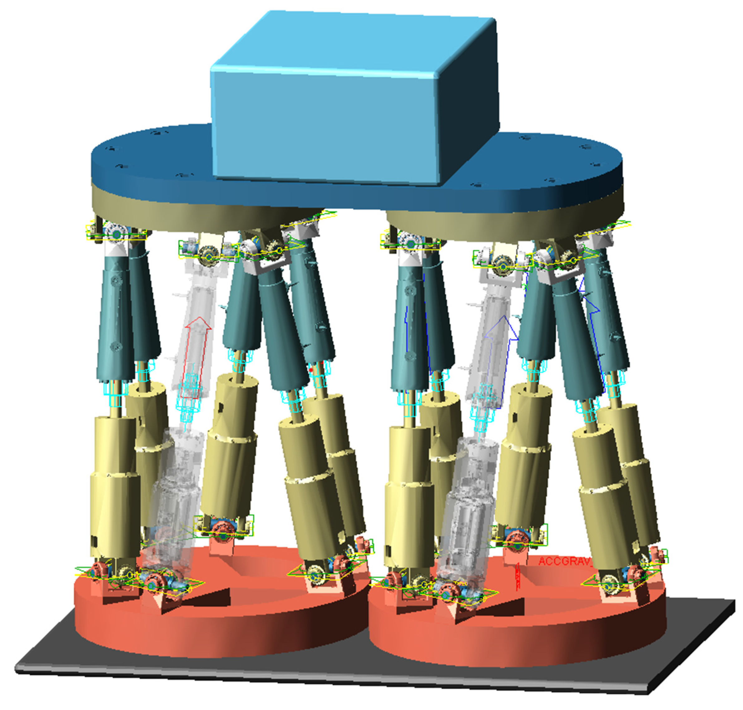
This section uses an example of MCPM (M = 1, N = 2) to prove the correctness of the dynamics modeling. Firstly, using ADAMS software to establish the dynamics model. Then, the distribution results of limb driving force in ADAMS software are obtained through the co-simulation of MATLAB and ADAMS. Finally, the simulation results obtained by two different software are the same, which verifies the correctness of the dynamic modeling.

5.1.1. ADAMS Model

ADAMS software is used to build a dynamics model of the MCPM (M = 1, N = 2). The dynamics model is depicted in Figure 4. The geometrical and inertia parameters of the module unit are presented in

Table 1. Module unit parameters.

Parameters	Value	Parameters	Value
${}^{{\mathit{O}}_{ij}}a{}_{ij}^{\left(1\right)}$	(−0.1488, −0.1416, 0.1) m	${}^{{\mathit{O}}_{ij}}b{}_{ij}^{\left(1\right)}$	(−0.1530, 0.04837, 0.6651) m
${}^{{\mathit{O}}_{ij}}a{}_{ij}^{\left(2\right)}$	(−0.04818, −0.1997, 0.1) m	${}^{{\mathit{O}}_{ij}}b{}_{ij}^{\left(2\right)}$	(0.3463, −0.1567, 0.6651) m
${}^{{\mathit{O}}_{ij}}a{}_{ij}^{\left(3\right)}$	(0.1970, −0.05810, 0.1) m	${}^{{\mathit{O}}_{ij}}b{}_{ij}^{\left(3\right)}$	(0.1184, −0.1084, 0.6651) m
${}^{{\mathit{O}}_{ij}}a{}_{ij}^{\left(4\right)}$	(0.1961, 0.05810, 0.1) m	${}^{{\mathit{O}}_{ij}}b{}_{ij}^{\left(4\right)}$	(0.1184, 0.1084, 0.6651) m
${}^{{\mathit{O}}_{ij}}a{}_{ij}^{\left(5\right)}$	(−0.04818, 0.1997, 0.1) m	${}^{{\mathit{O}}_{ij}}b{}_{ij}^{\left(5\right)}$	(0.03463, 0.1567, 0.6651) m
${}^{{\mathit{O}}_{ij}}a{}_{ij}^{\left(6\right)}$	(−0.1488, 0.1416, 0.1) m	${}^{{\mathit{O}}_{ij}}b{}_{ij}^{\left(6\right)}$	(−0.1530, 0.04837, 0.6651) m
${}^{{\mathit{O}}_{ij}}p{}_{ij}$	(0, 0, 0.7288) m	$m_{p_{ij}}$	30.68 kg
$l_1$	0.1495 m	$m_{a_{ij}^{\left(k1\right)}}$	3.089 kg
$l_2$	0.1221 m	$m_{a_{ij}^{\left(k2\right)}}$	1.825 kg
${}^{{\mathit{O}}_{ij}}\mathit{I}{}_{P_{ij}}$	$\left[\begin{array}{ccc}0.404& 0& 0\\ 0& 0.404& 0\\ 0& 0& 0.779\end{array}\right]$ kg·m2	${}^{{\mathit{A}}_{ij}^{\left(k\right)}}\mathit{I}{}_{a_{ij}^{\left(k1\right)}}$	$\left[\begin{array}{ccc} 0.0413& 0& 0\\ 0& 0.0414& 0\\ 0& 0& 0.002\end{array}\right]$ kg·m2
${}^{{\mathit{A}}_{ij}^{\left(k\right)}}\mathit{I}{}_{a_{ij}^{\left(k2\right)}}$	$\left[\begin{array}{ccc}0.0147& 0& 0\\ 0& 0.0150& 0\\ 0& 0& 0.001\end{array}\right]$ kg·m2

. The geometrical and inertia parameters of the MCPM are presented in

Table 2. MCPM parameters.

Parameters	Value	Parameters	Value
$m_z$	1000 kg	$m_p$	103.5 kg
$P_z$	(0, 0, 0.9776) m	$P$	(0, 0, 0.7776) m
$\mathit{g}$	(0, 0, −10) N/kg	${\mathit{I}}_{\mathrm{P}}$	$\left[\begin{array}{ccc}1.26& 0& 0\\ 0& 6.08& 0\\ 0& 0& 7.31\end{array}\right]$ kg·m2
$\left|p_{\left(i-1\right)j}{p}_{ij}\right|$	0.51 m	$\left|p_{i\left(j-1\right)}{p}_{ij}\right|$	0.51 m
${\mathit{I}}_z$	$\left[\begin{array}{ccc} 43.4& 0& 0\\ 0& 36.5& 0\\ 0& 0& 58.3\end{array}\right]$ kg·m2

.

5.1.2. Co-Simulation

MATLAB and ADAMS software are used for co-simulation. the simulation flow chart is depicted in Figure 5. In ADAMS, the limb of module unit 11 is driven by force, and the limb of module unit 12 is driven by motion. The penalty coefficient w is set to 500, and the given trajectory of the integrated moving platform is defined by Equation (27), where $x_p$, $y_p$, and $z_p$ are the translational motion in frame $\left\{\mathit{O}\right\}$ with time, ${\phi }_{x_p}$, ${\phi }_{y_p}$, ${\phi }_{z_p}$ are the Tait–Bryan angles extrinsic rotations motion in frame $\left\{\mathit{O}\right\}$ with time. The rotation is defined as follows: a rotation of ${\phi }_{x_p}$ about the fixed $X$ axis followed by a rotation of ${\phi }_{y_p}$ about the fixed $Y$ axis and a rotation of ${\phi }_{z_p}$ about the fixed $Z$ axis. The given position and attitude are illustrated in Figure 6A,C. The position and attitude results of the ADAMS simulation output are illustrated in Figure 6B,D. Based on Figure 6, the given trajectory and ADAMS outputs trajectory are almost identical. This finding confirms that the inverse kinematics is correct. The MATLAB and ADAMS simulation results of the limb-driving force of the module unit 12 are depicted in Figure 7. Based on Figure 7, the output driving force of each limb is identical from different software, verifying correct inverse dynamics.

$$\left\{\begin{array}{ll}{x}_p=0.010\times \sin (0.1\times t)& (\mathrm{m})\\ y_p=0.007\times \sin (0.1\times t)& (\mathrm{m})\\ z_p=0.003\times \sin (0.1\times t)+0.778& (\mathrm{m})\\ {\phi }_{x_p}=0.10\times \sin (0.1\times t)& (\mathrm{rad})\\ {\phi }_{y_p}=0.07\times \sin (0.1\times t)& (\mathrm{rad})\\ {\phi }_{z_p}=0.03\times \sin (0.1\times t)& (\mathrm{rad})\end{array}\right.\begin{array}{cc}& \begin{array}{l}t\in \left(0,20\pi \right)\\ \Delta t=0.1(\mathrm{s})\end{array}\end{array}$$

(27)

5.2. Redundant-Force-Optimization Method Simulation

This section uses the M-P, minimize-the-maximum, and improved optimization methods to calculate the driving force of MCPM (M = 1, N = 2 and M = 2, N = 2) in the given trajectory to confirm the superiority of the improved optimization method. The penalty coefficients of the improved optimization method are set as 0, 30, 50, 100, 200, 300, 500, and 800 for calculation. When w = 0, the improved optimization method is equal to the minimize-the-maximum method.

The driving force calculation results of the three types of optimization methods are depicted in Figure 8 and Figure 9 (each optimization result curve takes the maximum of the absolute value of all driving forces at a discrete point-in-time of the trajectory as source data). Based on Figure 8 and Figure 9, for each discrete point of the trajectory, the maximum driving force increases as the penalty coefficient increases, although they are larger than the minimize-the-maximum method but much smaller than the M-P method.

The force mutations of the three types of optimization methods are depicted in Figure 10 (each force mutation curve takes the maximum of the absolute value of all force mutation at a discrete point-in-time of the trajectory as source data). As depicted in Figure 10A and Figure 11A, for each discrete point of the trajectory, the force mutation value decreases with the increase in the penalty coefficient. Moreover, they are all much smaller than the minimize-the-maximum method. As depicted in Figure 10B and Figure 11B, the force mutation is better than the M-P method when the penalty coefficient is greater than a specific value.

The maximum driving forces and force mutations of the three types of optimization methods are depicted in Figure 12 and Figure 13 (each column takes the maximum of the absolute value of the driving force or force mutation of the entire trajectory as source data). Based on Figure 12 and Figure 13, for the entire trajectory, compared with the minimize-the-maximum driving force method, the maximum force value increases slightly after introducing the penalty term, but the force mutation decreases significantly. Moreover, by choosing appropriate penalty coefficients (w = 300, 500, and 800), the maximum driving force and force mutation are both smaller than the M-P method. In particular, the maximum driving force decreased significantly.

6. Conclusions

This paper investigates the driving force of the limb optimization method of the MCPM by taking force mutation into account. A novel optimization method based on the force mutation penalty term is proposed to solve the problem of force mutation. The PSO has been considered the optimization tool under multiple redundant driving forces. The performance of the proposed method is simulated with a series of w values. Compared with the minimize-the-maximum driving force method, the maximum force value increases slightly after introducing the penalty term, but the force mutation decreases significantly. Compared with the widely used M-P method, the proposed method can reduce both the maximum driving force and force mutation. Especially, the maximum driving force decreased significantly. The simulation results verify the effectiveness of the proposed optimization method.

However, the difficulty of MCPM motion control lies in the cooperative movement of each module unit, which belongs to the traditional closed-chain system control problem. With the module as the redundant driving unit, the control system with the proposed method will be more complex, which could be the future research direction.

References

1. Tsai, L.-W. Solving the inverse dynamics of a Stewart-Gough manipulator by the principle of virtual work. J. Mech. Des. 2000, 122, 3–9. [Google Scholar] [CrossRef]
2. Yang, C.; Ye, W.; Li, Q. Review of the performance optimization of parallel manipulators. Mech. Mach. Theory 2022, 170, 104725. [Google Scholar] [CrossRef]
3. Wang, D.; Wang, L.; Wu, J. Physics-based mechatronics modeling and application of an industrial-grade parallel tool head. Mech. Syst. Signal Process. 2021, 148, 107158. [Google Scholar] [CrossRef]
4. Bourbonnais, F.; Bigras, P. Minimum-time trajectory planning and control of a pick-and-place five-bar parallel robot. IEEE/ASME Trans. Mechatron. 2014, 20, 740–749. [Google Scholar] [CrossRef]
5. Arrouk, K.A.; Bouzgarrou, B.C.; Gogu, G. CAD Based Techniques for Workspace Analysis and Representation of the 3CRS Parallel Manipulator. In Proceedings of the 19th International Workshop on Robotics in Alpe-Adria-Danube Region (RAAD 2010), Budapest, Hungary, 24–26 June 2010; pp. 155–160. [Google Scholar] [CrossRef]
6. Tang, T.; Zhang, J. Conceptual design and kinetostatic analysis of a modular parallel kinematic machine-based hybrid machine tool for large aeronautic components. Robot. Comput. -Integr. Manuf. 2019, 57, 1–16. [Google Scholar] [CrossRef]
7. Zhang, J.; Liu, C.; Liu, T.; Qi, K.; Niu, J.; Guo, S. Module combination based configuration synthesis and kinematic analysis of generalized spherical parallel mechanism for ankle rehabilitation. Mech. Mach. Theory 2021, 166, 104436. [Google Scholar] [CrossRef]
8. Hao, G.; Kong, X. Design and Modeling of a Large-Range Modular XYZ Compliant Parallel Manipulator Using Identical Spatial Modules. J. Mech. Robot. 2012, 4, 021009. [Google Scholar] [CrossRef]
9. Wu, J.; Wang, J.; Wang, L. A comparison study of two planar 2-DOF parallel mechanisms: One with 2-RRR and the other with 3-RRR structures. Robotica 2010, 28, 937–942. [Google Scholar] [CrossRef]
10. Qing, J.; Li, J.; Fang, B. Drive optimization of Tricept parallel mechanism with redundant actuation. J. Mech. Eng. 2010, 46, 8–14. [Google Scholar] [CrossRef]
11. Yao, J.; Gu, W.; Feng, Z.; Chen, L.; Xu, Y.; Zhao, Y. Dynamic analysis and driving force optimization of a 5-DOF parallel manipulator with redundant actuation. Robot. Comput. -Integr. Manuf. 2017, 48, 51–58. [Google Scholar] [CrossRef]
12. Zhao, Y.; Gao, F. Dynamic performance comparison of the 8PSS redundant parallel manipulator and its non-redundant counterpart—The 6PSS parallel manipulator. Mech. Mach. Theory 2009, 44, 991–1008. [Google Scholar] [CrossRef]
13. Yan, P.; Huang, H.; Li, B.; Zhou, D. A 5-DOF redundantly actuated parallel mechanism for large tilting five-face machining. Mech. Mach. Theory 2022, 172, 104785. [Google Scholar] [CrossRef]
14. Xu, Y.; Yao, J.; Zhao, Y. Inverse dynamics and internal forces of the redundantly actuated parallel manipulators. Mech. Mach. Theory 2012, 51, 172–184. [Google Scholar] [CrossRef]
15. Xie, S.; Hu, K.; Liu, H.; Wan, Y. Dynamic modeling and performance analysis of a new redundant parallel rehabilitation robot. IEEE Access 2020, 8, 222211–222225. [Google Scholar] [CrossRef]
16. Lee, G.; Sul, S.-K.; Kim, J. Energy-saving method of parallel mechanism by redundant actuation. Int. J. Precis. Eng. Manuf. -Green Technol. 2015, 2, 345–351. [Google Scholar] [CrossRef]
17. Jiang, Y.; Li, T.-M.; Wang, L.-P. Dynamic modeling and redundant force optimization of a 2-DOF parallel kinematic machine with kinematic redundancy. Robot. Comput. -Integr. Manuf. 2015, 32, 1–10. [Google Scholar] [CrossRef]
18. Hino, T.; Kawanishi, M.; Kanki, H.; Narikiyo, T. Control of parallel mechanism with redundant actuators and non-redundant actuators. In Proceedings of the ICMIT 2007: Mechatronics, MEMS, and Smart Materials, Gifu, Japan, 9 January 2008; pp. 639–644. [Google Scholar] [CrossRef]
19. Wu, J.; Qiu, J.; Ye, H. Torque optimization method of a 3-DOF redundant parallel manipulator based on actuator torque range. J. Mech. Robot. 2022, 15, 021005. [Google Scholar] [CrossRef]
20. Liu, W.; Xu, Y.; Yao, J.; Zhao, Y. The weighted Moore–Penrose generalized inverse and the force analysis of overconstrained parallel mechanisms. Multibody Syst. Dyn. 2016, 39, 363–383. [Google Scholar] [CrossRef]
21. Notash, L. On the minimum 2-Norm positive tension for wire-actuated parallel manipulators. In Computational Kinematics; Springer: Berlin/Heidelberg, Germany, 2014; pp. 1–9. [Google Scholar]
22. Ding, J.; Liu, X.; Wang, C. Repeatability Analysis of an Overconstrained Kinematic Coupling Using a Parallel- Mechanism-Equivalent Model. IEEE Access 2021, 9, 82455–82461. [Google Scholar] [CrossRef]
23. Niu, X.-M.; Gao, G.-Q.; Liu, X.-J.; Bao, Z.-D. Dynamics and control of a novel 3-DOF parallel manipulator with actuation redundancy. Int. J. Autom. Comput. 2013, 10, 552–562. [Google Scholar] [CrossRef]
24. Wu, J.; Wang, J.; Wang, L.; Li, T. Dynamics and control of a planar 3-DOF parallel manipulator with actuation redundancy. Mech. Mach. Theory 2009, 44, 835–849. [Google Scholar] [CrossRef]
25. Gosselin, C.; Grenier, M. On the determination of the force distribution inoverconstrained cable-driven parallel mechanisms. Meccanica 2011, 46, 3–15. [Google Scholar] [CrossRef]
26. Hassan, M.; Khajepour, A. Minimum-Norm Solution for the Actuator Forces in Cable-Based Parallel Manipulators Based on Convex Optimization. In Proceedings of the 2007 IEEE International Conference on Robotics and Automation, Rome, Italy, 10–14 April 2007; pp. 1498–1503. [Google Scholar] [CrossRef]
27. Kucuk, S. Energy minimization for 3-RRR fully planar parallel manipulator using particle swarm optimization. Mech. Mach. Theory 2013, 62, 129–149. [Google Scholar] [CrossRef]
28. Pasand, A.M.; Naderi, D. Energy optimization of a planar parallel manipulator with kinematically redundant degrees of freedom. In Proceedings of the 2013 First RSI/ISM International Conference on Robotics and Mechatronics (ICRoM), Tehran, Iran, 13–15 February 2013; pp. 362–367. [Google Scholar] [CrossRef]
29. Wang, W.; Tang, X.; Shao, Z. Study on energy consumption and cable force optimization of cable-driven parallel mechanism in automated storage/retrieval system. In Proceedings of the 2015 Second International Conference on Soft Computing and Machine Intelligence (ISCMI), Hong Kong, China, 23–24 November 2015; pp. 144–150. [Google Scholar] [CrossRef]
30. Wu, J.; Li, T.; Xu, B. Force optimization of planar 2-DOF parallel manipulators with actuation redundancy considering deformation. Proc. Inst. Mech. Eng. Part C J. Mech. Eng. Sci. 2013, 227, 1371–1377. [Google Scholar] [CrossRef]
31. Zhang, L.; Jiang, Y.; Li, T. An articular force optimization method of parallel manipulator with actuation redundancy. In Proceedings of the 2014 International Conference on Mechanical Engineering, Automation and Control Systems (MEACS), Tomsk, Russia, 16–18 October 2014; pp. 1–6. [Google Scholar] [CrossRef]
32. Kotlarski, J.; Abdellatif, H.; Heimann, B. Improving the pose accuracy of a planar 3RRR parallel manipulator using kinematic redundancy and optimized switching patterns. In Proceedings of the 2008 IEEE international conference on robotics and automation, Pasadena, CA, USA, 19–23 May 2008; pp. 3863–3868. [Google Scholar] [CrossRef]
33. Kotlarski, J.; Do Thanh, T.; Heimann, B.; Ortmaier, T. Optimization strategies for additional actuators of kinematically redundant parallel kinematic machines. In Proceedings of the 2010 IEEE International Conference on Robotics and Automation, Anchorage, AK, USA, 3–7 May 2010; pp. 656–661. [Google Scholar] [CrossRef]
34. Zhao, Y. Dynamic optimum design of a 3U P S-P RU parallel robot. Int. J. Adv. Robot. Syst. 2016, 13, 1–13. [Google Scholar] [CrossRef]
Figure 1. Schematic of (A) application scenario, (B) modular combination parallel manipulator (MCPM), and (C) module unit.
Machines 11 00247 g001
Figure 2. Kinematics model of (A) MCPM and (B) module unit.
Machines 11 00247 g002
Figure 3. Flowchart of particle swarm optimization (PSO).
Machines 11 00247 g003
Figure 4. Dynamics model in ADAMS.
Machines 11 00247 g004
Figure 5. Co-simulation flowchart.
Machines 11 00247 g005
Figure 6. Comparison of trajectories: (A) given position trajectory, (B) ADAMS outputs position trajectory, (C) given attitude trajectory, and (D) ADAMS outputs attitude trajectory.
Machines 11 00247 g006
Figure 7. Simulation results of limb-driving force of the module unit 12 from MATLAB and ADAMS software:(A) 1 th limb, (B) 2 th limb, (C) 3 th limb, (D) 4 th limb, (E) 5 th limb and (F) 6 th limb.
Machines 11 00247 g007
Figure 8. Driving force optimization results (M = 1, N = 2) using different optimization methods: (A) overall view and (B) partial enlarged view.
Machines 11 00247 g008
Figure 9. Driving force optimization results of MCPM(M = 2, N = 2) using different optimization methods: (A) overall view and (B) partial enlarged view.
Machines 11 00247 g009
Figure 10. Driving force mutation of MCPM (M = 1, N = 2) using different optimization methods: (A) overall 3D view and (B) comparison of the M-P method and improved method in 2D view.
Machines 11 00247 g010
Figure 11. Driving force mutation of MCPM (M = 2, N = 2) using different optimization methods: (A) overall 3D view and (B) comparison of the M-P method and improved method in 2D view.
Machines 11 00247 g011
Figure 12. The entire trajectory’s simulation results of MCPM (M = 1, N = 2) using different optimization methods: (A) maximum driving force and (B) maximum driving force mutation.
Machines 11 00247 g012
Figure 13. The entire trajectory’s simulation results of MCPM(M = 2, N = 2) using different optimization methods: (A) maximum driving force and (B) maximum driving force mutation.
Machines 11 00247 g013