Bounded Positioning Control of Manipulators Subject to Base Oscillation and Payload Uncertainty

Abstract

Mounting base oscillation poses a significant challenge to the control of these mechanical systems called oscillatory base manipulators (OBMs). The positioning accuracy of the system is severely affected by base oscillations. Many control strategies have been investigated, but most of them require measurement or prediction of base oscillations. This paper focuses on a unique type of OBMs—the vehicle-mounted manipulator that operates completely within the non-inertial task space (base-fixed space). It is a great challenge to obtain its base oscillation in practical applications. In addition, the inherent payload uncertainty and actuator saturation make its control design more challenging. To solve above problems, this study developed a novel control strategy. A nonlinear dynamics model is constructed firstly, where the base-oscillation term is considered as the external disturbance of the system. Then, a positioning control, which can be regarded as a proportional derivative (PD) control with continuous time-varying gains, is proposed based on the implicit Lyapunov method. Finally, the simulations and hardware experiments are carried out to certify the effectiveness of the proposed control. Results demonstrate that, even though without prediction or measurement of the base oscillations, the proposed control offers superior positioning performance in terms of robustness against the base oscillation and payload uncertainty as well as assurance of boundedness of the control input.

1. Introduction

Oscillatory base manipulators (OBMs) represent mechanical systems whose mounted bases have oscillation characteristics [1]. Numerous practical applications fall into this category, such as macro/micro manipulators [2], space manipulators [3,4], UVMs (underwater vehicle manipulators) [5,6], offshore cranes [7,8], and so forth.

Depending on task spaces, OBMs can be further divided into two categories: the inertial and non-inertial type of OBMs. Most of OBMs are belong to the former type, which are working in the global Cartesian coordinate. Our study here relates to the latter type, in particular to a vehicle-mounted manipulator [9,10]. One of the most typical representatives is the telesurgery robotic manipulator installed on the vibrating mobile healthcare vehicle, as presented in Figure 1. It is operated in the base-fixed coordinate.

For the first type of OBMs, most of existing control studies are based on the fact that the base oscillation can be measured or predicted in advance, and then the oscillation can be compensated. For example, for macro/micro manipulators, the base oscillation mainly comes from the structure flexible vibration of the base itself [11]. It can be measured in real-time and then suppressed directly. Various controls have been developed, such as adaptive suppression control [12], computational optimal control [13]. Moreover, for UVMs and offshore cranes, the base oscillation is derived from the fluid disturbance caused by the oceanic currents and waves [14,15,16]. It can be obtained by prediction algorithms [17]. Toda and Sato proposed a novel algorithm for predicting ship oscillation, and then used $H_{\infty }$ robust control to stabilize ship borne manipulator [18]. Londhe et al. developed a robust tracking control for UVMs using a PID-like fuzzy method and a estimator of underwater vehicle oscillations [19]. To suppress the effect of wave-caused ship oscillations on offshore cranes, Cai et al. proposed an onboard Stewart platform as a motion compensator [20]. Several nonlinear controls are also proposed, such as inverse kinematic control [21,22], Lyapunov-based nonlinear control [23], observer-based control [24], and so on. In addition, for space manipulator, base oscillation usually refers to the rolling motion of spacecraft caused by the collision between grasping target and manipulator. It is usually calculated from the so-called spacecraft reference velocity [25]. Several control methods have been proposed, such as adaptive disturbance observer based control, model-based $H_{\infty }$ control, neural-network-based $H_{\infty }$ control and fuzzy $H_{\infty }$ control [26].

For the second type of OBM, the base oscillation will lead to more complex nonlinear coupling forces, such as centrifugal force, Coriolis force, etc. [27]. Nie et al. developed a novel robust trajectory tracking control based on the barrier Lyapunov method for this type of OBM [28]. Wang and Hou also proposed a continuous time-varying robust trajectory tracking control for this OBM [29]. For the vehicle-mounted telesurgery manipulator, the design of its controller is more challenging. When the telesurgery manipulator and mobile vehicle are in working state, the system will suffer from external disturbances caused by the random excitation of uneven terrains, and the impact of moving loads within the vehicle, which then results in the oscillation of chassis. This base oscillation is unpredictable and difficult to measure in practice. Moreover, most of the current research on the control of OBMs is about the trajectory tracking problem. For the vehicle-mounted telesurgery manipulator studied in this paper, the positioning control, also known as the stabilizing problem in control theory, is more important in practice. Hence, the main challenge facing this study can be stated as “how to reduce the influence of base oscillations in order to realize the robust stabilizing control of manipulator”.

Another challenge facing the vehicle-mounted telesurgery manipulator is the boundedness of control inputs. In practice, the manipulator may be unable to fulfill control input commands beyond actuators saturation [30,31,32,33]. However, most of the current studies do not consider this problem. For vehicle-mounted telesurgery manipulator, this problem is inescapable. If the manipulator force exceeds the range of safety permission, it would be catastrophic. In addition, most of current studies also do not consider the problem of inertial uncertainty (mainly caused by payload uncertainty), which needs to be solved in the practical application of vehicle-mounted telesurgery manipulator.

Although a variety of control methods have been developed for traditional OBMs, it is impracticable to directly apply these methods to vehicle-mounted telesurgery manipulator. The main reasons are:

• Compared with other OBMs, the prior information of vehicle induced base oscillation is more difficult to predict or measure in practice, especially when the vehicle embarks on erratic uneven terrains.
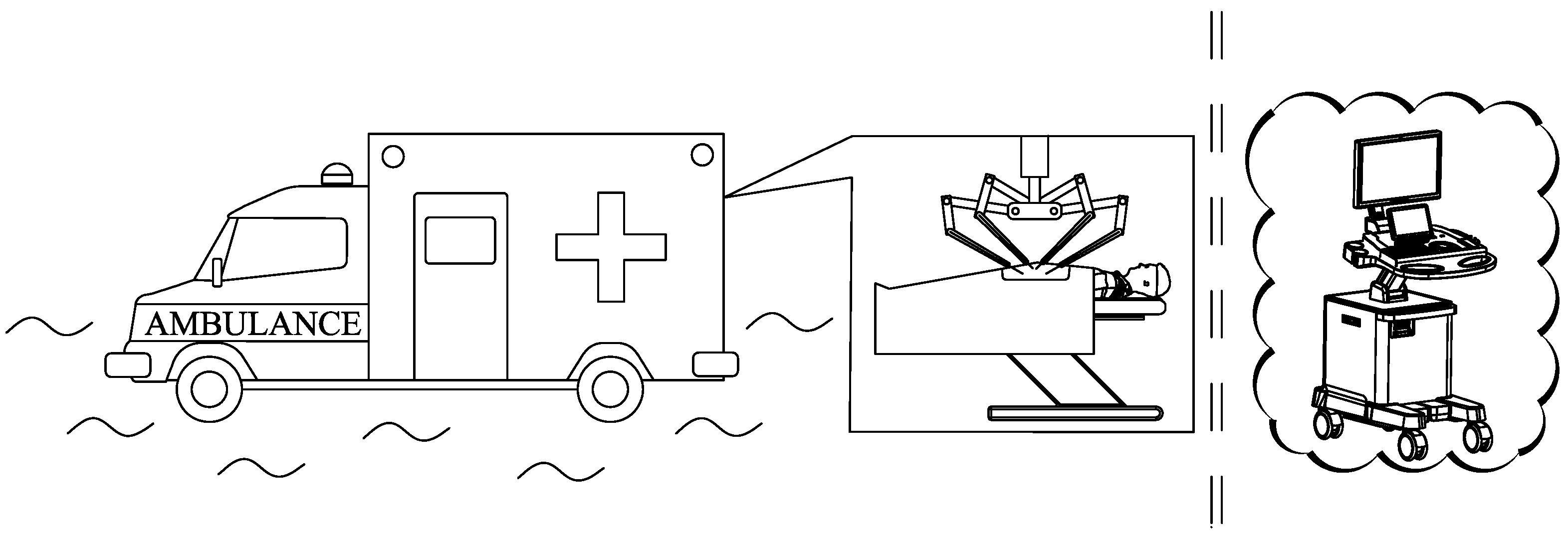
• Different from other OBMs, vehicle-mounted telesurgery manipulator operates in the non-inertial frame. This will lead to greater nonlinearity, and in turn bring more challenges to the control design.
• Most of current studies on OBMs do not consider the problems of input boundedness and payload uncertainty.

In order to address above problems, a novel stabilizing control method for vehicle-mounted telesurgery manipulator is proposed in this study. Compared with other robust control methods (such as $H_{\infty }$ control, slide mode control), this control has the following advantages.

• This control has a simpler structure and can be implemented more easily. It is actually a continuous varying-gain PD (proportional differential) control. However, $H_{\infty }$ control has the problem of high order, and is difficult to solve and implement in practice. High order slide mode control has similar problems, while low order one has chattering problem.
• The robust stability proof of proposed control is easier, due to control gains of which are related to a given implicit Lyapunov function [34].
• The proposed control also has boundary property that other controls do no have.

In summary, the main contributions of this study are as follows: As far as we know, this is the first control method that solves robust stabilizing problem of OBMs without predicting or measuring base oscillation. The robust asymptotic stability and boundary property of the control are proved theoretically. The hardware experimental system of vehicle-mounted manipulator considering real chassis oscillation is developed for the first time.

The rest of this paper is organized as follows. In Section 2, the problem statement as well as the dynamic model is described. In Section 3, the design process and stability analysis are presented. Section 4 provides the experimental implementation and results, and Section 5 gives concluding remarks of this paper.

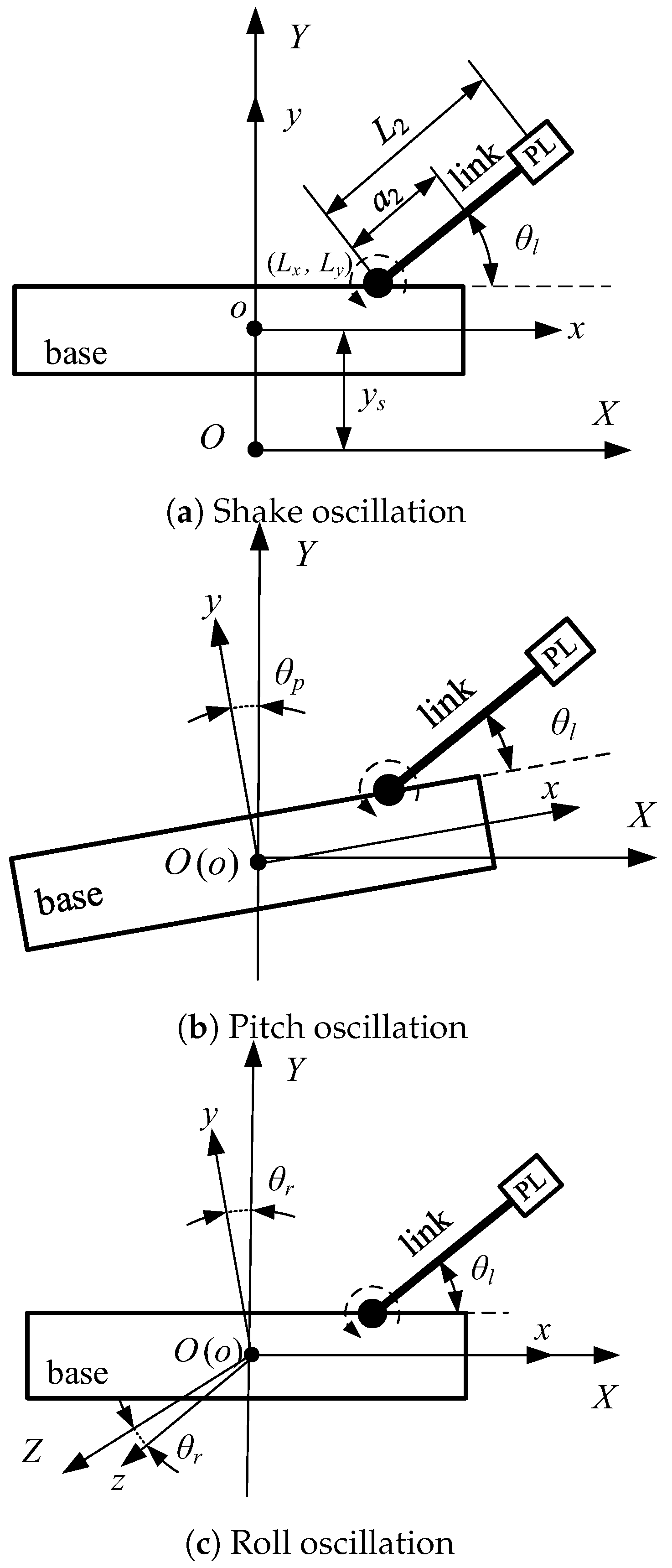
2. Problem Statements

For simplicity, we consider a simple OBMs system in the study as the first step of our long term research. The system is presented in Figure 2. As shown in the figure, the manipulator is a one-DOF (degree of freedom) link, the payload uncertainty is mass blocks at the end of the link, and base oscillations are divided into three parts: (i) shake oscillation, (ii) pitch oscillation, and (iii) roll oscillation. Figure 2a–c correspond to three oscillations, respectively.

Moreover, $OXYZ$ denotes the global frame; $oxyz$ is base-fixed frame; $y_s$, ${\theta }_p$ and ${\theta }_r$ denote shake, pitch and roll base oscillations, respectively; ${\theta }_l$ is link’s angular position; $L_2$ denote link length; $L_x$, $L_y$ is the position of link joint point; $a_2$ is the length between link’s centroid and joint point.

The dynamic model of above OBMs system is obtained using the Lagrangian formulation. Then, treating the base oscillations’ terms as external perturbations of manipulator, we obtain the following uncertain model:

$$J_e\ddot{q}+G\left(q\right)=U+S$$

(1)

where $q={\theta }_l$ is system state variable; $J_e$ is the equivalent moment of inertia; $G\left(q\right)$ denotes gravity force; U is link-side torque, namely, the control input needed to design; S is uncertain perturbation force caused by base oscillations. Moreover, $S=\left(S_s\mathrm{or}{S}_p\mathrm{or}{S}_r\right)$, where $S_s$, $S_p$ and $S_r$ denote shake, pitch and roll oscillations, respectively.

Each term of the equation is as following.

$$\begin{array}{cc}\hfill & J_e=J_2+J_{d2}+m_2{a}_2^2+m_{pl}{L}_2^2\hfill \\ \hfill & G\left(q\right)=(m_{2}g{a}_2+m_{pl}g{L}_2)\cos q\hfill \\ \hfill & S_s=-(m_2{a}_2+m_{pl}{L}_2)\cos q{\ddot{y}}_s\hfill \\ \hfill & S_p=-(J_2+m_2(a_2^2+L_x{a}_2\cos q+L_y{a}_2\sin q)+m_{pl}(L_2^2+L_x{L}_2\cos q+L_y{L}_2\sin q)){\ddot{\theta }}_p\hfill \\ \hfill & -(m_2(L_x{a}_2\sin q-L_y{a}_2\cos q)+m_{pl}(L_x{L}_2\sin q-L_y{L}_2\cos q)){\dot{\theta }}_p^2\hfill \\ \hfill & -((m_{2}g{a}_2+m_{pl}g{L}_2)\cos ({\theta }_p+q)-(m_{2}g{a}_2+m_{pl}g{L}_2)\cos q)\hfill \\ \hfill & S_r=m_2(a_2^2\sin q\cos q+L_y{a}_2\cos q){\dot{{\theta }_r}}^2+m_{pl}(L_2^2\sin q\cos q+L_y{L}_2\cos q){\dot{{\theta }_r}}^2\hfill \\ \hfill & -(m_2{a}_2+m_{pl}{L}_2)g(\cos q\cos {\theta }_r-\cos q)\hfill \end{array}$$

where $m_2$ denotes link mass, $J_2$ denotes its inertia moment with respect to the centroid; $J_{d2}$ is actuator inertia moment, usually negligibly small; $m_{pl}$ is payload mass; g denotes gravitational acceleration.

From the perspective of practical application, we assume that the following prerequisites hold for the system (1). These assumptions and property will facilitate the control system design and stability analysis [35].

A1. As mentioned before, the payload is uncertain, hence the system inertia $J_e$ is also uncertain. However, the payload uncertainty is assumed bounded in this study. Therefore, $J_e$ should satisfy the following condition:

$$J_{min}\le J_e\le J_{max}$$

(2)

where $J_{min}$ and $J_{max}$ are positive constants.

A2. The unknown term of S, including perturbations of not only chassis oscillations but also payload uncertainties, is also assumed bounded here.

$$\left|S\right|\le S_0,S_0>0$$

(3)

where $S_0$ is a positive constant.

A3. We also assume that there exist a positive constant $g_0$ such that

$$|\frac{\partial P\left(q\right)}{\partial q}|=|G\left(q\right)|\le g_0$$

(4)

where $P\left(q\right)$ is the gravitational potential energy of the system.

P1. Due to actuators saturates, the control input U should be bounded in practice. Hence, it has

$$\left|U\right|\le U_0,U_0>0$$

(5)

where $U_0$ is a positive constant.

Problem: The main problem faced in this study is to construct a controller U for system (1). It shall achieve the following performances: (i) robust stabilization of OBMs system against base oscillation; (ii) robustness to payload uncertainty; (iii) boundedness of control input.

Moreover, the following sub problems need to be considered in the controller design: (i) the determination of $S_0$ and $g_0$, which shall be estimated according to maximum allowable values of system state variables, base oscillation and payload uncertainty; (ii) the determination of $U_0$, which shall take in account not only $S_0$ but also actuators saturation.

3. Main Development

3.1. Constant PD Control

For system (1), if the uncertain pertubation $S=0$, an obvious choice for the control U is a constant-PD control plus gravity force compensation, namely,

$$\begin{array}{c}\hfill U=-k_d\dot{q}-k_{p}q+G\left(q\right)\end{array}$$

The PD gains, $k_p$ and $k_d$ could be easily obtained via classical tuning method, and the stability of the close-loop system could be proved via the Lassalle’s invariance theorem. However, in case that $S\ne 0$, the proof is no longer valid.

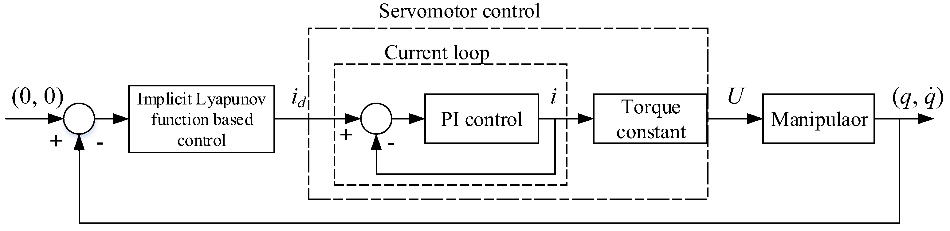
3.2. Implicit-Lyapunov-Function Based Control

In case that $S\ne 0$, for simplicity, the gravity-force term $G\left(q\right)$ is also regarded as one part of the perturbations. In particular, introduce a new notation $S^{\prime }=S-G$, Equation (1) could be rewritten as

$$J_e\ddot{q}=U+S^{\prime }$$

(6)

with

$$|S^{\prime }|\le S_0^{\prime },S_0^{\prime }=S_0+g_0$$

(7)

For the system (6), we redefine the controller U as

$$U=-k_d\dot{q}-k_{p}q$$

(8)

where

$$k_p=\frac{3{\beta }^2}{8V},k_d=\frac{\sqrt{3}\beta }{2\sqrt{2V{J}_{max}}}{J}_e$$

(9)

$$k_d^2=\frac{k_p{J}_e^2}{J_{max}}$$

(10)

$\beta >0$ is a constant, and V is a candidate Lyapunov function, as the following:

$$V(q,\dot{q})=\frac{1}{2}{J}_e{\dot{q}}^2+\frac{1}{2}{k}_p{q}^2+\frac{1}{2}{k}_{d}q\dot{q}$$

(11)

Obviously, $k_d$, $k_p$ and $V(q,\dot{q})$ are implicitly defined by Equations (9)–(11).

Next, we will prove the stability of the proposed close-loop control system using Lyapunov method. In other words, the positive-definiteness of $V(q,\dot{q})$, and the negative-definiteness of the derivative of V will be proved as the following.

Proof of Robust Stability. 

Introducing the notations

$$\begin{array}{c}\hfill x=V^{1/2},\xi =2\sqrt{2J_e}|\dot{q}|,\eta =\frac{2\sqrt{6}{U}_0{J}_e}{\sqrt{J_{max}}}q\dot{q},\gamma =\sqrt{3}{U}_0\left|q\right|\end{array}$$

(12)

where $\xi$, $\eta$ and $\gamma$ satisfying the conditions

$${\xi }^2+{\gamma }^2>0,\left|\eta \right|\le \left|\xi \gamma \right|$$

(13)

Then, substituting Equations (12) and (9) into Equation (11), an unary quartic equation will be obtained

$$16x^4-{\xi }^2{x}^2-\eta x-{\gamma }^2=0$$

(14)

For Equation (14), there is a theorem as following.

Theorem 1.

Every equation of the form

$$16x^4-{\xi }^2{x}^2-\eta x-{\gamma }^2=0$$

coefficients of which satisfy the inequality (13), has a unique positive real root and its multiplicity is one [36].

Due to $V=x^2$, we can conclude that V is also positive real, as well as $k_p$ and $k_d$.

Next, we will find the upper and lower bounds for V.

By Cauchy inequality and Equation (10), we can obtain

$$\begin{array}{cc}\hfill |k_{d}q\dot{q}|& =\sqrt{k_d^2{q}^2{\dot{q}}^2}=\sqrt{\frac{k_p{J}_e^2}{J_{max}}{q}^2{\dot{q}}^2}=\sqrt{\frac{k_p{J}_e}{J_{max}}{q}^2{J}_e{\dot{q}}^2}\hfill \\ \hfill & \le \sqrt{k_p{q}^2{J}_e{\dot{q}}^2}\le \frac{1}{2}{k}_p{q}^2+\frac{1}{2}{J}_e{\dot{q}}^2\hfill \end{array}$$

(15)

Furthermore, it has

$$\begin{array}{cc}\hfill & k_{d}q\dot{q}\ge -\frac{1}{2}{k}_p{q}^2-\frac{1}{2}{J}_e{\dot{q}}^2,k_{d}q\dot{q}\le \frac{1}{2}{k}_p{q}^2+\frac{1}{2}{J}_e{\dot{q}}^2\hfill \end{array}$$

(16)

Combining Equation (11) and inequality (16), it could be obtained the boundary of V

$$\begin{array}{c}\hfill \frac{1}{4}{k}_p{q}^2+\frac{1}{4}{J}_e{\dot{q}}^2\le V\le \frac{3}{4}{k}_p{q}^2+\frac{3}{4}{J}_e{\dot{q}}^2\end{array}$$

(17)

This also prove that V is always global positive definite for any $(q,\dot{q})\ne (0,0)$.

Furthermore, the value of the derivative of V will be evaluated.

Differentiating V along the trajectory (6) and (8), we have

$$\begin{array}{c}\hfill \dot{V}=J_e\dot{q}\ddot{q}+k_{p}q\dot{q}+\frac{1}{2}{k}_d{\dot{q}}^2+\frac{1}{2}{k}_{d}q\ddot{q}+\frac{1}{2}{\dot{k}}_p{q}^2+\frac{1}{2}{\dot{k}}_{d}q\dot{q}\end{array}$$

(18)

with

$$\begin{array}{c}\hfill \ddot{q}=\frac{1}{J_e}(U+S^{\prime })\end{array}$$

(19)

$$\begin{array}{c}\hfill {\dot{k}}_p=-\frac{k_p}{V}\dot{V}\end{array}$$

(20)

$$\begin{array}{c}\hfill {\dot{k}}_d=-\frac{1}{2}\frac{k_d}{V}\dot{V}\end{array}$$

(21)

By substituting Equations (19), (20) and (21) into Equation (18), we obtain

$$\begin{array}{c}\hfill \dot{V}\frac{1}{V}(\frac{1}{2}{J}_e{\dot{q}}^2+\frac{3}{4}{k}_{d}q\dot{q}+k_p{q}^2),=-\frac{k_d}{J_e}V+(\dot{q}+\frac{1}{2}{k}_d\frac{1}{J_e}q)S^{\prime }\end{array}$$

(22)

By introducing a new notation B

$$\begin{array}{c}\hfill B=\frac{1}{V}(\frac{1}{2}{J}_e{\dot{q}}^2+\frac{3}{4}{k}_{d}q\dot{q}+k_p{q}^2)\end{array}$$

(23)

then the Equation (23) could be rewritten as

$$B\dot{V}=-\frac{k_d}{J_e}V+(\dot{q}+\frac{1}{2}{k}_d\frac{1}{J_e}q)S^{\prime }$$

(24)

Moreover, according to inequality (16), B can be written as

$$\begin{array}{c}\hfill B\ge \frac{1}{V}(\frac{1}{2}{J}_e{\dot{q}}^2+k_p{q}^2+\frac{3}{4}(-\frac{1}{2}{k}_p{q}^2-\frac{1}{2}{J}_e{\dot{q}}^2))=\frac{1}{V}(\frac{1}{8}{J}_e{\dot{q}}^2+\frac{5}{8}{k}_p{q}^2)\end{array}$$

(25)

It is obvious that B is always positive for any $(q,\dot{q})\ne (0,0)$. Hence, to prove the positive-definiteness of $\dot{V}$, we only need to prove the value of the right side of (24) are negative.

By substituting Equation (10) into the second term of the right side of (24), it can be obtained

$$\begin{array}{c}\hfill {(\dot{q}+\frac{1}{2}{k}_d\frac{1}{J_e}q)}^2=\frac{1}{J_e}(J_e{\dot{q}}^2+\frac{1}{4}{J}_e\frac{k_p}{J_{max}}{q}^2+k_{d}q\dot{q})\end{array}$$

(26)

According to the assumption A1, Equation (26) could be further rewritten

$$\begin{array}{c}\hfill {(\dot{q}+\frac{1}{2}{k}_d\frac{1}{J_e}q)}^2\le \frac{1}{J_e}(J_e{\dot{q}}^2+\frac{1}{4}{k}_p{q}^2+k_{d}q\dot{q})\le \frac{2}{J_e}V\end{array}$$

(27)

Combining (27) and (7), we obtain

$$\begin{array}{c}\hfill (\dot{q}+\frac{1}{2}{k}_d\frac{1}{J_e}q)S^{\prime }\le \sqrt{\frac{2}{J_e}V}{S}_0^{\prime }\end{array}$$

(28)

Then, substituting inequality (28) into Equation (24), it has

$$\begin{array}{c}\hfill \dot{V}\le -\frac{1}{B}(\frac{k_d}{J_e}V-\sqrt{\frac{2}{J_e}V}{S}_0^{\prime })\end{array}$$

(29)

By substituting the expression of $k_d$ into (29), it further has

$$\begin{array}{c}\hfill \dot{V}\le -\frac{1}{B}\sqrt{V}(\frac{\sqrt{3}\beta }{2\sqrt{2J_{max}}}-\sqrt{\frac{2}{J_e}}{S}_0^{\prime })\end{array}$$

(30)

Obviously, to prove the negative-definiteness of $\dot{V}$, the following condition should be satisfies

$$\begin{array}{c}\hfill \beta \ge \frac{4}{3}\sqrt{\frac{3J_{max}}{J_e}}{S}_0^{\prime }\end{array}$$

(31)

Furthermore,

$$\begin{array}{c}\hfill \beta \ge \frac{4}{3}\sqrt{\frac{3J_{max}}{J_e}}(S_0+g_0)\end{array}$$

(32)

So far we have proved the positive definiteness of the Lyapunov function $V\left(q,\dot{q}\right)$ and the negative definiteness of its differential function along trajectories of system (6). By Lassalle’s invariance theorem, it could be concluded that the equilibrium state of system (6), $(q,\dot{q})=(0,0)$, is globally asymptotically stable.

Moreover, from Equations (30) and (31), we can conclude that there is a constant $\alpha >0$ such that

$$\dot{V}(q,\dot{q})\le -\alpha V(q,\dot{q})$$

(33)

for all $(q,\dot{q})$. This implies that the above control system is global exponential stability.

From the expressions of $k_p$ and $k_d$, it can be found that the gains approach to infinity as the Lyapunov function tends to zero. However, the control forces should be bounded in practice, and satisfy the given condition (4). □

Next, we will prove the bound property of the control input (8).

Proof of Bounded property.

According to Equation (8) and Cauchy inequality, we obtain

$$\begin{array}{c}\hfill U^2=k_d^2{\dot{q}}^2+k_p^2{q}^2+2k_d{k}_{p}q\dot{q}\le \frac{4}{3}(k_d^2{\dot{q}}^2+k_p^2{q}^2+k_p{k}_{d}q\dot{q})\end{array}$$

(34)

Then, substituting Equations (10) and (11) into Equation (34), it has

$$\begin{array}{c}\hfill U^2\le \frac{4}{3}(\frac{k_p{J}_e^2}{J_{max}}{\dot{q}}^2+k_p^2{q}^2+k_d{k}_{p}q\dot{q})\le \frac{4}{3}(k_p{J}_e{\dot{q}}^2+k_p^2{q}^2+k_d{k}_{p}q\dot{q})=\frac{8}{3}{k}_{p}V={\beta }^2\end{array}$$

(35)

It is clear that the control input is limited by the parameter $\beta$. By setting $U_0=\beta$, the property P1 will been obtained. □

4. Performance Evaluation

To verify the performance of the proposed control, we developed an experimental platform, which is corresponding to the OBM model in Figure 2a. Moreover, before the hardware experiments, we firstly carried out simulations as a preliminary work of the hardware experiments.

4.1. System Development

Before developing the hardware experiment platform, a virtual prototype system is firstly constructed. It is shown in Figure 3. The system consists of a one-link manipulator, a mounted frame (the oscillatory base), spring-tracks and a fixed base. The manipulator together with the mounted frame can oscillate along the tracks under external excitations. The spring is used to simulate the role of the vehicle shock absorber. The manipulator is actuated by a DC motor, and the motor is driven by the computer instructions through a digital position controller.

The system parameters are: $J_2=0.009\mathrm{kg}·{\mathrm{m}}^2$, $m_2=1.38\mathrm{kg}$, $a_2=0.14\mathrm{m}$, $L_2=0.26\mathrm{m}$. The equivalent value of $J_{d2}$ is included in $J_2$. For simplicity, we set $L_x=L_y=0$. The control parameters are set as: $U_0=15\mathrm{Nm}$, $J_{max}=0.1$.

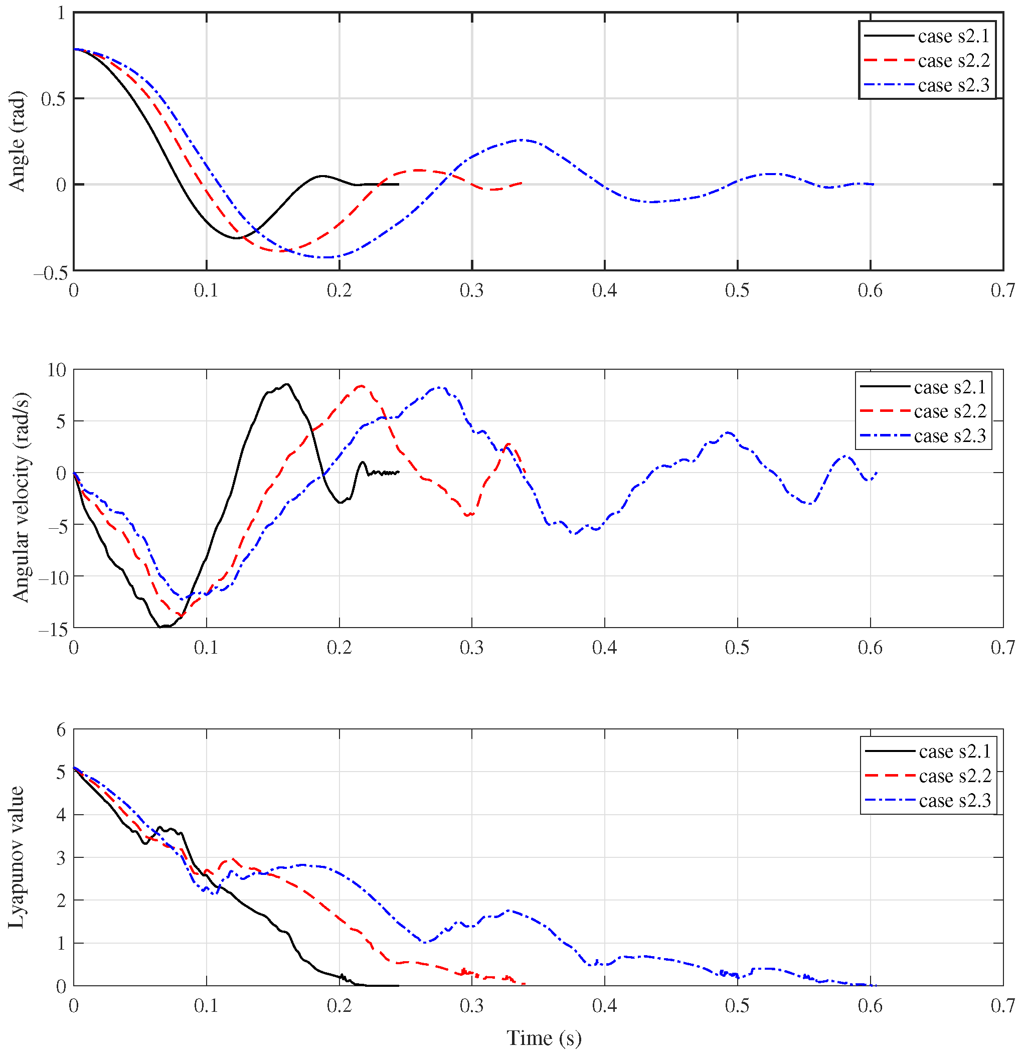
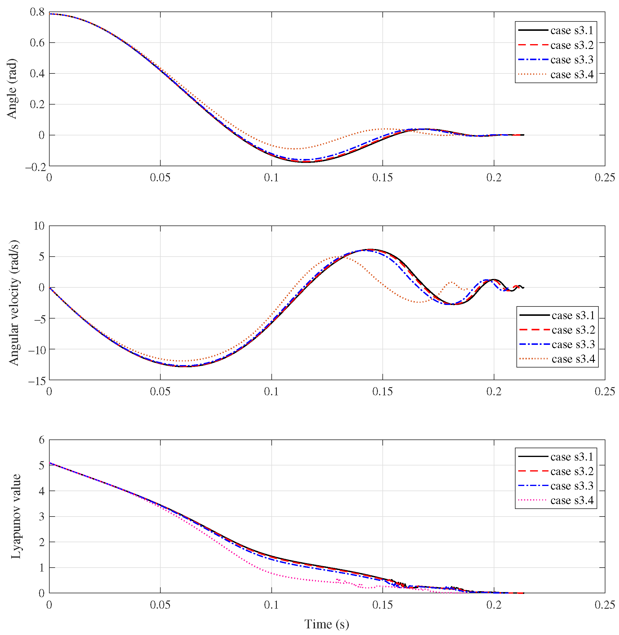
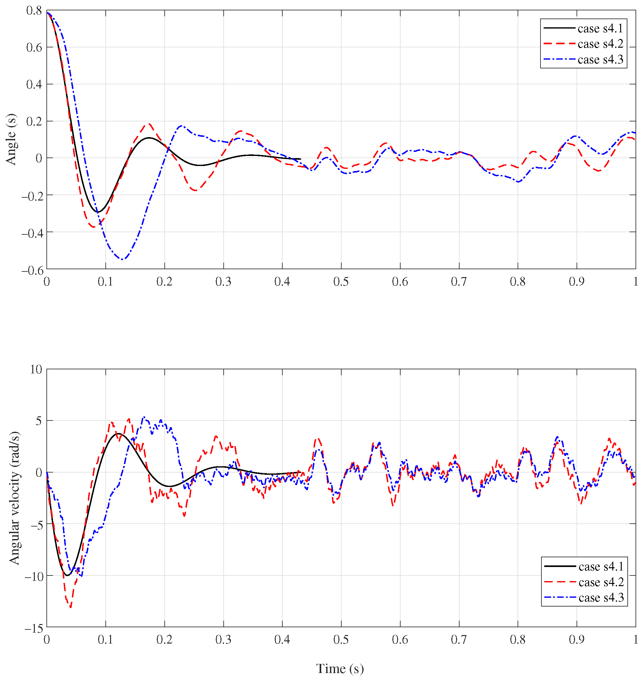
4.2. Simulations and Result Analysis

Four groups of simulations were carried out in MATLAB. As shown in

Table 1. Simulation groups.

Group NO.	Case NO.	Control	Oscillation		Payload
Group s1	case s1.1	IL PD	shake	real	0 kg
	case s1.2	IL PD	pitch	real	0 kg
	case s1.3	IL PD	roll	real	0 kg
	case s1.4	IL PD	no		0 kg
Group s2	case s2.1	IL PD	pitch	real	0 kg
	case s2.2	IL PD	pitch	real	0.4 kg
	case s2.3	IL PD	pitch	real	0.8kg
Group s3	case s3.1	IL PD	pitch	$5^{\circ }$ sin($\pi$t)	0 kg
	case s3.2	IL PD	pitch	${10}^{\circ }$ sin($\pi$t)	0 kg
	case s3.3	IL PD	pitch	${20}^{\circ }$ sin($\pi$t)	0 kg
	case s3.4	IL PD	pitch	${20}^{\circ }$ sin(2$\pi$t)	0 kg
Group s4	case s4.1	PD	no		0 kg
	case s4.2	PD	pitch	real	0 kg
	case s4.3	PD	pitch	real	0.8 kg

, the Group s1 simulation is used to certify the proposed control’s robustness against to real base oscillations. These oscillations are from our previous studies of the vehicles maneuverability simulation in ADAMS/ATV software. The Group s2 is used to further certify the control’s robustness against to payload uncertainties. The Group s3 is to verify the control’s performance against to traditional base oscillations, which is usually formulated as ${\theta }_l=Asin\left(\omega t\right)$. Moreover, another group of simulations with traditional PD control used for comparison is carried out in Group s4.

The IL PD in the table means the proposed implicit Lyapunov control. The PD means traditional PD control with constant gains. The gains are set as $k_p=12.9904$ and $k_d=0.4109$, respectively. In addition, for simplicity, we account for only the pitch oscillation in the simulation of Group s2, s3 and s4.

Group s1: Four cases of simulations are carried out in this group. The case s1.1, s1.2 and s1.3 correspond to the case of shake, pitch and roll oscillation, respectively. The case s1.4 is a contrast one, where no oscillation is considered.

The simulation results are presented in Figure 4. The red dash line, black solid line, blue dash-dot line and orange dot line describe the simulation results of the case s1.1, s1.2, s1.3 and s1.4 respectively.

The upper subfigure describes the angular trajectory of the manipulator, the middle one is the angular velocity of which. The manipulator system was brought from the initial state ($q={45}^{\circ },\dot{q}=0$) to the horizontal position ($q=0,\dot{q}=0$) in a very short time. The setting time for four cases are 0.265 s, 0.245 s, 0.216 s and 0.216 s, respectively. Obviously, the shake oscillation has the greatest effect on the system response in almost all performance index, not only the setting time but also the overshoot, et al. The roll oscillation has very little effect, the curves of which are nearly overlapped with the case of no oscillation. It can also been found that the shake oscillation and pitch oscillation causing a non-smooth characteristic of the angular velocity curve.

The lower subfigure depicts the time history of the Lyapunov function V along the system trajectory. It can been seen that the Lyapunov function curve for the case of roll and no oscillation is decreasing monotonically, but for the case of shake and pitch oscillation it is not. This is because that the setting of $U_0$ depends on the value of $S_0$, but the value is not easily to confirmed in practice. A simple estimating value is selected in this study. Nonetheless, the proposed controller still demonstrated good robustness to real oscillations.

Group s2: Two more cases of simulations are carried out in this group. The case s2.2 and s2.3 correspond to the case of payload uncertainty equal to 0.4 kg and 0.8 kg, respectively. The case s2.1, which is actually the case s1.2 in the Group s1, is regarded as a contrast case with nominal inertia in this group. In addition, as mentioned above, only the pitch oscillation is considered here.

The simulation results are presented in Figure 5. The black solid line corresponds to the case s2.1, the red dash line corresponds to the case s2.2, and the blue dash-dot line corresponds to the case s2.3.

Similarly, the upper two subfigures illustrate the motion response of the manipulator system: angular coordinate and velocity. The system was steered to the terminal state from the given initial state in finite time. It takes 0.245 s, 0.340 s and 0.605 s for the case of 0 kg, 0.4 kg and 0.8 kg, respectively. Clearly, the bigger the payload uncertainty, the longer the setting time. The increase of the payload uncertainty will also bring about the increase of the overshoot.

Moreover, the lower subfigure presents the behaviour of the function V along the system trajectory. Due to the payload uncertainties was not considered when selecting the parameter of $S_0$, the Lyapunov curves of these cases show more significant nonmonotonical characteristics. However, the controller still show good robustness to both base oscillations and payload uncertainties.

Group s3: This group carried out four more cases of simulations, where four sinusoidal pitch oscillations with different amplitude/frequency are considered. Specially, the amplitude/frequency of case s3.1, s3.2 s3.3 and s3.4 are $5^{\circ }/\pi$, ${10}^{\circ }/\pi$, ${20}^{\circ }/\pi$, and ${20}^{\circ }/2\pi$, respectively.

Figure 6 shows the simulation results. The black solid line, red dash line, blue dash-dot line and orange dot line correspond to the case s3.1, s3.2 s3.3 and s3.4, respectively.

The upper two subfigures show clearly the point-to-point motion of the manipulator system. The setting time are 0.213 s, 0.214 s, 0.207 s and 0.189 s for the case s3.1, s3.2 and s3.4, respectively. It can been seen that the increase of the amplitude has little effect on the system response, but the changing of the frequency greatly reduce the setting time. It can also been found that both the angle and angular velocity curves are smooth in the whole process. Moreover, the lower subfigure shows that the trajectory of Lyapunov function V is roughly monotonically decreasing.

In summary, we can conclude that the proposed control has good performance against to not only real oscillation but also sinusoid oscillation. Moreover, the control’s performance remain under the varying of the oscillation in amplitude and frequency.

Group s4: This contrast group includes three more cases of simulations. For these simulations, the PD with gravity compensation is used. Moreover, the case s4.1 does not consider the base oscillation nor the payload uncertainty. The case s4.2 only considers real pitch oscillation, and the case s4.3 further takes into account the payload uncertainty.

The motion response of the manipulator system is presented in Figure 7. The black solid line, red dash line and blue dash-dot line are corresponding to the results of case 4.1, 4.2 and 4.3, respectively.

It is clear that the controller can achieve the stabilization of the system without base oscillations and payload uncertainties. It steers the manipulator from the initial state to the equilibrium state in 0.265 s. However, under the influence of base oscillations and payload uncertainties, the controller lost it’s performance. The system is no longer stable. Both the angle and angular velocity curves exhibit obviously oscillating feature.

The control input U as a function of time is presented in Figure 8. The upper, middle and lower subfigures correspond to the Group s1, s2, and s3, respectively. It is clear that the control U satisfies the restriction $U\le U_0$ in all simulations. Hence, it is a kind of boundary control method. In addition, the Figure 9 presents the real shake, pitch and roll oscillation, respectively.

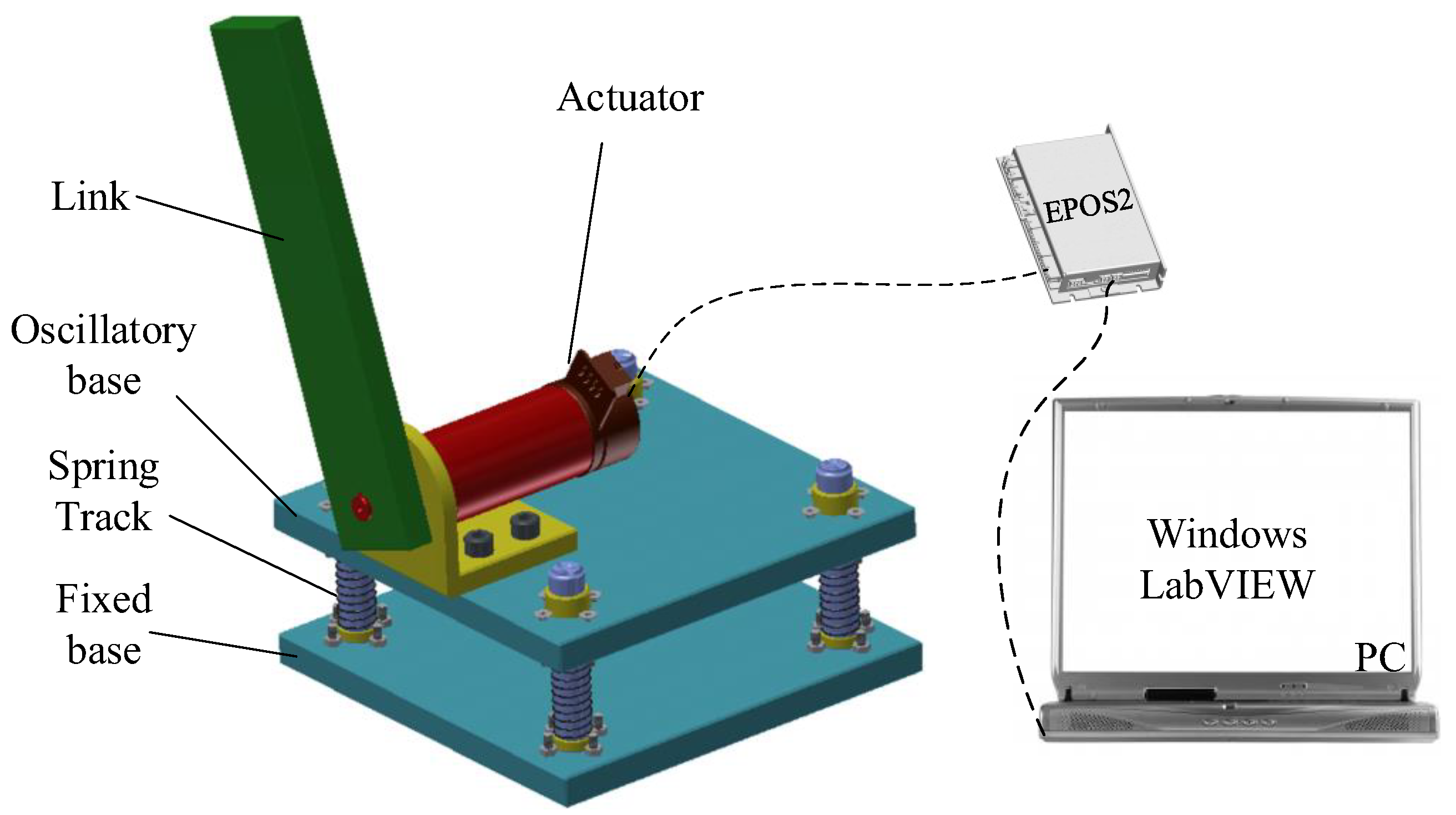
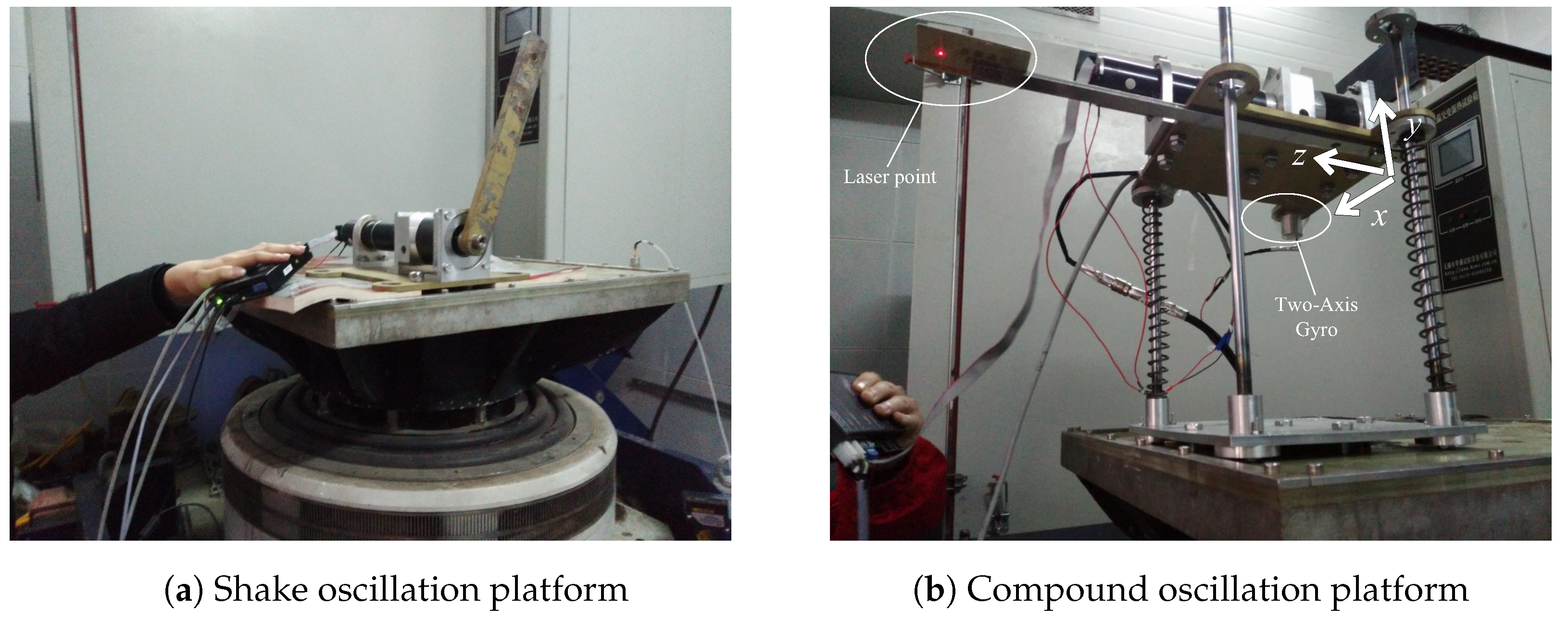
4.3. Hardware Configurations

Based on above virtual prototype system and simulations, we developed the following hardware platform, as shown in Figure 10. Similarly, it also includes a one-link manipulator, a mounted frame, a spring-track system and a fixed frame. The manipulator is actuated by a Maxon-RE50 motor through two reducers (Maxon, GP52C and YINGTONG DRIVE, PF90-3, respectively). Moreover, the motor is equipped with a digital encoder (Maxon HEDL 5540) in the rear to measure the motor rotational motion.

For simplicity, we firstly carried out the experiments considering only shake oscillations. The manipulator system is directly mounted on an electromagnetic vibration table, as shown in Figure 10a. The vibration table, provided by ETS Solution Beijing Ltd., is able to generate various of shake oscillations as required. Moreover, further experiments, which take in account the shake, pitch and roll oscillations simultaneously, were carried out. The hardware platform is shown in Figure 10b. The manipulator together with the frame and the spring-track are mounted on the vibration table. We call this oscillation as the compound oscillation in this study. In addition, a two-axis gyroscope is used to measure the pitch oscillation (velocity along z-axis) and roll oscillation (velocity along x-axis). A laser sensor is used to measure the shake oscillation (position along y-axis).

For the control hardware system, we adopted a digital positioning controller (MAXON EPOS2) together with a personal computer, as shown in Figure 3. The master-slave technique is used for the hardware communication. The controller communicates as a slave, and the computer communicates as a master. The data transition between PC and controller is based on the USB-serial-port communication protocol.

The EPOS2 controller has a build-in control loop. It is a kind of three-loop control method, which consists of a current loop, a position loop and a velocity loop. For our experiments here, the embedded current-loop is adopted, but the position-velocity loop is replaced by our self-build control loop. The current-loop uses the proportional-integral control. The position-velocity loop is a real-time program of the proposed implicit-Lyapunov control. The program is developed in the LabVIEW software. The two control loops are connected by the torque constant of the motor, as shown in Figure 11. Due to the linear relationship between the torque and current of the motor, we can conclude that the desired current of the motor must satisfy the following condition.

$$\left|c_{desired}\right|\le c_0,c_0=\frac{i{U}_0}{C_t}$$

(36)

where $C_t$ is the torque constant of the motor, i is the transmission ratio of the system.

In addition, the sampling frequency of the current, position and velocity are 10 kHz, 1 kHz and 1 kHz, respectively.

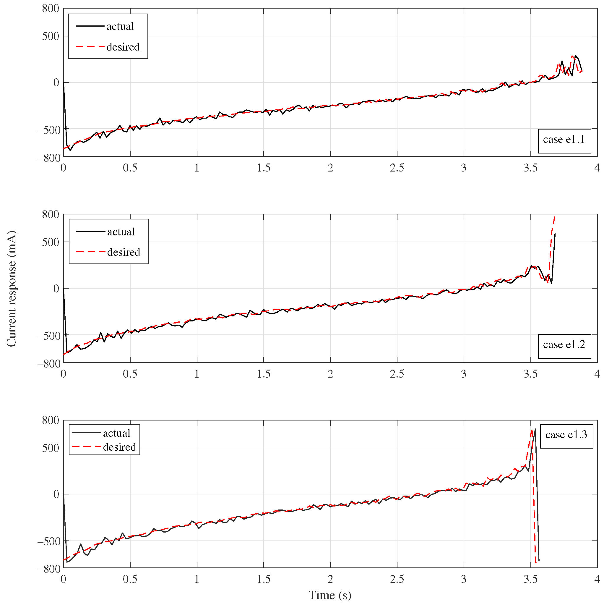
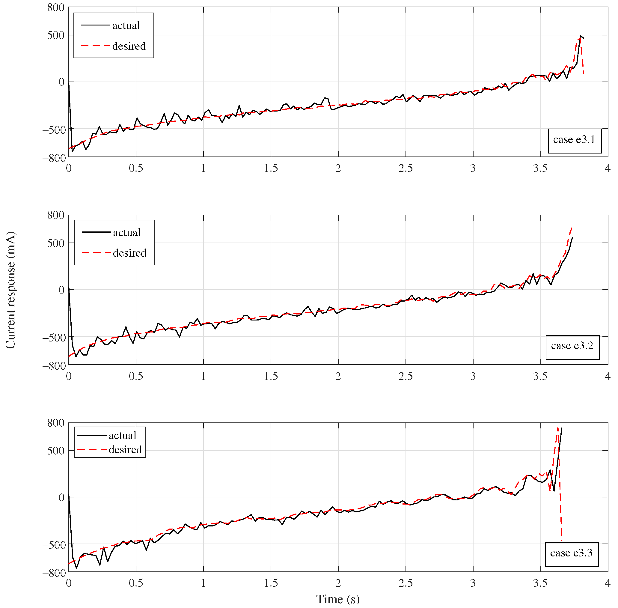
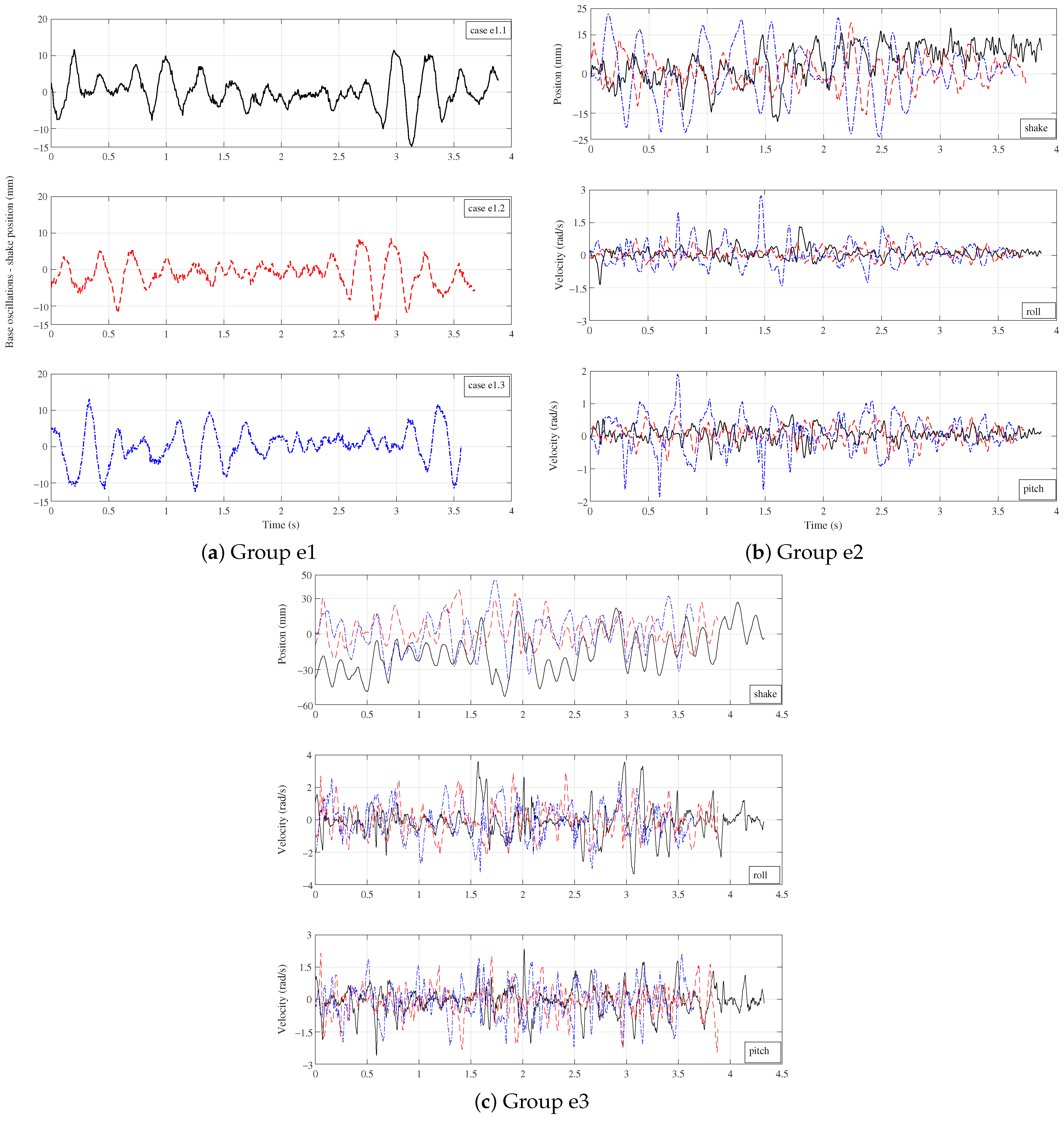
4.4. Experiment Results and Analysis

Four groups of experiments were carried out based on above hardware platform, as shown in

Table 2. Experiment groups.

Group NO.	Case NO.	Oscillation		Payload
Group e1	case e1.1	shake	real	0 kg
	case e1.2	shake	real	0.4 kg
	case e1.3	shake	real	0.8 kg
Group e2	case e2.1	shake	sinusoidal	0 kg
	case e2.2	shake	sinusoidal	0.4 kg
	case e2.3	shake	sinusoidal	0.8kg
Group e3	case e3.1	Compound	real	0 kg
	case e3.2	Compound	real	0.4 kg
	case e3.3	Compound	real	0.8 kg
Group e4	case e4.1	Compound	sinusoidal	0 kg
	case e4.2	Compound	sinusoidal	0.4 kg
	case e4.3	Compound	sinusoidal	0.8 kg

. The Group e1/e2 experiments are based on the left platform (Figure 10a), and the Group e3/e4 are based on the right platform (Figure 10b). For the two platforms, both the real and sinusoidal excitation are applied to the vibration table. Specially, the Group e1, e2, e3 and e4 are corresponding to real shake, sinusoidal shake, real compound and sinusoidal compound oscillation, respectively. Similar with the simulations, the real excitation is from our previous study. The amplitude and frequency of the sinusoidal excitation are set as: 10 mm and 36 rad/s, respectively.

The system parameters for above experiments are the same as the simulations. The initial and terminal state of the manipulator system are also the same: $(q_0,{\dot{q}}_0)=({45}^{\circ },0)$, $(q_{*},{\dot{q}}_{*})=(0^{\circ },0)$. Moreover, the boundedness of the motor current is $c_0=805$ mA. The control gains of the current loop are set as: $k_p=335$ and $k_I=115$, respectively.

Group e1: In this group, we carried out three cases of experiments. The case e1.1 considers the base oscillation only, the case e1.2 and e1.3 further takes into account the payload uncertainties, 0 kg, 0.4 kg and 0.8 kg, respectively.

The experiment results are shown in Figure 12 and Figure 13. The upper two subfigures of Figure 12 present the motion responses of the manipulator. The black solid line, red dash line and blue dash-dot line correspond to the case e1.1, e1.2 and e1.3, respectively. It is clear that the control successfully steer the system to its equilibrium point in short time. The setting time are 3.884 s, 3.683 s and 3.562 s for the three cases, respectively. It can also been found that it takes less time for the case of payload uncertainty than the case of no payload. The bigger the payload uncertainty, the less the setting time. This is because that the angular trajectory of the manipulator tends to the terminal state in a monotonically-decreasing way. The gravity force always plays an active role during the falling of the manipulator. Similar with the simulations, the angular velocity curves also exhibit non-smooth feature.

The lower subfigure of Figure 12 show the time history of the function V. It is clear that V is is strictly monotonic decreasing for all three cases. Figure 13 presents the current responses. The black solid line and the red dash line corresponds to the actual motor current and computed desired current, respectively.

The motor current approaches to its desired value in a very short time for all three cases. The current for the case of payload uncertainty are bigger than the case of no payload. Moreover, it can been seen that the current gets large near the end of the trajectory. This is because that the Lyapunov function appears in the denominator of the control gains, and the gains will increase to infinity as the manipulator system tends to the equilibrium. However, there is no need to bring a system to the $(0,0)$ point in practice. When the Euclidean distance between the actual state and the terminal state fell below a certain value, it already meets the accuracy requirements. We set this value as 0.01 here. In addition, it clear that the control input satisfies the given constraints. It remains bounded in norm during the whole process.

Group e2: Similarly, this group also carried out three cases of experiments with three different payload uncertainties. The sinusoid shake base oscillation is considered.

The experiments are presented in Figure 14 and Figure 15. Specially, Figure 14 shows the system response. The black solid line, red dash line and blue dash-dot line correspond to the case e2.1, e2.2 and e2.3, respectively. Figure 15 shows the current response. The black solid line is the actual motor current, and the red dash line is the computed desired current.

From the upper two subfigures of Figure 14, it can been seen that the manipulator is steered from the given state to the terminal state in short time. The setting time for the case e2.1, e2.2 and e2.3 are 3.81 s, 3.56 s and 3.23 s, respectively. Similar with the Group e1, the bigger the payload uncertainty, the less the setting time. The reason is the same as the Group e1. We can also find that the angular velocity curves of this group exhibit more obviously oscillating feature than the Group e1.

The lower subfigure of Figure 14 shows the time history of the Lyapunov function. It is strictly monotonic decreasing.

From Figure 15, it can been seen that the PI control used in the current-loop has good trajectory tracking performance. The actual motor current can track the desired current quickly and stably. Moreover, it can also been found that the current curves of this group exhibit more obviously oscillating feature than the Group e1. Nonetheless, it still satisfies the boundedness properties in the whole process.

Group e3: This group carried out three more experiments. The real compound oscillation and three different payload uncertainties are considered.

The simulation results are presented in Figure 16 and Figure 17. Figure 16 illustrates the system response. The black solid line corresponds to the case e3.1, and the red dash line case e3.2, the blue dash-dot line the case e3.3.

The upper subfigure of Figure 16 depicts the angular trajectory of the manipulator, the middle one presents the angular velocity curves. It is clear that the control has achieved the accuracy positioning control of the manipulator. It steers the system arriving at the equilibrium point in 3.872 s, 3.737 s and 3.663 s, respectively. It can also been seen that the angular velocity curves are still non-smooth. Moreover, the lower subfigure shows the time history of the monotonic decreasing function V.

Figure 17 illustrates the current response. The black solid line depicts the actual motor current, and the red dash line the computed value of the desired current. It can been seen that the actual current catch up with the desired current in very short time. Additionally, it can also been found that the current curves of this group exhibit more obviously oscillating feature than Group e1 and e2.

Group e4: This group further carried out three experiments, where three different payload uncertainties together with the sinusoid compound oscillation are considered.

The system response and current response are shown in Figure 18 and Figure 19, respectively. Similarly, the black solid line, red dash line and blue dash-dot line in Figure 18 correspond to the case e4.1, e4.2 and e4.3, respectively. The black solid line and red dash line in Figure 19 depicts the actual and desired current, respectively.

The upper two subfigures of Figure 18 illustrate the time history of the motion of the manipulator, and the lower one illustrates that of the function V. The system arrives at the terminal state in 4.328s, 3.881s and 3.65s for three cases, which the function V monotonically decreases to zero. Moreover, the Figure 19 proves good tracking performance of the the current control and boundary characteristic of the proposed control. In addition, the base oscillation responses for above experiments are presented in Figure 20. Specially, the upper, middle and lower subfigure correspond to the Group e1, e3 and e4, respectively. The blue dotted line, the red dash-dotted line and the black solid line denote the case of no payload, 0.4 kg payload and 0.8 kg payload, respectively.

5. Conclusions

This paper proposed a novel positioning control strategy for a novel OBM system that is subject to not only base-oscillation-induced disturbance but also the problem of payload uncertainty and actuator saturation. Based on the simulation and experiment results, we can conclude that the proposed control has good robustness to both base oscillation and payload uncertainty, and can achieve accuracy positioning of the OBM without the prediction or measurement of the base oscillation. Moreover, the suggested control’s boundedness has also been demonstrated both theoretically and in simulation/experiment studies. This research also has implications for enhancing other OBMs’ ability to control motion. However, the proposed control has only been applied to a simple OBM system. The base oscillation circumstances and actual OBM system are undoubtedly more intricate. In future research, we will devote more effort to investigate the efficacy of the proposed controls on real complex systems.

References

1. Toda, M. Robust Motion Control of Oscillatory-Base Manipulators, 1st ed.; Springer International Publishing: Cham, Switzerland, 2016; pp. 7–9. [Google Scholar]
2. Zhang, Y.; Liu, Y.; Xie, Z.; Liu, Y.; Cao, B.; Liu, H. Visual servo control of the macro/micro manipulator with base vibration suppression and backlash compensation. Appl. Sci. 2022, 12, 8386. [Google Scholar] [CrossRef]
3. Palma, P.; Seweryn, K.; Rybus, T. Impedance control using selected compliant prismatic joint in a free-floating space manipulator. Aerospace 2022, 9, 406. [Google Scholar] [CrossRef]
4. Zhang, S.; Cheng, S.; Jin, Z. A control method of mobile manipulator based on null-space task planning and hybrid control. Machines 2022, 10, 1222. [Google Scholar] [CrossRef]
5. González-García, J.; Narcizo-Nuci, N.A.; Gómez-Espinosa, A.; García-Valdovinos, L.G.; Salgado-Jiménez, T. Finite-time controller for coordinated navigation of unmanned underwater vehicles in a collaborative manipulation task. Sensors 2023, 23, 239. [Google Scholar] [CrossRef] [PubMed]
6. Martin-Abadal, M.; Oliver-Codina, G.; Gonzalez-Cid, Y. Real-time pipe and valve characterisation and mapping for autonomous underwater intervention tasks. Sensors 2022, 22, 8141. [Google Scholar] [CrossRef]
7. Cao, Y.; Li, T.; Hao, L. Nonlinear model predictive control of shipboard boom cranes based on moving horizon state estimation. J. Mar. Sci. Eng. 2023, 11, 4. [Google Scholar] [CrossRef]
8. Chen, M.; Yuan, G.; Li, C.B.; Zhang, X.; Li, L. Dynamic analysis and extreme response evaluation of lifting operation of the offshore wind turbine jacket foundation using a floating crane vessel. J. Mar. Sci. Eng. 2022, 10, 2023. [Google Scholar] [CrossRef]
9. Guo, Y.; Hou, B. Implicit Lyapunov function-based tracking control of a novel ammunition autoloader with base oscillation and payload uncertainty. Nonlinear Dyn. 2017, 87, 741–753. [Google Scholar]
10. Guo, Y.; Xi, B.; Huynh, V.T.; Wang, Z. Robust tracking control of MBT autoloaders with oscillatory chassis and compliant actuators. Nonlinear Dyn. 2019, 99, 2185–2200. [Google Scholar] [CrossRef]
11. Wang, S.; Yang, Y.; Li, G.; Du, H.; Wei, Y. Microscopic vibration suppression for a high-speed macro-micro manipulator with parameter perturbation. Mech. Syst. Signal Process. 2022, 179, 109332. [Google Scholar] [CrossRef]
12. Yang, Y.; Wei, Y.; Lou, J.; Fu, L.; Fang, S.; Chen, T. Dynamic modeling and adaptive vibration suppression of a high-speed macro-micro manipulator. J. Sound Vib. 2018, 442, 318–342. [Google Scholar] [CrossRef]
13. Chen, T.; Lou, J.; Yang, Y.; Ren, Z.; Xu, C. Vibration suppression of a high-speed macro-micro integrated system using computational optimal control. IEEE Trans. Ind. Electron. 2020, 67, 7841–7850. [Google Scholar] [CrossRef]
14. Park, H.C.; Chakir, S.; Kim, Y.B.; Lee, D.H. A robust payload control system design for offshore cranes: Experimental study. Electronics 2021, 10, 462. [Google Scholar] [CrossRef]
15. Qian, Y.; Fang, Y. Switching logic-based nonlinear feedback control of offshore ship-mounted tower cranes: A disturbance observer-based approach. IEEE Trans. Autom. Sci. Eng. 2019, 16, 1–12. [Google Scholar] [CrossRef]
16. Wang, Y.; Wang, S.; Wei, Q.; Tan, M.; Zhou, C.; Yu, J. Development of an underwater manipulator and its free-floating autonomous operation. IEEE ASME Trans. Mechatron. 2016, 21, 815–824. [Google Scholar] [CrossRef]
17. Xue, G.; Liu, Y.; Shi, Z.; Guo, L.; Li, Z. Research on trajectory tracking control of underwater vehicle manipulator system based on model-free adaptive control method. J. Mar. Sci. Eng. 2022, 10, 652. [Google Scholar] [CrossRef]
18. Toda, M. An H control-based approach to robust control of mechanical systems with oscillatory bases. IEEE Trans. Rob. Autom. 2004, 20, 283–296. [Google Scholar] [CrossRef]
19. Londhea, P.S.; Mohanb, S.; Patrea, B.M.; Waghmarea, L.M. Robust task-space control of an autonomous underwater vehicle manipulator system by PID-like fuzzy control scheme with disturbance estimator. Ocean Eng. 2017, 139, 1–13. [Google Scholar] [CrossRef]
20. Cai, Y.; Zheng, S.; Liu, W.; Qu, Z.; Zhu, J.; Han, J. Sliding-mode control of ship-mounted Stewart platforms for wave compensation using velocity feedforward. Ocean Eng. 2021, 236, 109477. [Google Scholar] [CrossRef]
21. Sato, M.; Toda, M. Robust motion control of an oscillatory-base manipulator in a global coordinate system. IEEE Trans. Ind. Electron. 2015, 62, 1163–1174. [Google Scholar] [CrossRef]
22. Leban, F.A.; Diaz-Gonzalez, J.; Parker, G.G.; Zhao, W. Inverse kinematic control of a dual crane system experiencing base motion. IEEE Trans. Control Syst. Technol. 2015, 23, 331–339. [Google Scholar] [CrossRef]
23. Sun, N.; Fang, Y.; Chen, H.; Fu, Y.; Lu, B. Nonlinear stabilizing control for ship-mounted cranes with ship roll and heave movements: Design, analysis, and experiments. IEEE Trans. Syst. Man Cybern. 2018, 48, 1781–1793. [Google Scholar] [CrossRef]
24. Sun, N.; Yang, T.; Chen, H.; Fang, Y. Dynamic feedback antiswing control of shipboard cranes without velocity measurement: Theory and hardware experiments. IEEE Trans. Industr. Inform. 2019, 15, 2879–2891. [Google Scholar] [CrossRef]
25. Wang, H.; Xie, Y. Passivity based adaptive Jacobian tracking for free-floating space manipulators without using spacecraft acceleration. Automatica 2009, 45, 1510–1517. [Google Scholar] [CrossRef]
26. Chu, Z.; Cui, J.; Sun, F. Fuzzy adaptive disturbance-observer-based robust tracking control of electrically driven free-floating space manipulator. IEEE Syst. J. 2014, 8, 343–352. [Google Scholar] [CrossRef]
27. Guo, Y.; Xi, B.; Mei, R.; Xu, S.; Wang, Z. Singular-perturbed control for a novel SEA-actuated MBT autoloader subject to chassis oscillations. Nonlinear Dyn. 2020, 101, 2263–2281. [Google Scholar] [CrossRef]
28. Nie, S.; Qian, F.; Chen, L.; Tian, L.; Zou, Q. Barrier Lyapunov functions-based dynamic surface control with tracking error constraints for ammunition manipulator electro-hydraulic system. Def. Technol. 2021, 17, 836–845. [Google Scholar] [CrossRef]
29. Wang, X.; Hou, B. Continuous time-varying feedback control of a robotic manipulator with base vibration and load uncertainty. J. Vib. Control 2021, 27, 392–403. [Google Scholar] [CrossRef]
30. Izadbakhsh, A. Robust control design for rigid-link flexible-joint electrically driven robot subjected to constraint: Theory and experimental verification. Nonlinear Dyn. 2016, 85, 751–765. [Google Scholar] [CrossRef]
31. Fan, Y.; Huang, H.; Yang, C. Fixed-time incremental neural control for manipulator based on composite learning with input saturation. Actuators 2022, 11, 373. [Google Scholar] [CrossRef]
32. Liu, S.; Yang, H.; Liu, Z.; Zhang, Z.; Li, Y. Observer-based independent joint control for a coupled rigid-flexible manipulator with actuator saturation based on distributed parameter model. J. Vib. Control 2022, 10775463221132877. [Google Scholar] [CrossRef]
33. Cao, F.; Liu, J. Boundary control for a rigid-flexible manipulator with input constraints based on ordinary differential equations-partial differential equations model. J. Comput. Nonlinear Dyn. 2019, 14, 094501. [Google Scholar] [CrossRef]
34. Chernousko, F.L.; Ananievski, I.M.; Reshmin, S.A. Control of Nonlinear Dynamical Systems, 1st ed.; Springer: Berlin, Germany, 2008; pp. 213–227. [Google Scholar]
35. Spong, M.W.; Hutchinson, S.; Vidyasagar, M. Robot Modeling and Control, 2nd ed.; John Wiley and Sons Ltd.: Hoboken, NJ, USA, 2020; pp. 19–27. [Google Scholar]
36. Ananevskii, I.M. Synthesis of continuous control of a mechanical system with an unknown inertia matrix. J. Comput. Syst. Sci. 2006, 45, 356–367. [Google Scholar] [CrossRef]
Figure 1. A telesurgery robotic manipulator mounted on an oscillating mobile vehicle as per a healthcare application example. The OBM is considered working in the non-inertial task space attached with the mobile vehicle.
Machines 11 00253 g001
Figure 2. Simplified model of the OBMs system with three base oscillations.
Machines 11 00253 g002
Figure 3. Principle of the experiment platform.
Machines 11 00253 g003
Figure 4. System response of Group s1.
Machines 11 00253 g004
Figure 5. System response of Group s2.
Machines 11 00253 g005
Figure 6. System response of Group s3.
Machines 11 00253 g006
Figure 7. System response of Group s4.
Machines 11 00253 g007
Figure 8. Control input of Group s1, s2 and s3.
Machines 11 00253 g008
Figure 9. Real base oscillations for simulations.
Machines 11 00253 g009
Figure 10. Experimental hardware.
Machines 11 00253 g010
Figure 11. Control loop of the system.
Machines 11 00253 g011
Figure 12. Manipulator response of Group e1.
Machines 11 00253 g012
Figure 13. Current response of Group e1.
Machines 11 00253 g013
Figure 14. Manipulator response of Group e2.
Machines 11 00253 g014
Figure 15. Current response of Group e2.
Machines 11 00253 g015
Figure 16. Manipulator response of Group e3.
Machines 11 00253 g016
Figure 17. Current response of Group e3.
Machines 11 00253 g017
Figure 18. Manipulator response of Group e4.
Machines 11 00253 g018
Figure 19. Current response of Group e4.
Machines 11 00253 g019
Figure 20. Real base oscillation of experiments.
Machines 11 00253 g020