Simulation and Verification of Effect of Arc Duration on Arc Temperature Based on COMSOL

Abstract

The pantograph–catenary arc of urban rail has the characteristic of high temperature, which directly acts on the surface of the pantograph–catenary system, will seriously ablate pantograph and contact line, and affect the flow of the pantograph–catenary system. In this paper, based on MHD, a mathematical model of the arcing of urban rail pantograph–catenary system is established. COMSOL finite element software was used to simulate the arc temperature field of the pantograph–catenary arc. Through the temperature distribution cloud diagram and related images, the relationship between the arc central temperature, the duration, and the gap of the pantograph arc were studied. It is found that the arc temperature increases with the increase in arc duration when the arc gap is fixed. When the arc duration is fixed, the arc center temperature changes inversely with the increase in the arc gap. The feasibility of the simulation model is verified by the pantograph–catenary arc experiment platform. The research conclusion of this paper can provide a certain basis for the research of arc erosion on the surface of the pantograph–catenary system.

1. Introduction

With the rapid development of China’s economy, the urbanization coverage is getting higher and higher, and the urban traffic congestion is becoming more serious. Urban rail transit has become the main means of transportation in the city because of its special lines, high speed, many stations, safety and stability, and other advantages [1].

One of the main reasons to ensure the fast and stable operation of urban rail trains is the continuous and stable power supply [2]. The close contact between the pantograph and contact line is the key to ensure that the urban rail train can continuously and stably accept the current. With the continuous development of urban rail trains in China, the train speed has been increased correspondingly. At the same time, higher requirement is set for the train to obtain current [3,4].

When the pantograph installed on the top of the train is raised by the elastic force, the carbon slide and the contact line are in constant contact under a certain pressure, and the loop composed of traction substation, catenary, train, and reflux is connected to make the train obtain current continuously. The pantograph–catenary arc is a gas discharge phenomenon caused by sudden separation of the pantograph and contact line [5,6].

When the train runs, due to the vibration between the pantograph and the contact line, the contact line is not smooth, the wheel and rail is not smooth, and there are foreign bodies between the pantograph–catenary and other factors, which may lead to the rapid change of the pressure between the pantograph and contact line so that the pantograph and the contact line are separated [7].

At the moment of offline, if the voltage added to the offline gap is greater than the pantograph–catenary arc starting voltage, the air gap between the pantograph and contact line will be broken down and the pantograph–catenary arc will be generated. At this time, the offline arc will be connected to the pantograph and the catenary and become the weakest link in the power supply circuit [8,9,10].

As a high-temperature plasma, the pantograph–catenary arc will generate a large amount of heat. When acting on the surface of the pantograph and the contact line, the surface temperature of the material will rise rapidly, far exceeding the melting point of the pantograph material surface, resulting in electrical ablative phenomena such as melting, gasification, and sputtering, which will accelerate the aging of the pantograph and the contact line and shorten the service life of materials of the pantograph–catenary system [11,12,13].

When the pantograph–catenary arc phenomenon is serious, it may also lead to the break of the pantograph or contact line, interrupt the train power supply, and seriously affect the normal operation of the train [14,15].

At present, studies on the arc temperature mainly focus on switched arc, while studies on the pantograph arc temperature of urban railway are relatively few [16]. Hao Jing [17] used Fluent fluid software to establish a simulation model of the pantograph arc, analyze the arc temperature rise in the process of pantograph descent, and verify the simulation results with a test platform. Hu Yi [18] adopted the spectral diagnosis method, infrared imaging equipment, and the Boltzman diagram method to measure the relevant offline arc spectral information through experiments, and then calculated the temperature change of plasma excitation and came to the conclusion that the arc temperature would gradually rise when the current increased. Wang Junpeng [19] found that under positive power excitation, the pantograph–catenary arc burning time was longer than that under negative power excitation. Lei Dong [20] improved the Cassie–Mayr series arc model, verified the feasibility of the model through the comparison between the simulation and experiment, and analyzed that pantograph arc voltage would increase with the offline time of the pantograph and the speed of the locomotive.

Based on MHD, this paper first introduces the simulation and modeling process of the pantograph–catenary arc in urban rail transit, and the hypothesis about the physical characteristics of arc under the simulation condition is put forward, the relevant formula of fluid heat transfer is derived, and the boundary conditions of the pantograph arc are set up. Then, COMSOL finite element software was used to simulate the arc temperature field, and the arc temperature distribution cloud diagram, the temperature curve of the upper half-axis of the arc central axis, and the correlation data of the arc center temperature and the duration were obtained. The distribution cloud diagram and the related image data were analyzed to study the relationship between the arc temperature and duration. Finally, the experimental data of the pantograph–catenary arc were obtained by the laboratory platform, the corresponding relationship between the temperature and the arc duration of the pantograph–catenary arc was analyzed, and the simulation image and data were compared and analyzed to verify the correctness of the simulation model.

2. Establishment of Finite Element Model of Pantograph Arc

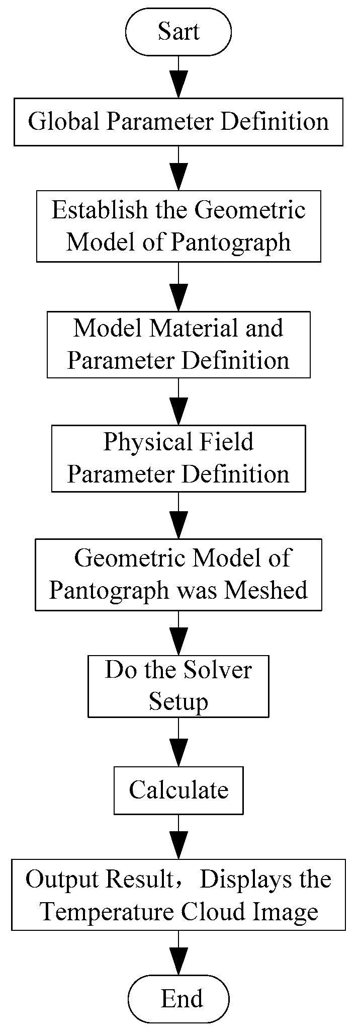
2.1. Simulation Solving Process of Pantograph Arc

The temperature field of the pantograph–catenary arc is simulated and modeled based on COMSOL software, and the specific modeling solution process is shown in Figure 1.

2.2. Hypothesis of Related Properties of Pantograph Arc

The physical and chemical changes in the urban rail pantograph–catenary arc are very complex. In order to approximate the actual situation as much as possible in the simulation modeling process, facilitate the analysis of the temperature characteristics of the arc, and simplify the calculation degree, the following assumptions are proposed for the finite element model of the pantograph–catenary arc.

• Only static pantograph–catenary arc is considered, that is, stable arc already exists in the solution process.
• The material characteristics of the pantograph–catenary system change little with temperature, which is ignored when solving.
• The air solution domain in the simulation model is the ideal air domain.
• The static pantograph arc in the model meets the requirements of local thermodynamic equilibrium.

2.3. Establishment of Geometric Model of Pantograph

The solution of the two-dimensional geometric model by COMSOL software is actually the result obtained by stretching the two-dimensional model into a three-dimensional model and then calculating.

Therefore, for the static pantograph–catenary arc, a two-dimensional geometric simplified model is adopted for simulation of the pantograph–catenary system. The arc geometry model of pantograph and catenary is established along the contact line section, as shown in Figure 2.

In Figure 2, the size parameter of the contact line is set according to the contact line of the pantograph–catenary system of the actual urban rail train. The radius is 6.5 mm. The two grooves in the contact line are used by the wire clamp to fix the contact wire.

In the simulation model of the pantograph–catenary arc, due to the non-smooth contact line and other factors, the pantograph will produce arc offline. It is assumed that the maximum pantograph jitter range is 1 mm, and the maximum pantograph jitter gap is used for simulation experiment.

The contact wire material is set as pure copper wire, and the pantograph slide plate material is set as pure carbon slide plate. The geometric size of the carbon slide plate is 220 $\times$22 mm. The specific parameters of the pantograph and catenary are shown in

Table 1. Contact line with carbon slide parameters.

Material	Density(Kg/m3)	Specific Heat /(J/(kg·K))	Coefficient of Thermal Conductivity /(W/(m·K))
Contact wire	8960	385	400
Carbon skateboard	2400	710	151

.

2.4. Heat Transfer Module Theory and Equations

In this paper, based on the heat transfer theory, the pantograph–catenary arc simulation model was established. By coupling the arc-related physical field, the equations were established and solved, and finally, the distribution of the arc temperature field was obtained. Set the arc duration, analyze the arc temperature distribution, and get the relationship between the arc duration and the arc temperature. The COMSOL simulation software solver is set as transient in the model, which is convenient to observe the instantaneous static arc temperature change.

During the establishment of this model, mass conservation equation, momentum conservation equation, and energy conservation equation were followed [21,22].

• Mass conservation equation

Mass can neither appear nor disappear, and in any physical system isolated from its surroundings, its total mass will remain the same regardless of any change or process. Take a micro hexahedron arbitrarily in the fluid and assume that the fluid velocity of the hexahedron in the x, y, and z axes is u, v, and w, respectively. Mass change per unit time in the direction of x, y and z axes:

$$\left\{\begin{array}{l}[\rho u+\frac{\partial (\rho u)}{\partial x}\Delta x]\Delta y\Delta z-\rho u\Delta y\Delta z=\frac{\partial (\rho u)}{\partial x}\Delta x\Delta y\Delta z\\ [\rho v+\frac{\partial (\rho v)}{\partial y}\Delta y]\Delta x\Delta z-\rho v\Delta x\Delta z=\frac{\partial (\rho v)}{\partial y}\Delta x\Delta y\Delta z\\ [\rho w+\frac{\partial (\rho w)}{\partial z}\Delta z]\Delta x\Delta y-\rho w\Delta x\Delta y=\frac{\partial (\rho w)}{\partial z}\Delta x\Delta y\Delta z\end{array}\right.$$

(1)

The change in mass per unit volume per unit time is as follows:

$$\frac{\partial \rho }{\partial t}\Delta x\Delta y\Delta z$$

(2)

The mass conservation equation can be derived as follows:

$$\frac{\partial (\rho u)}{\partial x}\Delta x\Delta y\Delta z+\frac{\partial (\rho v)}{\partial y}\Delta x\Delta y\Delta z+\frac{\partial (\rho w)}{\partial z}\Delta x\Delta y\Delta z+\frac{\partial \rho }{\partial t}\Delta x\Delta y\Delta z=0$$

(3)

To sort out:

$$\frac{\partial \rho }{\partial t}+\frac{\partial (\rho u)}{\partial x}+\frac{\partial (\rho v)}{\partial y}+\frac{\partial (\rho w)}{\partial z}=0$$

(4)

The Navier–Stokes mass conservation equation is obtained as follows:

$$\frac{\partial \rho }{\partial t}+\nabla (\rho \cdot u)=0$$

(5)

where $\rho$ is the fluid density and u is the fluid velocity.

2.

Momentum conservation equation

According to Newton’s second law, change of momentum in unit time + outgoing momentum in unit time – incoming momentum in unit time = internal force + external force. Take a micro hexahedron randomly in the fluid and assume that the fluid velocity in the three directions of the hexahedron is u, v, and w on the x, y, and z axes, respectively. Then, the change of unit time momentum in the x, y, and z axes is shown in the equation below:

$$\left\{\begin{array}{l}[\rho u^{2}w+\frac{\partial (\rho u^{2}w)}{\partial x}\Delta x]\Delta y\Delta z-\rho u^{2}w\Delta y\Delta z=\frac{\partial (\rho u^{2}w)}{\partial x}\Delta x\Delta y\Delta z\\ [\rho uvw+\frac{\partial (\rho uvw)}{\partial y}\Delta y]\Delta x\Delta z-\rho uvw\Delta x\Delta z=\frac{\partial (\rho uvw)}{\partial y}\Delta x\Delta y\Delta z\\ [\rho u{w}^2+\frac{\partial (\rho u{w}^2)}{\partial z}\Delta z]\Delta x\Delta y-\rho u{w}^2\Delta x\Delta y=\frac{\partial (\rho u{w}^2)}{\partial z}\Delta x\Delta y\Delta z\end{array}\right.$$

(6)

The change of flow momentum per unit time per unit volume is as follows:

$$\frac{\partial (\rho u)}{\partial t}\Delta x\Delta y\Delta z$$

(7)

The variation of force per unit time on the x, y, and z axes is shown in the equation below:

$$\left\{\begin{array}{l}-\frac{\partial ({\sigma }_x)}{\partial x}\Delta x\Delta y\Delta z+\frac{\partial ({\tau }_{xy})}{\partial y}\Delta x\Delta y\Delta z+\frac{\partial ({\tau }_{xz})}{\partial z}\Delta x\Delta y\Delta z+X\Delta x\Delta y\Delta z\\ -\frac{\partial ({\sigma }_y)}{\partial y}\Delta x\Delta y\Delta z+\frac{\partial ({\tau }_{yx})}{\partial x}\Delta x\Delta y\Delta z+\frac{\partial ({\tau }_{yz})}{\partial z}\Delta x\Delta y\Delta z+Y\Delta x\Delta y\Delta z\\ -\frac{\partial ({\sigma }_z)}{\partial z}\Delta x\Delta y\Delta z+\frac{\partial ({\tau }_{zx})}{\partial x}\Delta x\Delta y\Delta z+\frac{\partial ({\tau }_{zy})}{\partial y}\Delta x\Delta y\Delta z+Z\Delta x\Delta y\Delta z\end{array}\right.$$

(8)

The momentum conservation equation can be written as the equation below:

$$\left\{\begin{array}{l}\rho \frac{\partial u}{\partial t}+u\frac{\partial u}{\partial x}+v\frac{\partial u}{\partial y}+w\frac{\partial u}{\partial z}=-\frac{\partial ({\sigma }_x)}{\partial x}+\frac{\partial ({\tau }_{xy})}{\partial y}+\frac{\partial ({\tau }_{xz})}{\partial z}+X\\ \rho \frac{\partial u}{\partial t}+u\frac{\partial v}{\partial x}+v\frac{\partial v}{\partial y}+w\frac{\partial v}{\partial z}=-\frac{\partial ({\sigma }_y)}{\partial y}+\frac{\partial ({\tau }_{yx})}{\partial x}+\frac{\partial ({\tau }_{yz})}{\partial z}+Y\\ \rho \frac{\partial u}{\partial t}+u\frac{\partial w}{\partial x}+v\frac{\partial w}{\partial y}+w\frac{\partial w}{\partial z}=-\frac{\partial ({\sigma }_z)}{\partial z}+\frac{\partial ({\tau }_{zx})}{\partial x}+\frac{\partial ({\tau }_{zy})}{\partial y}+Z\end{array}\right.$$

(9)

Navier–Stokes momentum conservation equation can be obtained by transformation as follows:

$$\rho \frac{\partial u}{\partial t}+\rho (u\cdot \nabla )u=\nabla \cdot [-pI+\tau ]+F$$

(10)

where $\rho$ is the fluid density, u is the fluid velocity, p is the pressure, I is the impulse, $\tau$ is the viscous stress, and F is the volume force.

3.

Energy conservation equation

Conservation of energy is the first law of thermodynamics. It means that in a closed, isolated system, the total energy remains the same. System energy change per unit time = fluid transfer energy + heat transfer energy + internal heat source energy − net work coming out of the fluid. Take a micro hexahedron in the fluid and assume that the fluid velocity in the three directions of the hexahedron is u, v, and w on the x, y, and z axes, respectively. Then, the change of fluid transfer energy per unit time in the x, y, and z axes is shown in the equation below:

$$\left\{\begin{array}{l}[\rho ue+\frac{\partial (\rho ue)}{\partial x}\Delta x]\Delta y\Delta z-\rho ue\Delta y\Delta z=\frac{\partial (\rho ue)}{\partial x}\Delta x\Delta y\Delta z\\ [\rho ve+\frac{\partial (\rho ve)}{\partial y}\Delta y]\Delta x\Delta z-\rho ve\Delta x\Delta z=\frac{\partial (\rho ve)}{\partial y}\Delta x\Delta y\Delta z\\ [\rho we+\frac{\partial (\rho we)}{\partial z}\Delta z]\Delta x\Delta y-\rho we\Delta x\Delta y=\frac{\partial (\rho we)}{\partial z}\Delta x\Delta y\Delta z\end{array}\right.$$

(11)

The variation of heat transfer energy per unit time in the x, y, and z axes is as follows:

$$\left\{\begin{array}{l}[q_x^{″}+\frac{\partial q_x^{″}}{\partial x}\Delta x]\Delta y\Delta z-q_x^{″}\Delta y\Delta z=\frac{\partial q_x^{″}}{\partial x}\Delta x\Delta y\Delta z\\ [q_y^{″}+\frac{\partial q_y^{″}}{\partial y}\Delta y]\Delta x\Delta z-q_y^{″}\Delta x\Delta z=\frac{\partial q_y^{″}}{\partial y}\Delta x\Delta y\Delta z\\ [q_z^{″}+\frac{\partial q_z^{″}}{\partial z}\Delta z]\Delta x\Delta y-q_z^{″}\Delta x\Delta y=\frac{\partial q_z^{″}}{\partial z}\Delta x\Delta y\Delta z\end{array}\right.$$

(12)

The variation of heat source energy per unit time is as follows:

$$q^{″\prime }\Delta x\Delta y\Delta z$$

(13)

The change in net efferent work per unit time in a fluid is as follows:

$$\left\{\begin{array}{l}-[{\sigma }_x\frac{\partial u}{\partial x}-{\tau }_{xy}\frac{\partial u}{\partial y}-{\tau }_{xz}\frac{\partial u}{\partial z}+{\sigma }_y\frac{\partial v}{\partial y}-{\tau }_{yx}\frac{\partial v}{\partial x}-{\tau }_{yz}\frac{\partial v}{\partial z}+{\sigma }_z\frac{\partial w}{\partial z}-{\tau }_{zx}\frac{\partial w}{\partial x}-{\tau }_{zy}\frac{\partial w}{\partial y}]\Delta x\Delta y\Delta z\\ -[u\frac{\partial {\sigma }_x}{\partial x}-u\frac{\partial {\tau }_{xy}}{\partial y}-u\frac{\partial {\tau }_{xz}}{\partial z}+v\frac{\partial {\sigma }_y}{\partial y}-v\frac{\partial {\tau }_{yx}}{\partial x}-v\frac{\partial {\tau }_{yz}}{\partial z}+w\frac{\partial {\sigma }_z}{\partial z}-w\frac{\partial {\tau }_{zx}}{\partial x}-w\frac{\partial {\tau }_{zy}}{\partial y}]\Delta x\Delta y\Delta z\end{array}\right.$$

(14)

The change in system energy per unit volume per unit time is as follows:

$$\frac{\partial (\rho e)}{\partial t}\Delta x\Delta y\Delta z$$

(15)

The energy conservation equation can be obtained as:

$$\left\{\begin{array}{l}\frac{\partial (\rho e)}{\partial t}\Delta x\Delta y\Delta z=-[\frac{\partial (\rho ue)}{\partial x}+\frac{\partial (\rho ve)}{\partial y}+\frac{\partial (\rho we)}{\partial z}]\Delta x\Delta y\Delta z-[\frac{\partial q_x^{″}}{\partial x}+\frac{\partial q_y^{″}}{\partial y}+\frac{\partial q_z^{″}}{\partial z}]\Delta x\Delta y\Delta z+\\ q^{″\prime }\Delta x\Delta y\Delta z-[{\sigma }_x\frac{\partial u}{\partial x}-{\tau }_{xy}\frac{\partial u}{\partial y}-{\tau }_{xz}\frac{\partial u}{\partial z}+{\sigma }_y\frac{\partial v}{\partial y}-{\tau }_{yx}\frac{\partial v}{\partial x}-{\tau }_{yz}\frac{\partial v}{\partial z}+{\sigma }_z\frac{\partial w}{\partial z}-{\tau }_{zx}\frac{\partial w}{\partial x}-{\tau }_{zy}\frac{\partial w}{\partial y}]\Delta x\Delta y\Delta z-\\ [u\frac{\partial {\sigma }_x}{\partial x}-u\frac{\partial {\tau }_{xy}}{\partial y}-u\frac{\partial {\tau }_{xz}}{\partial z}+v\frac{\partial {\sigma }_y}{\partial y}-v\frac{\partial {\tau }_{yx}}{\partial x}-v\frac{\partial {\tau }_{yz}}{\partial z}+w\frac{\partial {\sigma }_z}{\partial z}-w\frac{\partial {\tau }_{zx}}{\partial x}-w\frac{\partial {\tau }_{zy}}{\partial y}]\Delta x\Delta y\Delta z\end{array}\right.$$

(16)

The Navier–Stokes energy conservation equation is obtained by transformation:

$$\rho C_p\frac{\partial T}{\partial t}+\rho C_{p}u\cdot \nabla T=\nabla \cdot (k\nabla T)+Q+\tau :S+\frac{T}{\rho }{(\frac{\partial \rho }{T})}_p(\frac{\partial p_a}{\partial t}+u\cdot \nabla p_a)$$

(17)

where $\rho$ is the fluid density, $C_p$ is the specific heat capacity of the fluid at room temperature and pressure, $u$ is the fluid velocity, T is the temperature, k is the thermal coefficient, $\tau$ is the viscous stress, S is the surface area, Q is the heat source term, and $p_a$ is the fluid pressure.

2.5. Setting of Initial and Boundary Conditions

In order to obtain the temperature nephogram distribution of the pantograph–catenary arc, it is necessary to set the boundary of the arc model. The initial temperature condition was set to 300 K, the thickness of the air solution domain was set to 50 mm, and the absolute fluid pressure was set to 1 atm. For the surface of the pantograph–catenary system, air convection heat transfer boundary conditions are set up because in the process of the locomotive running faster, air flow speed is relatively fast; so, this cannot be ignored when calculating. Choose the way to forced convection in the simulation software, the convective heat transfer coefficient setting [23] of 100 W/m²·(K), and define the arc heat flux boundary condition for the 10¹⁰ W/m². In order to explore the relationship between the arc duration and arc temperature, the arc duration was set as 0.1 s, 0.4 s, 0.7 s, and 1 s, respectively.

3. Analysis of Simulation Results

The high temperature characteristic of the pantograph–catenary arc will cause ablative effect on the surface material of the arc system, which may cause damage to the components of the pantograph–catenary system and affect the flow of the locomotive [24]. Therefore, it is necessary to study the temperature distribution of the arc in the field and the relationship between the arc temperature and duration. The arc model of the static arc was established in COMSOL finite element software to simulate the temperature distribution of the static arc in different duration and different gap of the arc, and then the relationship between the arc duration and the arc temperature was analyzed.

1.

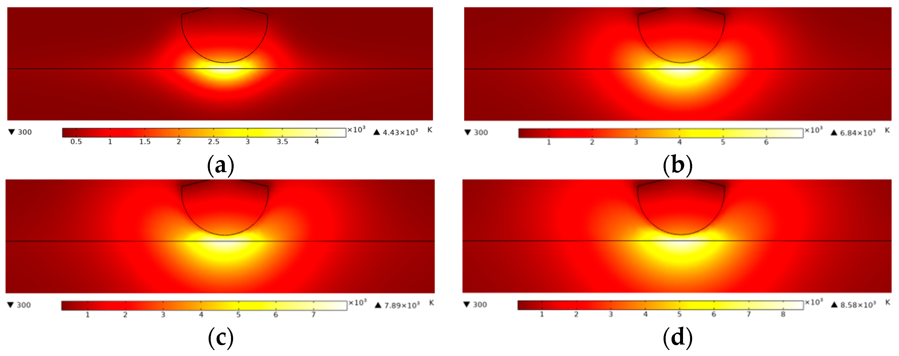
In the anti-seismic software, adjust the gap between the pantograph and contact line to 1 mm and obtain the temperature distribution cloud diagram of the pantograph–catenary arc when t = 0.1 s, 0.4 s, 0.7 s, and 1 s, as shown in Figure 3.

In the simulation software, when the gap between the pantograph and contact line is set to 1 mm, the two-dimensional transvestite is defined and the two-dimensional transvestite is the upper half-axis of the arc central axis. The simulation software is used to extract the temperature curves of 10 times within 0~1 s of the arc duration, as shown in Figure 4.

As can be seen from the temperature distribution cloud diagram of the pantograph–catenary arc, when the gap of the arc grid is fixed at 1 mm, the arc plasma coverage area becomes larger and the arc temperature increases with the increase in arc duration, and the temperature in the central area of the arc is the highest, which can reach more than 8000 K.

As can be seen from the temperature curve of the axis, as the temperature of the arc center gradually decreases from the periphery, the temperature changes the fastest between 4 mm and 12 mm.

2.

When the gap is fixed at 2 mm, the temperature change of the arc duration is observed at 0.1 s, 0.4 s, 0.7 s, and 1 s. The temperature distribution cloud diagram of the pantograph arc is shown in Figure 5.

When the gap of the pantograph–catenary is 2 mm, the two-dimensional transvestite is defined in the simulation software, and the two-dimensional transvestite is defined as the upper half-axis of the arc central axis. The simulation software is used to extract the temperature curves for 10 durations within 0~1 s, as shown in Figure 6.

As can be seen from the temperature distribution cloud diagram in Figure 6, when the gap is constant at 2 mm, the arc coverage area becomes larger, and the arc temperature increases with the increase in the arc duration. The temperature of the arc center is the highest, reaching above 8000 K. As can be seen from the temperature curve of the axis, as the temperature of the arc center decreases gradually from the periphery, the temperature changes the fastest between 4 mm and 12 mm, but the maximum temperature decreases somewhat compared with the 1 mm gap of the pantograph–catenary arc.

3.

When the gap of the pantograph–catenary is 3 mm, the arc temperature changes when the arc duration is 0.1 s, 0.4 s, 0.7 s, and 1 s, and the temperature distribution cloud diagram is shown in Figure 7.

When the gap of the pantograph–catenary is 3 mm, two-dimensional trans sects are defined in the simulation software, which is defined as the upper half-axis of the arc central axis. The temperature curves of 10 durations within 0~1 s are extracted by the simulation software, as shown in Figure 8.

As can be seen from the temperature distribution cloud diagram of the pantograph–catenary arc, when the gap of the arch grid is 3 mm constant, the arc coverage area becomes larger and the arc temperature rises with the increase in arc duration, and the temperature in the central area reaches above 7000 K. As can be seen from the temperature curve, as the temperature of the arc center decreases gradually from the periphery, the temperature changes the fastest between 4 mm and 12 mm, but the maximum temperature decreases somewhat compared with that between 1 mm and 2 mm of the pantograph–catenary gap.

In order to more intuitively observe the relationship between the arc duration and arc temperature, the changes of the arc center temperature over time under the three conditions of arc clearance of 1 mm, 2 mm, and 3 mm are listed in,

Table 2. Simulation data of arc center temperature when pantograph gap is 1 mm.

Time(s)	0.1	0.2	0.3	0.4	0.5	0.6	0.7	0.8	0.9	1
Temperature(K)	4430	5570	6310	6840	7250	7590	7890	8140	8370	8580

,

Table 3. Simulation data of arc center temperature when pantograph gap is 2 mm.

Time(s)	0.1	0.2	0.3	0.4	0.5	0.6	0.7	0.8	0.9	1
Temperature(K)	3950	5030	5760	6330	6760	7100	7400	7650	7870	8080

and

Table 4. Simulation data of arc center temperature when pantograph gap is 3 mm.

Time(s)	0.1	0.2	0.3	0.4	0.5	0.6	0.7	0.8	0.9	1
Temperature(K)	3720	4750	5430	5950	6370	6710	7020	7290	7530	7740

, respectively.

It can be seen from the data in the table that under the condition of a certain gap of the pantograph–catenary system, the arc temperature increases with the increase in the duration. Under the condition of constant duration, the arc temperature decreases with the increase in the gap.

4. Experimental Verification of Arc Simulation Model

In order to verify the reliability of the arc simulation model, the temperature characteristics of the pantograph–catenary arc are studied by using the self-made pantograph–catenary electrical contact experimental device in the laboratory. The experimental device materials and various parameter settings are consistent with the simulation model. The schematic diagram of the pantograph–catenary arc experimental device is shown in Figure 9. Through the rotation of the wheel and the servo motor to control the carbon slide up and down, horizontal movement, simulate the locomotive in the operation of the pantograph–catenary system.

The test device shown in the figure uses single-phase DC power supply. R and L are used to simulate the load impedance of the locomotive. Current transformers and voltage transformers are used to collect the current and voltage values of the locomotive during operation. Because the arc temperature is very high, the spectrometer is used to collect the arc emission spectrum to calculate the arc burning temperature, and the experimental data of current, voltage, and arc temperature are obtained by industrial computer.

In the simulation model, it is assumed that the maximum range of pantograph jitter of the locomotive in operation is 1 mm, 2 mm, and 3 mm. Therefore, the gap between pantograph and catenary in the experimental device is also set as 1 mm, 2 mm, and 3 mm to compare with the simulation data. The change of experimental arc center temperature over time was recorded. According to the experimental data, the computer graphics software was used to draw the comparison curve graph between simulation and experiment, as shown in Figure 10.

In Figure 10, the simulation results and test results of arc temperature in different gaps show that when the gap is fixed, the arc temperature increases with the increase in duration. The temperature rises obviously with time between 0 s and 0.4 s, and changes slowly after 0.6 s. When the arc duration is fixed, the arc temperature decreases with the increase in the gap.

The data comparison results show that the trend of the experimental curve is roughly the same as that of the simulation curve, but there are slight fluctuations. This is because the infinite setting of the air solution domain cannot be realized in the simulation process, the change of the material characteristics of the pantograph–catenary system with the temperature is ignored, and the influence of the joule heat generated in the contact line and pantograph on the arc temperature is not considered. In general, it can be concluded from both experimental and simulation data that the arc temperature increases with the increase in arc duration. Therefore, the pantograph–catenary arc simulation model established in this paper can reflect the actual pantograph arc temperature of urban rail.

5. Conclusions

The arc of urban rail will cause different degrees of ablative effect on the pantograph slide and contact line. Because the arc of urban rail is accidental and the duration is short, it is difficult to realize the on-board temperature detection. In order to investigate the temperature distribution of arc in urban rail, the finite element software is used to establish a simulation model of the pantograph–catenary arc in urban rail. The arc temperature field of the arc was solved by the model, and the cloud diagram of the arc temperature distribution, the temperature curve of the upper half-axis of the arc central axis, and the correlation data of the arc central temperature and the arc duration were output. Then, the relationship between arc temperature and arc duration is studied. In order to verify that the established model can correctly reflect the temperature variation of the pantograph–catenary arc, the temperature detection experiment of the pantograph–catenary arc in the laboratory is carried out, and the conclusions are as follows:

• The pantograph jigs on board, resulting in the offline of the pantograph–catenary system. When the gap between the pantograph and contact line is fixed at 1 mm, 2 mm, and 3 mm, within 1 s, with the increase in the arc duration, the arc coverage area increases, and the arc temperature also rises gradually. In the range of the experimental gap, when the arc duration is constant, the larger the gap, the smaller the arc temperature.
• The coverage area of the pantograph–catenary arc image obtained by the simulation model is generally elliptical. The temperature of the arc center area is the highest, which can reach more than 8000 K. The temperature of any point in the arc coverage area gradually decreases with the increase in the distance from the center point, and the temperature of the edge area is the lowest.
• The experimental arc temperature data and the arc temperature data obtained from the simulation model vary with the gap and duration of the arc, which verifies the feasibility of the simulation model established in this paper for the pantograph–catenary arc temperature analysis. However, due to the inability to realize the infinite air solution domain in the simulation model, the failure to consider the material characteristics of the pantograph–catenary system changing with temperature, and the neglect of the contact line and the joule heat generated in the pantograph on the arc impact, there are differences between the laboratory arc experimental data and the simulation data. Therefore, there is room for further improvement of this pantograph arc model.

References

- Yu, X. Development and Application of Urban Rail Transit Arc Detection System Based on Solar Blind Zone. Ph.D. Thesis, Lanzhou Jiaotong University, Lanzhou, China, 2021. [Google Scholar]
- Li, X.; Zhu, F.; Qiu, R.; Tang, Y. Research on the influence of metro arc on airport instrument landing system. J. China Railw. Soc. 2018, 40, 97–102. [Google Scholar]
- Song, Y.; Wang, Z.; Liu, Z.; Wang, R. A spatial coupling model to study dynamic performance of pantograph-catenary with vehicle-track excitation. Mech. Syst. Signal Process. 2021, 151, 107336. [Google Scholar] [CrossRef]
- Wei, X.K.; Meng, H.F.; He, J.H.; Jia, L.M.; Li, Z.G. Wear analysis and prediction of rigid catenary contact wire and pantograph strip for railway system. Wear 2020, 442–443, 203118. [Google Scholar] [CrossRef]
- Shi, H.; Chen, G.; Yang, Y. A comparative study on pantograph-catenary models and effect of parameters on pantograph-catenary dynamics under crosswind. J. Wind. Eng. Ind. Aerodyn. 2021, 211, 104587. [Google Scholar] [CrossRef]
- Zhang, Y.; Li, C.; Pang, X.; Song, C.; Ni, F.; Zhang, Y. Evolution processes of the tribological properties in pantograph/catenary system affected by dynamic contact force during current-carrying sliding. Wear 2021, 477, 203809. [Google Scholar] [CrossRef]
- Xu, M. Development of Experimental Platform and Research on Characteristics of Pantograph Arc. Master’s Thesis, Beijing Jiaotong University, Beijing, China, 2020. [Google Scholar]
- Huanga, S.; Zhai, Y.; Zhang, M.; Hou, X. Arc detection and recognition in pantograph–catenary system based on convolutional neural network. Inf. Sci. 2019, 501, 363–376. [Google Scholar] [CrossRef]
- Signorino, D.; Giordano, D.; Mariscotti, A.; Gallo, D.; Femine, A.D.; Balic, F.; Quintana, J.; Donadio, L.; Biancucci, A. Dataset of measured and commented pantograph electric arcs in DC railways. Data Brief 2020, 31, 105978. [Google Scholar] [CrossRef] [PubMed]
- Song, Y.; Wang, H.; Liu, Z. An investigation on the current collection quality of railway pantograph-catenary systems with contact wire wear degradations. IEEE Trans. Instrum. Meas. 2021, 70, 9003311. [Google Scholar] [CrossRef]
- Yang, H.; Hu, B.; Liu, Y.; Cui, X.; Jiang, G. Influence of reciprocating distance on the delamination wear of the carbon strip in pantograph–catenary system at high sliding-speed with strong electrical current. Eng. Fail. Anal. 2019, 104, 887–897. [Google Scholar] [CrossRef]
- Yu, X.; Su, H. Pantograph arc detection of urban rail based on photoelectric conversion mechanism. IEEE Access 2020, 8, 14489–14499. [Google Scholar] [CrossRef]
- Fan, F.; Wank, A.; Seferi, Y.; Stewart, B.G. Pantograph arc location estimation using resonant frequencies in DC railway power systems. IEEE Trans. Transp. Electrif. 2021, 7, 3083–3095. [Google Scholar] [CrossRef]
- Hao, J.; Gao, G.; Xu, P.; Wei, W.; Hu, Y.; Wu, G. Model of and electrode coupling in pantograph arc considering electrode melting. High Volt. Technol. 2018, 44, 1668–1676. [Google Scholar]
- Yu, X.; Su, H. Detection system of urban rail pantograph arc based on primary integral value of PMT voltage. J. China Railw. Soc. 2019, 41, 51–58. [Google Scholar]
- Yang, Z.; Xu, P.; Wei, W.; Gao, G.; Zhou, N.; Wu, G. Influence of the crosswind on the pantograph arcing dynamics. IEEE Trans. Plasma Sci. 2020, 48, 2822–2830. [Google Scholar] [CrossRef]
- Hao, J.; Gao, G. Dynamic characteristics of plasma in pantograph arc during pantograph lowering. J. China Railw. Soc. 2018, 40, 65–70. [Google Scholar]
- Hu, Y.; Gao, G.; Chen, X.; Zhang, T.; Wei, W.; Wu, G. Research on pantograph arc in pantograph lowering process based on spectrum. High Volt. Technol. 2018, 44, 3980–3986. [Google Scholar]
- Wang, J. Research on the key characteristics of DC pantograph arc. Master’s Thesis, Liaoning Technical University, Fuxin, China, 2021. [Google Scholar]
- Lei, D.; Zhang, T.; Duan, X.; Gao, G.; Wei, W.; Wu, G. Influence of train running speed on electric characteristics of pantograph arc. J. China Railw. Soc. 2019, 41, 50–56. [Google Scholar]
- Zhu, G.; Wu, G.; Han, W.; Gao, G.; Liu, X. Simulation and analysis on steady state characteristics of pantograph arc during static lifting and lifting of high-speed train. J. China Railw. Soc. 2016, 38, 42–47. [Google Scholar]
- Xu, Z.; Gao, G.; Wei, W.; Yang, Z.; Xie, W.; Dong, K.; Ma, Y.; Yang, Y.; Wu, G. Characteristics of pantograph-catenary arc under low air pressure and strong airflow. High Volt. 2022, 7, 369–381. [Google Scholar] [CrossRef]
- Li, T. Analysis of Electric Characteristics and Temperature Field of Pantograph arc. Master’s Thesis, Beijing Jiaotong University, Beijing, China, 2019. [Google Scholar]
- Li, B.; Luo, C.; Wang, Z. Application of GWO-SVM algorithm in arc detection of pantograph. IEEE Access 2020, 8, 173865–173873. [Google Scholar] [CrossRef]