Coordinated Lateral Stability Control of Autonomous Vehicles Based on State Estimation and Path Tracking

Abstract

This paper proposes a coordinated control system of autonomous vehicles’ lateral stability based on state estimation and path tracking, which contributes to enhancing path-tracking capability and at the same time maintaining the stability of autonomous vehicles driving in complex and dynamic road conditions. First, an extended Kalman filter observer is designed to estimate the vehicle parameters. Then, based on the single-point preview theory, an adaptive preview time model is built for the accuracy of path tracking. When designing the direct yaw-moment controller, sideslip angle and yaw rate, two critical parameters for lateral dynamic stability control are considered, and the single-wheel braking method is utilized to reasonably distribute the additional yaw moment to a certain wheel. To make full use of active front steering and direct yaw-moment control, the critical steering angle of the front wheel is determined, and a switching function is formulated. Co-simulation shows that the suggested coordinated control system can effectively strengthen maneuvering stability and simultaneously satisfy tracking accuracy.

1. Introduction

Along with the worldwide use of autonomous vehicles and the technological advance of vehicle electronics, how to improve path-tracking ability and simultaneously maintain the driving stability of autonomous vehicles has become a practical challenge for many automotive manufacturers and researchers. Up to now, a variety of stability control systems have been developed and successfully commercialized, for instance, the anti-lock braking system (ABS), vehicle stability assist (VSA), electronic stability program (ESP) and so on, all of which have significantly improved the safety of vehicles.

In order to better investigate the lateral stability performance of autonomous vehicles, it is necessary to accurately obtain the motion parameters of the vehicle during the driving process, which include yaw rate, sideslip angle, longitudinal velocity, etc. A variety of state observers have been developed for parameter identification. Kanghyun Nam et al. [1] designed a state observer derived from extended Kalman filtering (EKF) theory to estimate the sideslip angle, which contributes to improving the vehicle stability of in-wheel-motor-driven electric vehicles (IWM-EVs). Zhou Bing et al. [2] designed an EKF algorithm to solve the problem of steering wheel torque change in the integrated system of electric power steering (EPS) and active front steering (AFS), according to which the abrupt change of steering wheel torque was used and the combination of vehicle state estimation and vehicle control was realized. Peng Hang et al. [3] designed a state observer using an unscented Kalman filter (UKF) to measure lateral velocity when considering an integrated chassis control algorithm for path tracking utilizing four-wheel steering (4WS) and direct yaw-moment control (DYC). Currently, longitudinal velocity and yaw rate can be easily measured by sensors, while sideslip angle, a significant reference indicator of lateral stability, is still hard to measure directly with sensors [4,5]. Considering its high calculation accuracy, strong filtering stability, and easier engineering implementation [6], an extended Kalman filter state observer has been chosen for the estimation of sideslip angle.

To achieve a stable status, accurate tracking of complex trajectories is one of the most significant points. So-called path-tracking control [7,8] refers to the final step in the realization of autonomous driving after information sensing, information fusion and path planning of the surrounding environment, the core problem of which is how to achieve automatic steering and straight driving. Its goal is to make the vehicle drive along the pre-determined reference trajectory, which means assisting the vehicle in tracking the reference trajectory as much as possible through certain control methods and ensuring the maneuvering stability of the driver and passengers at the same time when driving. To track the reference trajectory and improve tracking accuracy, many researchers at home and abroad have conducted in-depth research via a variety of path-tracking methods of autonomous vehicles, which includes PID control [9], fuzzy control [10], model predictive control (MPC) [11], sliding mode control (SMC) [12] and multi-control [13,14,15]. A combination of path tracking and lane detection can also play a critical role in the autonomous control of intelligent electric vehicles [16].

However, in the above studies, the preview time, an important parameter for trajectory tracking, is often set to a fixed value, which may decrease the accuracy of autonomous vehicles driving under dynamic and complex conditions. To improve the vehicle trajectory following capability and driving stability, considering the actual complex driving conditions, this paper designs an adaptive preview time controller.

In terms of a vehicle′s driving conditions, lateral instability can easily occur while steering, the moment when the likelihood of a traffic accident is greatly increased. Under extreme operating conditions, both active front steering (AFS) and direct yaw-moment control (DYC) can contribute to maintaining lateral stability. The AFS system, without affecting the driver′s operation, adjusts the lateral force of the vehicle through small angle changes of the front wheels, so as to control the vehicle in the yaw direction to improve the driving safety performance [17,18]. The DYC system, enabling the vehicle to ensure tire adhesion is maintained in a linear range, will generate an additional yaw moment which will be distributed to each wheel independently through applying braking or driving force and improve the stability of vehicle movement [19,20].

However, both AFS and DYC alone have their limitations, leading to their control effect not being obvious. The AFS system will not affect the driving performance of the vehicle, but it only works in the linear area of the tires, while the DYC system can work in the nonlinear area, but its intervention will significantly reduce the longitudinal velocity and affect the driver′s handling experience and comfort. To verify the stability of autonomous vehicles during path tracking, while at the same time ensuring that vehicles adapt to complex driving conditions and make full use of AFS and DYC, many researchers have used various control methods to study coordinated control, which has dramatically advanced the development of vehicles’ stability control systems.

In the selection of vehicle reference models, a two-degree-of-freedom (2-DOF) vehicle model is typically applied by researchers to derive two critical parameters for lateral dynamic stability control, which are the referred yaw rate and the sideslip angle. When considering the status of each wheel and the yaw movement, a vehicle model with more freedom is commonly utilized instead, which can provide researchers with more accurate vehicle parameter data, including yaw rate, vertical load, sideslip angle and so on. Examples include 7-DOF vehicle models [21], 8-DOF vehicle models [22,23], and 14-DOF vehicle models [24]. In terms of integrated control methods, researchers have also tried many of them, one of which is the model predictive control (MPC) method. Ji Yan et al. [25] introduced an AFS and DYC integrated controller based on MPC and established a bicycle model formula which can help detect the reasonable front wheel steering angle as well as additional yaw moment. Taehyun shim et al. [26] suggested an autonomous vehicle crash protection system including motion planners, active vehicle steering control and active wheel torque distribution, applying the method of MPC, where motion planners determined impact-free trajectories based on multiple parameterization and control systems based on MPC focused on calculating the steering angle and torque for each wheel for the purpose of reliably maintaining a collision-free reference path. Researchers also used fuzzy control method; Sun Tao et al. [22] described a controller that integrated DYC with AFS for lateral speed estimation, which used fuzzy control algorithms to obtain additional direct yaw moment and then analyzed the required front wheel steering angles. There are also researchers who have suggested ways to use feed-forward feedback control; A. Goodarzi et al. [27] presented a new optimal control system for lateral trajectory tracking of automated vehicles coordinated by active steering control (ASC) and DYC, where the road curvature and the lateral offset were set as the feedback/feed forward signals and the control targets chose the generated steering angle and additional yaw moment signals. There is no doubt that slide mode control (SMC) would also be considered by different researchers; Li, Bin et al. [28], for example, proposed a vehicle stability control solution that integrated DYC and AFS, in which the upper controller of the system applied the SMC method to calculate the desired yaw moment and rear wheel steering angle; other examples include Zhang Jiaxu et al. [29], who proposed an integrated vehicle chassis control (IVCC) strategy that coordinated AFS and DYC through hierarchical control, where the fast terminal sliding mode control (FTSMC) was applied in the upper controller of the system to generate corresponding yaw moment, and then in the design of lower one, the results were transformed into the desired longitudinal slips and front wheel steering angle increment using the zero-space-based control redistribution theory and inverse tire model; Choker, Abba et al. [30] developed a global chassis controller coordinating AFS, DYC and active suspension control in accordance with the super-twisting sliding mode theory. Meanwhile, by applying fuzzy logic rules and considering stability standards, a decision-layer was also designed. Universally used by researchers, neural network theory has also been utilized when considering coordinating AFS with DYC. For example, Yao Xinxin et al. [31] proposed a coordinated controller utilizing stability judgment by applying self-organizing feature map (SOFM) neural networks and K-means algorithms. Through weighting the coordinated system based on vehicle stability levels, a controller was proposed that achieved both track accuracy and handling stability. Of course, there are some other researchers who have adopted other research methods. For example, by applying direct Lyapunov methods, Ding Nenggen et al. [23] established a non-linear 8-DOF vehicle model applying the adaptive integrated control algorithm in accordance with DYC and AFS.

According to the above analysis, most scholars have studied path tracking and stability control based on various algorithms, which have provided great potential for coordinated control of AFS and DYC. In comparison with simple integrated control, it is obvious that coordinated control of the two controllers obtains better control effects, and the two controllers do not conflict with each other, which means that besides tracking the target trajectory accurately, it can also maintain the vehicle in a more stable state. So, in this paper, we propose a coordinated control system of autonomous vehicles’ lateral stability based on state estimation and path tracking, which contributes to enhancing path-tracking capability and at the same time to maintaining the stability of autonomous vehicles driving in complex and dynamic road conditions. To obtain the driving status of the vehicle accurately and in a timely way, an extended Kalman filter observer is designed; an adaptive preview time model, which is based on single-point preview theory, is considered in order to accurately track the target path; the critical steering angle of the front wheel is determined through $\beta -\omega$ phase-plane analysis theory; to the switch from AFS to DYC in a gradual process, a switching function is formulated.

Other sections of this paper are organized as follows: 2-DOF and 7-DOF vehicle dynamic models are discussed in Section 2. A EKF observer is selected to estimate the vehicle’s critical parameters in Section 3. An adaptive preview time controller is described in Section 4. The coordinated controller of AFS and DYC is designed in Section 5. Co-simulation of CarSim and MATLAB/Simulink, as well as the related discussion, is displayed in Section 6. The conclusions and prospects are presented in Section 7.

2. The Dynamics Models

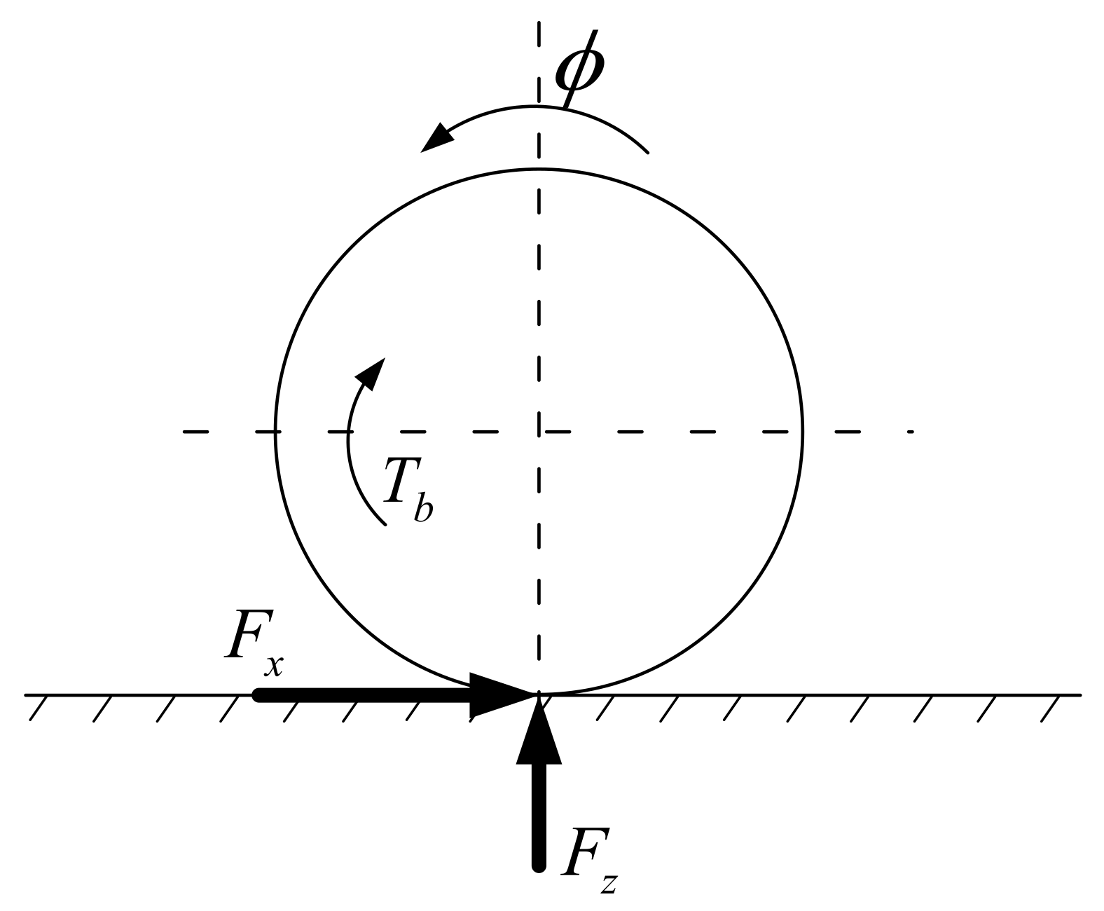
2.1. 2-DOF Vehicle Model

As a simplified non-linear dynamic model for lateral dynamic control, the two-degree-of-freedom (2-DOF) vehicle model, which is displayed in Figure 1 regards the left and right wheels as a whole and can be used to represent the lateral and yaw motion of the vehicles very well [32].

The dynamic equations can be described as follows:

$$\left\{\begin{array}{l}\stackrel{·}{\beta }=\frac{(k_1+k_2)}{m{v}_x}\beta +(\frac{a{k}_1-b{k}_2}{m{v}_x^2}-1)\omega -\frac{k_1}{m{v}_x}{\delta }_f\\ \stackrel{·}{\omega }=\frac{a{k}_1-b{k}_2}{I_z}\beta +\frac{a^2{k}_1+b^2{k}_2}{I_z{v}_x}\omega -\frac{a{k}_1}{I_z}{\delta }_f\end{array}\right.$$

(1)

where $m$ is the mass of the vehicle; the distance from the center of gravity (CG) to front/rear wheel axles are represented by $a$ and $b$; $\beta$ is the sideslip angle of the vehicle; $\omega$ is the yaw rate; $k_1$ and $k_2$ denote the cornering stiffness of the front and rear tires, respectively; $I_z$ is the yaw inertia of vehicle; $v_x$ represents the lateral velocity, and ${\delta }_f$ represents the actual front steering angle.

When the vehicle enters a stable state, its yaw rate can be obtained:

$${\omega }_s=\frac{\frac{v_x}{a+b}}{1+K{v}_x^2}{\delta }_f=\frac{v_x/L}{1+K{v}_x^2}{\delta }_f$$

(2)

Then, we can obtain the sideslip angle at that moment as

$${\beta }_s=\frac{b/L+ma{v}_x{}^2/L^2{k}_2}{1+K{v}_x{}^2}{\delta }_f=(\frac{b}{v_x^2}+\frac{ma}{(a+b)k_2}){\omega }_s{v}_x$$

(3)

where $K$ means the stability factor, $K=\frac{m}{L^2}(\frac{a}{k_2}+\frac{b}{k_1})$.

To prevent vehicle instability, set the upper limit value of yaw rate as

$$\left|{\omega }_{\max }\right|=0.85\frac{\mu g}{v_x}$$

(4)

where $g$ is the gravitational acceleration, $g=9.8 \mathrm{m}/{\mathrm{s}}^2$; $\mu$ is the road adhesion coefficient; the bigger the coefficient, the better the available adhesion, and the less slippery the vehicle will be.

By combining Equations (2) and (4), the desired yaw rate can be expressed as

$${\omega }_{\exp }=\min \left\{\left|{\omega }_s\right|,\left|{\omega }_{\max }\right|\right\}●sign({\omega }_s)$$

(5)

The maximum of the sideslip angle is expressed as

$${\beta }_{\max }=\mu g(\frac{b}{v_x^2}+\frac{ma}{(a+b)k_2})$$

(6)

Combining Equations (3) and (6), we can get the desired sideslip angle as

$${\beta }_{\exp }=\min \left\{\left|{\beta }_s\right|,\left|{\beta }_{\max }\right|\right\}●sign({\beta }_s)$$

(7)

2.2. 7-DOF Vehicle Model

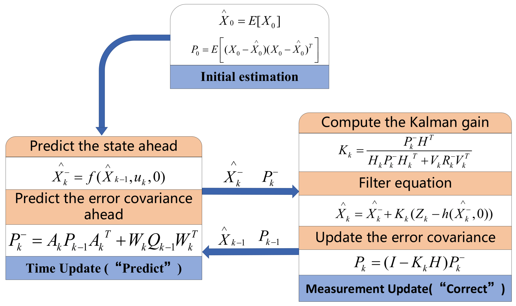
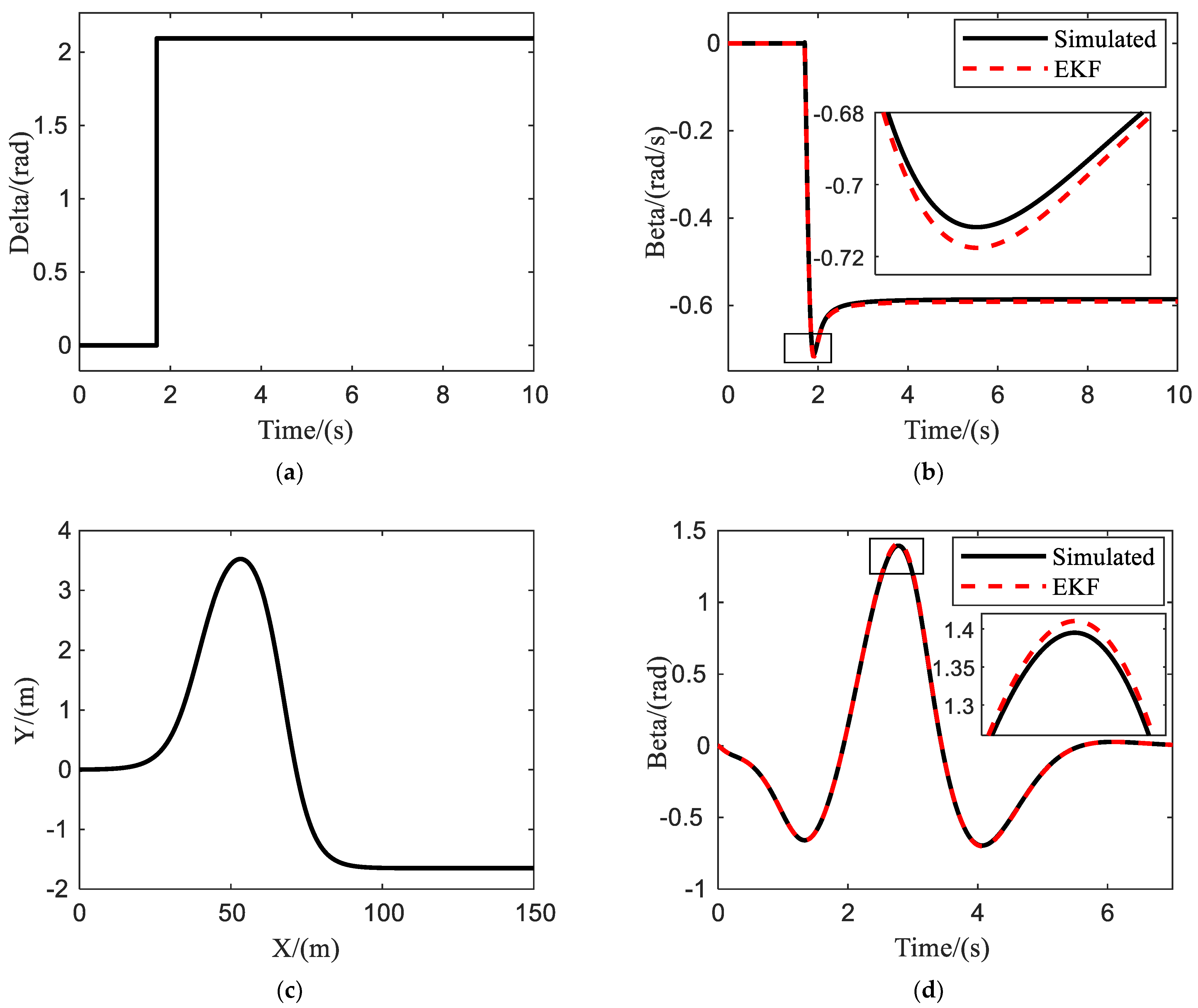
The 2-DOF model only considers the tire cornering characteristics within the linear range; the influence of side wind interference and air resistance on the vehicle during operation is ignored. In addition, the wheels on both sides of the vehicle are considered as a whole, so the yaw moment required by the four wheels of the whole vehicle cannot be obtained. Therefore, a 7-DOF vehicle model consisting of lateral motion and four-wheel rotational motion is chosen to design the DYC controller, which not only considers more degrees of freedom and improves accuracy, but also allows a more realistic simulation of real vehicles. The vehicle model chosen for this section is shown in Figure 2.

Using the following equations, we can describe the longitudinal, lateral, and yaw motions as

$$m{a}_x=F_{x3}+F_{x4}+\left(F_{x1}+F_{x2}\right)\cos {\delta }_f-\left(F_{y1}+F_{y2}\right)\sin {\delta }_f$$

(8)

$$m{a}_y=F_{y3}+F_{y4}+\left(F_{y1}+F_{y2}\right)\cos {\delta }_f +\left(F_{x1}+F_{x2}\right)\sin {\delta }_f$$

(9)

$$\begin{array}{c}{I}_z\dot{\omega }=a\left[\left(F_{x1}+F_{x2}\right)\sin {\delta }_f+\left(F_{y1}+F_{y2}\right)\cos {\delta }_f\right]+\frac{B}{2}\left[\left(F_{x1}-F_{x2}\right)\cos {\delta }_f\right.\\ \left.+\left(F_{y2}-F_{y1}\right)\sin {\delta }_f-(F_{x3}+F_{x4})\right] -b\left(F_{y3}+F_{y4}\right)\end{array}$$

(10)

The external yaw moment $M_z$ can be expressed as

$$M_z=\frac{B}{2}\left(F_{x1}-F_{x2}\right)\cos {\delta }_f+a\left(F_{x1}+F_{x2}\right)\sin {\delta }_f+\frac{B}{2}\left(F_{x4}-F_{x3}\right)\hspace{0.33em}$$

(11)

In the above formulas, $\dot{\omega }$ means the derivative of the actual yaw rate of the vehicle; $F_x$ and $F_y$ represent the longitudinal and lateral forces respectively. For fuel vehicles, $F_x$ depends on the throttle opening; for electric vehicles, it depends on the actual power of the motor. $F_y$ depends on the cornering stiffness of a certain wheel and the sideslip angle of the corresponding wheel.

$$F_y=k●\alpha$$

(12)

where $k$ represents the cornering stiffness of a certain wheel; $\alpha$ means the sideslip angle of the corresponding wheel.

Figure 3 gives a display of the vertical load on each tire, which should be considered when considering how to distribute the additional yaw moment.

where $F_z$ represents the vertical load of the corresponding tire, $F_x$ represents the longitudinal force on the tire, $\varphi$ represents the rotational speed of the tire, $T_b$ means the braking torque.

The vertical loads of each tire are given by

$$\begin{array}{l}{F}_{z1}=\frac{m}{L}\left(\frac{1}{2}g\cdot b-\frac{1}{2}{a}_x\cdot h_g-\frac{b}{B}\cdot a_y\cdot h_g\right)\\ F_{z2}=\frac{m}{L}\left(\frac{1}{2}g\cdot b-\frac{1}{2}{a}_x\cdot h_g+\frac{b}{B}\cdot a_y\cdot h_g\right)\\ F_{z3}=\frac{m}{L}\left(\frac{1}{2}g\cdot a+\frac{1}{2}{a}_x\cdot h_g-\frac{a}{B}\cdot a_y\cdot h_g\right)\\ F_{z4}=\frac{m}{L}\left(\frac{1}{2}g\cdot a+\frac{1}{2}{a}_x\cdot h_g+\frac{a}{B}\cdot a_y\cdot h_g\right)\end{array}$$

(13)

In the above equation, $F_{zi}$ represents the vertical load of the corresponding tire; $F_{xi}$ and $F_{yj}$ represent the longitudinal and lateral forces of each wheel, respectively; $a_x$ and $a_y$ represent the longitudinal and lateral acceleration of the vehicle, respectively; $B$ is the wheelbase of the vehicle, and $h_g$ denotes the height to the center of gravity.

3. EKF Observer

Along with the dramatic improvement of vehicle intelligence and information technology, the requirements for real-time accuracy of vehicle state parameters are also improving. In current mass-produced vehicles, the yaw rate can be accurately measured by sensors, but other vehicle state parameters such as the sideslip angle are still difficult to measure directly due to the high cost of sensors and the limitations of sensor technology. Therefore, EKF technology is applied here to estimate the parameters such as the sideslip angle and to obtain the vehicle state parameters with high calculation accuracy, strong filtering stability and easier engineering implementation.

The Kalman filter works as follows: the filter predicts the state and error covariance at the current moment using the best estimate assessed at the previous moment, then corrects the predicted state value using the measured value at the current moment, and finally calculates the best estimate at this moment, before entering the next cycle. The basic working procedure of the EKF is shown in Figure 4 below.

In Figure 4, in the “Initial estimation” part, ${\stackrel{\wedge }{X}}_0$ means the initial estimation state, $P_0$ represents the initial covariance, $X_0$ is the initial state; in the “Predict” part, $\stackrel{\wedge }{X_k^{-}}$ means the predicted state estimation, $P_k^{-}$ means the predicted error covariance, $A$ is the Jacobian matrix process, and $W$ is the covariance matrix of process noise; in the “Correct” part, $K_k$ represents the Kalman gain matrix, $P_k$ means the updated error covariance, $\stackrel{\wedge }{X_k}$ means the updated state variables.

The EKF is simply linearized for nonlinear systems by performing a first-order Taylor expansion at the filtered optimum that neglects higher-order terms during observation. The state and observation equations of the EKF are constructed using its dynamical equations in conjunction with the developed three-degree-of-freedom vehicle model [33] with nonlinear properties, and the excitation noise characteristics and measurement error characteristics are statistically characterized.

After Taylor series expansion and linearization of the constructed nonlinear equations, the state space equations are shown as follows:

$$\stackrel{·}{x}(t)=f(x(t),u(t),w(t))$$

(14)

$$y(t)=h(x(t),v(t))$$

(15)

where $x(t)$ represents the state variable, $x=[\omega ,\beta ,v_x]$, $u(t)$ represents the control variable, $u={[\delta ,a_x]}^T$, $\delta$ represents the actual front wheel steering angle, $y(t)$ represents the measurement output of the system, $y=[a_y]$; $w(t)$ and $v(t)$ are the mutually independent system excitation noise and measurement noise, respectively, $w=diag{(0.1 0.15 0.13)}^2$, $v=diag{(0.1)}^2$ [34].

Considering that the longitudinal velocity of the vehicle changes in real time when driving, and there is a certain coupling relationship between the longitudinal velocity and the yaw rate, the estimation of the vehicle state in this paper is based on the nonlinear three-degree-of-freedom vehicle model, which considers the yaw motion, side deviation and longitudinal motion of the vehicle. Combined with the nonlinear three-degree-of-freedom vehicle model, the system state equation can be established as follows:

$$\left\{\begin{array}{l}\stackrel{·}{\omega }=\frac{a^2{k}_1+b^2{k}_2}{I_z{v}_x}\omega +\frac{a{k}_1-b{k}_2}{I_z}\beta -\frac{a{k}_1}{I_z}\delta \\ \stackrel{·}{\beta }=(\frac{a{k}_1-b{k}_2}{m{v}_x^2}-1)\omega +\frac{k_1+k_2}{m{v}_x}\beta -\frac{k_1}{m{v}_x}\delta \\ \stackrel{·}{v_x}=a_x+\omega \beta v_x\end{array}\right.$$

(16)

The system measurement equation is given by

$$a_y=\frac{a{k}_1-b{k}_2}{m{v}_x}\omega +\frac{k_1+k_2}{m}\beta -\frac{k_1}{m}\delta$$

(17)

$A$ and $H$ mentioned in Figure 4 are the Jacobi matrices after partial derivatives with $f(x)$ and $h(x)$ functions, respectively:

$$A=\left[\begin{array}{l}\frac{\partial f_1}{\partial x_1}\dots \dots \frac{\partial f_1}{\partial x_m}\\ \dots \dots \dots \dots .\\ \frac{\partial f_m}{\partial x_1}\dots \dots \frac{\partial f_m}{\partial x_m}\end{array}\right]$$

(18)

$$H=\left[\begin{array}{l}\frac{\partial h_1}{\partial x_1}\dots \dots \frac{\partial h_1}{\partial x_m}\\ \dots \dots \dots \dots .\\ \frac{\partial h_m}{\partial x_1}\dots \dots \frac{\partial h_m}{\partial x_m}\end{array}\right]$$

(19)

According to Equations (16) and (17), the below results are obtained.

$$A=\left[\begin{array}{ccc}\frac{a^2{k}_1+b^2{k}_2}{I_z{v}_x}& \frac{a{k}_1-b{k}_2}{I_z}& -\frac{\omega \left(a^2{k}_1+b^2{k}_2\right)}{I_z{v}_x^2}\\ \frac{a{k}_1-b{k}_2}{m{v}_x^2}-1& \frac{k_1+k_2}{m{v}_x}& -\frac{2\left(a{k}_1-b{k}_2\right)\omega }{m{v}_x^3}-\frac{\beta \left(k_1+k_2\right)}{m{v}_x}+\frac{k_1\delta }{m{v}_x^2}\\ \beta v_x& \omega v_x& \omega \beta \end{array}\right]$$

(20)

$$H=\left[\begin{array}{c}\frac{a{k}_1-b{k}_2}{m{v}_x}\\ \frac{k_1+k_2}{m}\\ -\frac{a{k}_1-b{k}_2}{m{v}_x^2}\end{array}\right]$$

(21)

Figure 5 shows the state parameters corresponding to the estimation using EKF and comparing them with the simulation by CarSim, which aims to verify the performance of the designed EKF observer.

The above results are estimated under $v_x=80 \mathrm{k}\mathrm{m}/\mathrm{h}$ and $\mu =0.85$, with two different initial system inputs, designed steering wheel angle and designed path, in which the red curve represents the estimation of the EKF observer, and the black curve represents the actual value simulated by CarSim. From Figure 5a,b, it can clearly be drawn that the sideslip angle of the system can be estimated accurately under the designed steering wheel angle, with its error controlled below 0.9%. Under the designed path, as displayed in Figure 5c,d, the sideslip angle can also be well estimated, whose accuracy can be more than 99%. Therefore, the EKF observer designed in this section can be used to estimate the key state parameters of autonomous vehicles with high accuracy.

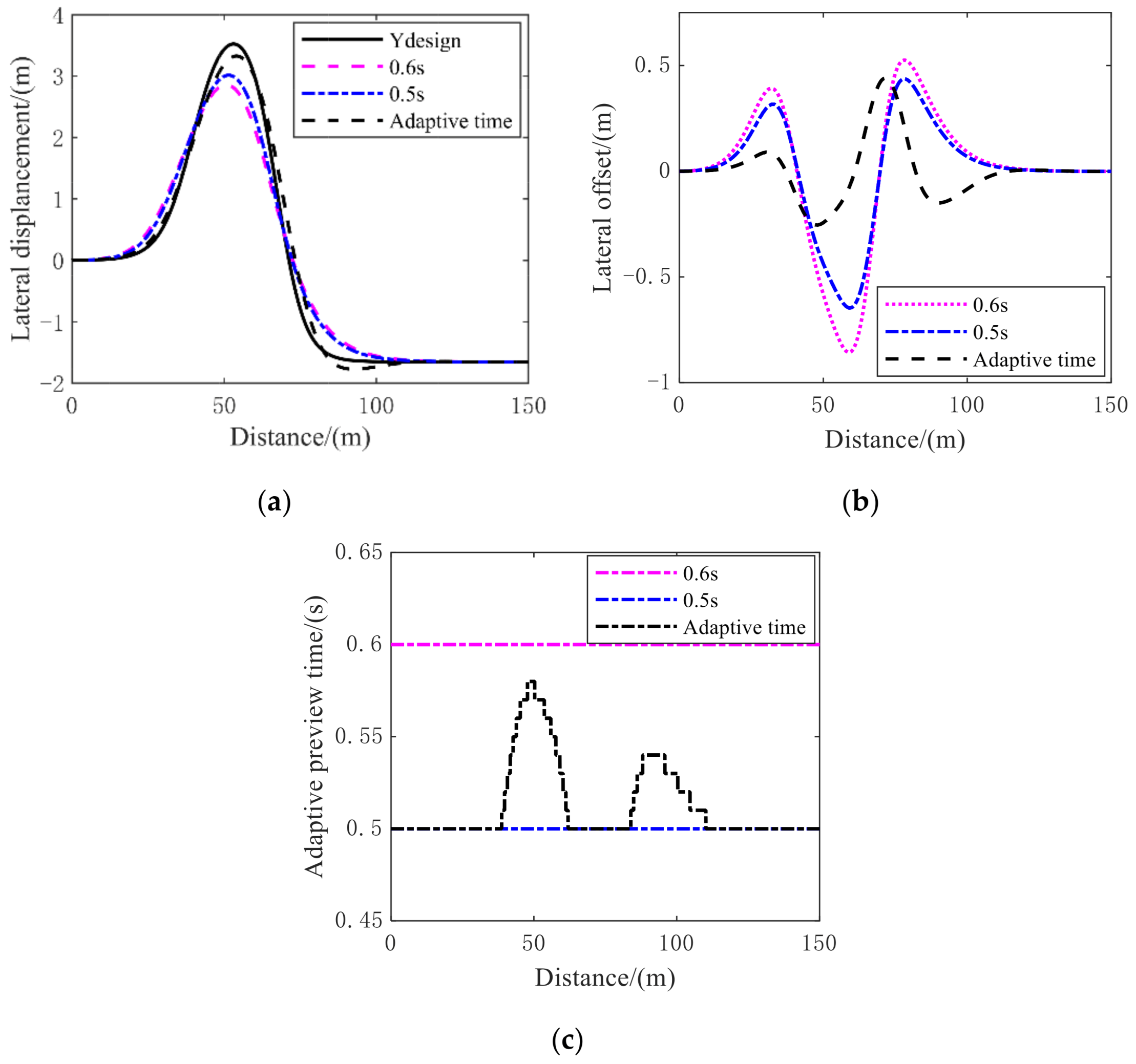
4. Adaptive Preview Time Control

Autonomous vehicles are often faced with complex road traffic environments during actual driving conditions. When the vehicle is driving on a complex trajectory, the length of the preview time has a major connection to vehicle stability. If the preview time is too short, the vehicle is prone to oscillation and driving stability will be reduced in order to follow the reference trajectory. On the other hand, if the preview time is too long, the trajectory-following capability will be easily reduced. Therefore, to overcome this problem, a path-tracking strategy based on adaptive preview time is proposed to enhance the stability and path-following ability of the vehicle while driving complex trajectories.

Consider the preview tracking model [35] shown in Figure 6. Assume that, over a period of time $t_p$, the car maintains a constant yaw rate $\omega$ and because $v_x>>v_y$, the magnitude of the vehicle′s combined velocity $v=\sqrt{v_x{}^2+v_y{}^2}$ can be considered as constant. Given this assumption, the vehicle will follow a uniform circular trajectory with the combined velocity tangential to its path. Figure 6 depicts the target path trajectory of the vehicle, in which the point $M$ denotes the center of gravity at the current moment, and after the elapsed time $t_p$, it will arrive at point $M^{’}$. $X-Y$ is the inertial coordinate system, $X_M-Y_M$ is the vehicle coordinate system, point $P$ represents the preview point on the target path, $L_d$ is the lateral deviation of the preview point, and $MD$ is tangent to the car′s trajectory at point $M$.

From the geometric relationship in Figure 6, we can find the lateral deviation $y_{tp}$ of the point $M^{’}$ during the preview time $t_p$:

$$y_{tp}=\tan (\frac{\theta }{2}+\beta )x_{tp}$$

(22)

Ideally, after the time $t_p$, the vehicle reaches the preview point $P$, at the moment $y_{tp}=L_d$. According to the assumption of uniform yaw motion, the angle that the car has turned within $t_p$ can be describe as $\theta =\omega t_p$. Combine with the displacement of the vehicle in the direction of $X$ axis, $x_{tp}=v_x{t}_p$. Then the desired yaw rate ${\omega }_d$ can be calculated as

$${\omega }_d=2[\arctan (\frac{L_d}{v_x\cdot t_p})-\beta ]/t_p$$

(23)

For the sake of improving the stability and eliminating the influence of the road and driving conditions on real vehicles, we applied a sliding mode controller to generate the yaw rate and verify it in simulation tests. As the control variable, the deviation between the actual and ideal yaw rate is calculated and is used as the sliding mode surface, and the vehicle front wheel angles are chosen as the output variable, with the convergence law used to attenuate the sliding mode jitter. Figure 7 below shows the comparison of the trajectory tracking simulation results under the same vehicle speed conditions with fixed preview times of 0.5 s and 0.6 s and with an adaptive preview time.

From Figure 7a,b, the follow conclusion can be drawn: at the same speed, the vehicle with a fixed preview time does not track the trajectory very well while driving into a curve, and the overall tracking accuracy is not very high; whereas with an adaptive preview time, the reference trajectory can be well tracked, and the vehicle can also find stability more quickly in a curve without oscillation. According to Figure 7b, the mean value of the lateral offset of path tracking based on adaptive preview time decreased by 71.3% of that of 0.5 s, 57.5% of 0.6 s. Figure 7c displays the results of the preview time simulation, where we can find that when driving in a bend, the preview time increases, improving the accuracy of the autonomous vehicle trajectory tracking, and when driving into a straight section, the preview time decreases accordingly, improving driving stability.

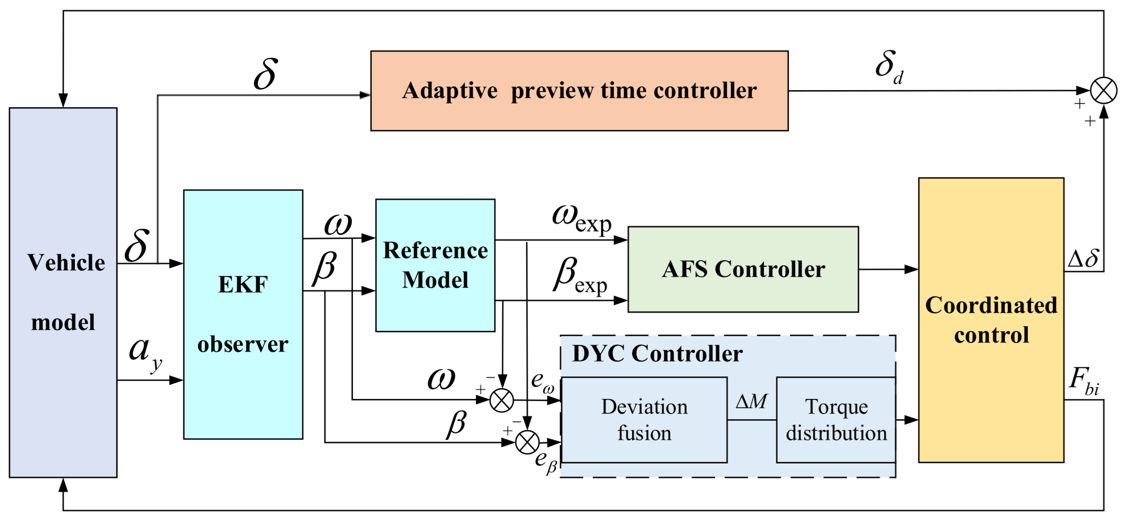
5. Coordinated Control

5.1. AFS Controller Design

When designing the AFS controller, the corresponding equations can be described as

$$\left\{\begin{array}{l}\stackrel{·}{\beta }=\frac{(k_1+k_2)}{m{v}_x}\beta +(\frac{a{k}_1-b{k}_2}{m{v}_x^2}-1)\omega -\frac{k_1}{m{v}_x}({\delta }_f+\Delta \delta )\\ \stackrel{·}{\omega }=\frac{a{k}_1-b{k}_2}{I_z}\beta +\frac{a^2{k}_1+b^2{k}_2}{I_z{v}_x}\omega -\frac{a{k}_1}{I_z}({\delta }_f+\Delta \delta )\end{array}\right.$$

(24)

where ${\delta }_f$ denotes the front wheel angle generated by the steering wheel input; $\Delta \delta$ denotes the additional front wheel angle generated by the active steering controller input.

5.2. DYC Controller Design

Direct yaw-moment control, whose main principle is to achieve stability by changing the engine output power or braking on some wheels, has been widely applied to maintain handling stability of vehicles. Via the 2-DOF vehicle model, the dynamics equations considering the additional yaw moment can be constructed as follows:

$$\left\{\begin{array}{l}\stackrel{·}{\beta }=\frac{(k_1+k_2)}{m{v}_x}\beta +(\frac{a{k}_1-b{k}_2}{m{v}_x^2}-1)\omega -\frac{k_1}{m{v}_x}{\delta }_f\\ \stackrel{·}{\omega }=\frac{a{k}_1-b{k}_2}{I_z}\beta +\frac{a^2{k}_1+b^2{k}_2}{I_z{v}_x}\omega -\frac{a{k}_1}{I_z}{\delta }_f+\frac{\Delta M}{I_z}\end{array}\right.$$

(25)

where $\Delta M$ represents the additional yaw moment.

A sliding mode controller is proposed, with the corresponding control system block diagram in Figure 8 showing how it meets the function of DYC.

5.2.1. DYC Controller

In order to adapt to various driving scenarios and enhance stability while tracking the trajectory, a sliding mode controller based on joint control between $\omega$ and $\beta$ is proposed, where $e_{\omega }$ and $e_{\beta }$ are the system inputs and the additional yaw moment $\Delta M$ is chosen as the output. Dimensional analysis is considered in this section, with the yaw rate deviation $e_{\omega }$ and the sideslip angle error $e_{\beta }$ will be dimensionless by using the threshold method. By reducing the number of inputs, the dimensionality of the controller is reduced, simplifying the control system structure and reducing the computational effort of the control system to a certain extent. The detailed operation steps are as follows:

First, two critical parameters, $e_{\omega }$ and $e_{\beta }$ will be dimensionless according to the extremum method [36] with the following equations:

$${\overline{e}}_{\omega }=1-\frac{e_{\omega }-e_{\omega \min }}{e_{\omega \max }-e_{\omega \min }}$$

(26)

$${\overline{e}}_{\beta }=1-\frac{e_{\beta }-e_{\beta \min }}{e_{\beta \max }-e_{\beta \min }}$$

(27)

where ${\overline{e}}_{\omega }$ and ${\overline{e}}_{\beta }$ are the dimensionless deviations of the yaw rate and the sideslip angle; $e_{\omega \max }$ and $e_{\omega \min }$ represent the maximum and minimum values of the yaw rate deviation, respectively; $e_{\beta \max }$ and $e_{\beta \min }$ represent the maximum and minimum values of the sideslip angle, respectively.

Then, by weighting and summing the two Equations (26) and (27), the following equations are obtained, where a comprehensive deviation $E$ is achieved as

$$E=\epsilon {\overline{e}}_{\omega }+(1-\epsilon ){\overline{e}}_{\beta }$$

(28)

where $\epsilon$ represents the weight coefficient, $0<\epsilon <1$, and the value of $\epsilon$ is related to $\omega$ and $\beta$, representing the proportion of both in the total error.

The slip surface can be simplified by formulating it as

$$s_{\omega -\beta }=K_{i}E$$

(29)

where $K_i$ is a positive number.

To find the first order derivative of Equation (29), substitute Equation (11) to obtain the following equation:

$$\begin{array}{l}{\dot{s}}_{\omega -\beta }=K_i\dot{E}\\ =\frac{{\Upsilon }_1}{I_z{\partial }_1}\left[a\left(F_{y1}+F_{y2}\right)\cos {\delta }_f+\frac{B}{2}\left(F_{y2}-F_{y1}\right)\sin {\delta }_f\right.\left.-b\left(F_{y4}+F_{y3}\right)+\Delta M\right]-\frac{{\Upsilon }_1}{{\partial }_1}({\dot{\omega }}_{\exp }+e_{\omega \min })\\ + \frac{{\Upsilon }_2}{{\partial }_2}(\dot{\beta }-{\dot{\beta }}_{\exp }-e_{\beta \min })\end{array}$$

(30)

where ${\Upsilon }_1=K_i\epsilon$, ${\partial }_1=e_{\omega \max }-e_{\omega \min }$, ${\Upsilon }_2=(1-\epsilon )K_i$, ${\partial }_2=e_{\beta \max }-e_{\beta \min }$.

Let ${\dot{s}}_{w-\beta }=0$, and the equivalent control law for the transverse pendulum moment is given by

$$\begin{array}{l}{M}_{eq}=-\left[a\left(F_{y1}+F_{y2}\right)\cos {\delta }_f+\frac{B}{2}\left(F_{y2}-F_{y1}\right)\sin {\delta }_f\right.\left.-b\left(F_{y4}+F_{y3}\right) -I_z({\dot{\omega }}_{\exp }+e_{\omega \min })\right]\\ + \frac{{\partial }_1{\Upsilon }_2}{{\partial }_2{\Upsilon }_1}{I}_z(\dot{\beta }-{\dot{\beta }}_{\exp }-e_{\beta \min })\end{array}$$

(31)

By applying a modified convergence law, the tracking rate and accuracy can be dramatically improved, and the jitter that occurs with sliding mode control will be quickly suppressed. The referred law can be expressed as:

$$\dot{s}=-{\gamma }_1{\left|s\right|}^n\mathrm{sgn}\left(s\right)-{\gamma }_2{\left|s\right|}^n\mathrm{sgn}\left(s\right)-{\gamma }_{3}s$$

(32)

where $n$ is the coefficient of power reaching law, $0<n<1$.

Combining Equations (31) and (32), the final output of the direct yaw moment controller can be obtained as

$$\Delta M=M_{eq}-{\gamma }_1{\left|s_{\omega -\beta }\right|}^n\mathrm{sgn}\left(s_{\omega -\beta }\right)-{\gamma }_2{\left|s_{\omega -\beta }\right|}^n\mathrm{sgn}\left(s_{\omega -\beta }\right) -{\gamma }_3{s}_{\omega -\beta }$$

(33)

5.2.2. Stability Analysis

Theorem 1.

The controller formulated in Equation (33) will be asymptotically stable in finite time under Lyapunov theory.

Proof. 

Substitution of Equation (33) into Equation (30) yields.

$${\dot{s}}_{\omega -\beta }=-\frac{{\Upsilon }_1}{I_z{\partial }_1}\left[ {\gamma }_1{\left|s_{\omega -\beta }\right|}^n\mathrm{sgn}\left(s_{\omega -\beta }\right)+{\gamma }_2{\left|s_{\omega -\beta }\right|}^n\mathrm{sgn}\left(s_{\omega -\beta }\right)\right.\left.+{\gamma }_3{s}_{\omega -\beta }\right]$$

(34)

A Lyapunov function can be defined as

$$V=\frac{1}{2}{s}^2$$

(35)

Differentiating the Lyapunov function (35) yields

$$\begin{array}{l}\dot{V}=s_{\omega -\beta }{\dot{s}}_{\omega -\beta }\\ =-\frac{{\Upsilon }_1}{I_z{\partial }_1}\left[{\gamma }_1{\left|s_{\omega -\beta }\right|}^n{s}_{\omega -\beta }\mathrm{sgn}\left(s_{\omega -\beta }\right)\right.+ \left.{\gamma }_2{\left|s_{\omega -\beta }\right|}^n{s}_{\omega -\beta }\mathrm{sgn}\left(s_{\omega -\beta }\right)+{\gamma }_3{s}_{\omega -\beta }{}^2\right]\end{array}$$

(36)

where $s_{\omega -\beta }\ne 0$, with$s_{\omega -\beta }{}^2>0$, $\dot{V}<0$ can be deduced because $\mathrm{sgn}\left(s_{\omega }\right)s_{\omega }>0$, and as a result of this, a steady state can be predicted for the sliding mode surface. This shows that the system satisfies the stability requirements and is stable in the Lyapunov sense, and Theorem 1 is proved. □

5.2.3. Yaw Moment Distribution Strategy

The purpose of the DYC system is to make the vehicle maintain a stable state by sensing in advance whether there is a tendency for the vehicle to drift or skid in extreme danger and by taking proactive action to prevent the driver from making a panicked error. When a vehicle is detected to be in a state of instability, the controller immediately calculates the additional force required to stabilize the vehicle, but the additional transverse moment generated cannot be applied directly to the wheels and needs to be converted into a longitudinal force (drive/braking force) applied to each wheel using a lower-level torque distribution strategy.

In view of the smooth vehicle state transition and low impact during single wheel braking control, the driving comfort of the occupants is better. Meanwhile, single-wheel braking can react more quickly and feed the requirements of the controller much better compared to dual-wheel braking, which means it can quickly respond to the controller and save much more time. Therefore, a single-wheel braking control strategy is chosen in this section. By confirming the positive and negative values of current ${\overline{e}}_{\omega }$ and the direction of the front wheel angle, the corresponding wheel for braking can be selected. The yaw moment control strategy is shown in

Table 1. DYC distribution strategy.

Vehicle Orientation	Vehicle Status	${\overline{\mathit{e}}}_{\mathit{\omega }}$	Brake Wheel Chosen	The Braking Torque
Turn left	$K>0$ (Understeering)	+	Left rear	$T_{b1}=F_{b1}\cdot R$ $F_{b1}=\frac{\Delta M}{-B/2\cdot \cos {\delta }_f+a\sin {\delta }_f}$
	$K<0$ (Oversteering)	−	Right front	$T_{b2}=F_{b2}\cdot R$ $F_{b2}=\frac{\Delta M}{-B/2\cdot \cos {\delta }_f+a\sin {\delta }_f}$
Turn right	$K>0$ (Understeering)	+	Left front	$T_{b3}=F_{b3}\cdot R$ $F_{b3}=\frac{\Delta M}{B/2}$
	$K<0$ (Oversteering)	−	Right rear	$T_{b4}=F_{b4}\cdot R$ $F_{b4}=\frac{\Delta M}{B/2}$

.

Finally, the values of the moments obtained need to be constrained as

$$T_{bi}=\left\{\begin{array}{c}{T}_{bi} T_{\max }\le \mu R{F}_{zi}\\ \mu R{F}_{zi} T_{\max }> \mu R{F}_{zi} \end{array}\right.$$

(37)

where $F_{zi}$ and $T_{bi}$ represent the vertical load and braking torque on individual wheels, $T_{\max }$ represents the maximum torque output and $R$ represents the radius of tire.

5.3. AFS and DYC Coordinated Control

To determine the driver′s maneuvering intentions and ensure the vehicle is stable while driving, the AFS and DYC systems need to function optimally in their respective operating areas, which can further decrease the impact of braking action on longitudinal dynamics and ensure a comfortable driving experience. In this paper, coordinated control is chosen to implement the integrated design of AFS and DYC controllers.

Figure 9 displays the overall architecture of the coordinated controller, where we use the 2-DOF vehicle model as the reference model and obtain the desired yaw rate ${\omega }_{\exp }$ and the desired sideslip angle ${\beta }_{\exp }$.

The key to coordinated control lies in the allocation and coordinated work between the two systems, so on the one hand, the recognition rate of the determination module should be improved to reduce the occurrence of misjudgment situations; on the other hand, the cut-in timing of DYC should be determined. Based on this section, the critical steering angle and allocation algorithm are designed, and the respective weight coefficients of AFS and DYC are calculated by confirming vehicle status, aiming to divide the respective working areas of the two systems, avoiding the sudden intervention of DYC and taking the vehicle handling stability and driving comfort into account.

5.3.1. Critical Steering Angle

To determine the intervention time of the DYC controller, simulation experiments were carried out, and the critical steering angle of the front wheels were determined through phase-plane analysis theory [37]. A 2-DOF vehicle model was constructed in the software MATLAB/Simulink with longitudinal velocity, steering angle and road adhesion coefficient as control inputs; the CarSim-Simulink co-simulation will be able to determine the critical steering angle for different velocities and road surfaces with different adhesion coefficients, which are displayed in the table below.

By analyzing

Table 2. Table of critical steering angles of different velocities and road adhesion coefficients.

Velocity/(km/h)	Road Adhesion Coefficient	Critical Front Wheel Angle/(°)
60	0.2	1.625
90	0.2	1.125
120	0.2	0.625
60	0.5	3.125
90	0.5	1.375
120	0.5	1.125
60	0.8	4.875
90	0.8	2.125
120	0.8	1.375

and Figure 10, the following conclusion can be obtained: with the increase in vehicle velocity and the decrease in the road adhesion coefficient, the critical front wheel steering angle will decrease. Through MATLAB, the approximate value of the critical steering angle can be calculated, whose formula is expressed as follows:

$${\delta }_i=5.7037+0.00064815v_x{}^2-0.9259{\mu }^2-0.1181v_x-8.1019\mu -0.0694v_x\cdot \mu$$

(38)

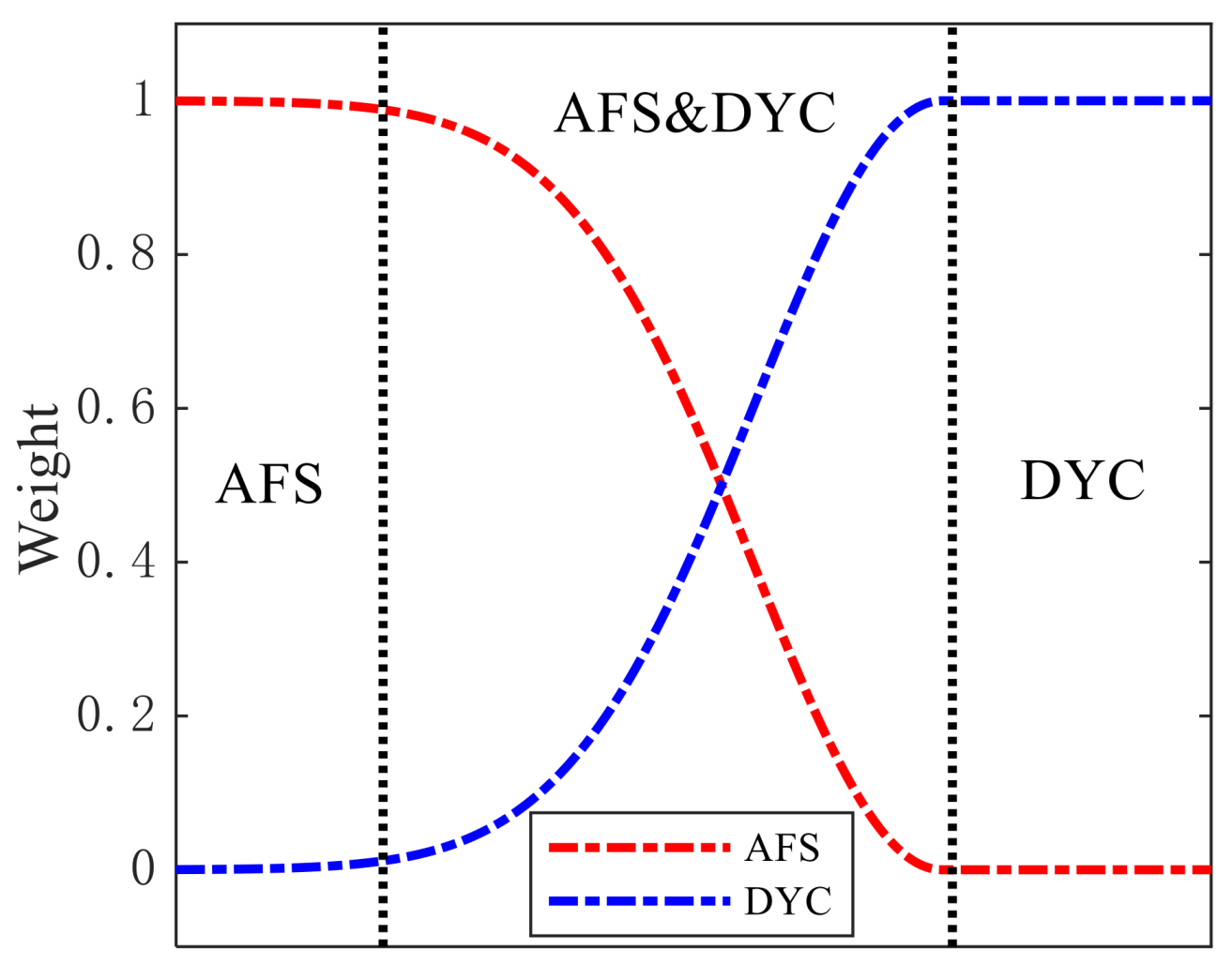
5.3.2. Switching Function

Under the critical stability state, the vehicle will face the problem of switching from AFS to DYC [30]. If the switching speed is too fast, the vehicle will easily become unstable and the driver and passengers will be very uncomfortable; meanwhile, if the switching speed is too slow, the vehicle will enter an unstable state and become dangerous. Therefore, it is necessary to design an appropriate switching function when the front wheel is turning to the critical steering angle and fully consider the intervention moment of each system to maintain stability and ensure a comfortable driving experience.

A switching function [38] is shown as follows:

$$y=\frac{1}{e^{\frac{1}{2{\xi }^2}\left(\frac{{\delta }_f-{\delta }_i}{{\delta }_i}\right)}{}^{{}^{{}^{{}^{{}^{{}^2}}}}}}$$

(39)

where ${\delta }_f$ represents the actual front wheel angle; ${\delta }_i$ represents the critical steering angle calculated under the corresponding working condition; $\xi$ is an adjustment coefficient of this function and is assigned as 0.135.

When the AFS is fully output, the weighting factor is $p=1$; when the DYC is fully output, the weighting factor is $1-p=1$; the coordinated allocation is added to Equation (39), which gives the output of the AFS system $\Delta {\delta }_f{}^{’}=p\Delta {\delta }_f$ and the output of the DYC system $M_z{}^{’}=(1-p)M_z$. This has the effect that the intervention of the DYC control and the exit of the AFS control is a gradual process, avoiding shocks to the system. The value of the specific weighting parameter is displayed in the following formula:

$$p=\left\{\begin{array}{cc}0,\hfill & {\delta }_i-\left|{\delta }_f\right|>L_f\hfill \\ \frac{1}{\frac{1}{2{\xi }^2}{\left(\frac{{\delta }_f-{\delta }_i}{{\delta }_i}\right)}^2},\hfill & {\delta }_i-\left|{\delta }_f\right|<L_f\hfill \\ 1,\hfill & \left|{\delta }_i-{\delta }_f\right|<L_f\hfill \end{array}\right.$$

(40)

where $L_f$ represents the boundary value of the coordination region, $\left|L_f\right|\le {0.8}^{\circ }$.The graph of the switching function is shown in Figure 11.

6. Simulation and Discussion

In order to verify the effectiveness of the coordinated control strategy proposed in this paper, two kinds of driving conditions of the vehicle under high-speed conditions and low-adhesion coefficient conditions were simulated and tested, respectively. Firstly, the simulation environment and control module, such as adaptive preview time module, AFS controller and DYC controller, are established in Simulink according to the above sections, and the relevant parameters of the vehicle are modified in CarSim and the corresponding working conditions are designed or selected in the road setting interface. The three strategies were carried out respectively to compare their control performance. The vehicle parameters applied in the simulation are shown in the following

Table 3. Vehicle simulation parameters.

Parameter Name	Value	Unit
Vehicle mass	1412	$\mathrm{k}\mathrm{g}$
Distance of the front axle from CG	1.015	$\mathrm{m}$
Distance of the rear axle from CG	1.895	$\mathrm{m}$
Height of gravity center	0.65	$\mathrm{m}$
Cornering stiffness of the front wheel	112,600	$\mathrm{N}/\mathrm{r}\mathrm{a}\mathrm{d}$
Cornering stiffness of the front wheel	112,600	$\mathrm{N}/\mathrm{r}\mathrm{a}\mathrm{d}$
Wheelbase	1.675	$\mathrm{m}$
Wheel rolling radius	0.325	$\mathrm{m}$
Yaw moment of inertia	1536.7	$\mathrm{k}\mathrm{g}/{\mathrm{m}}^2$

.

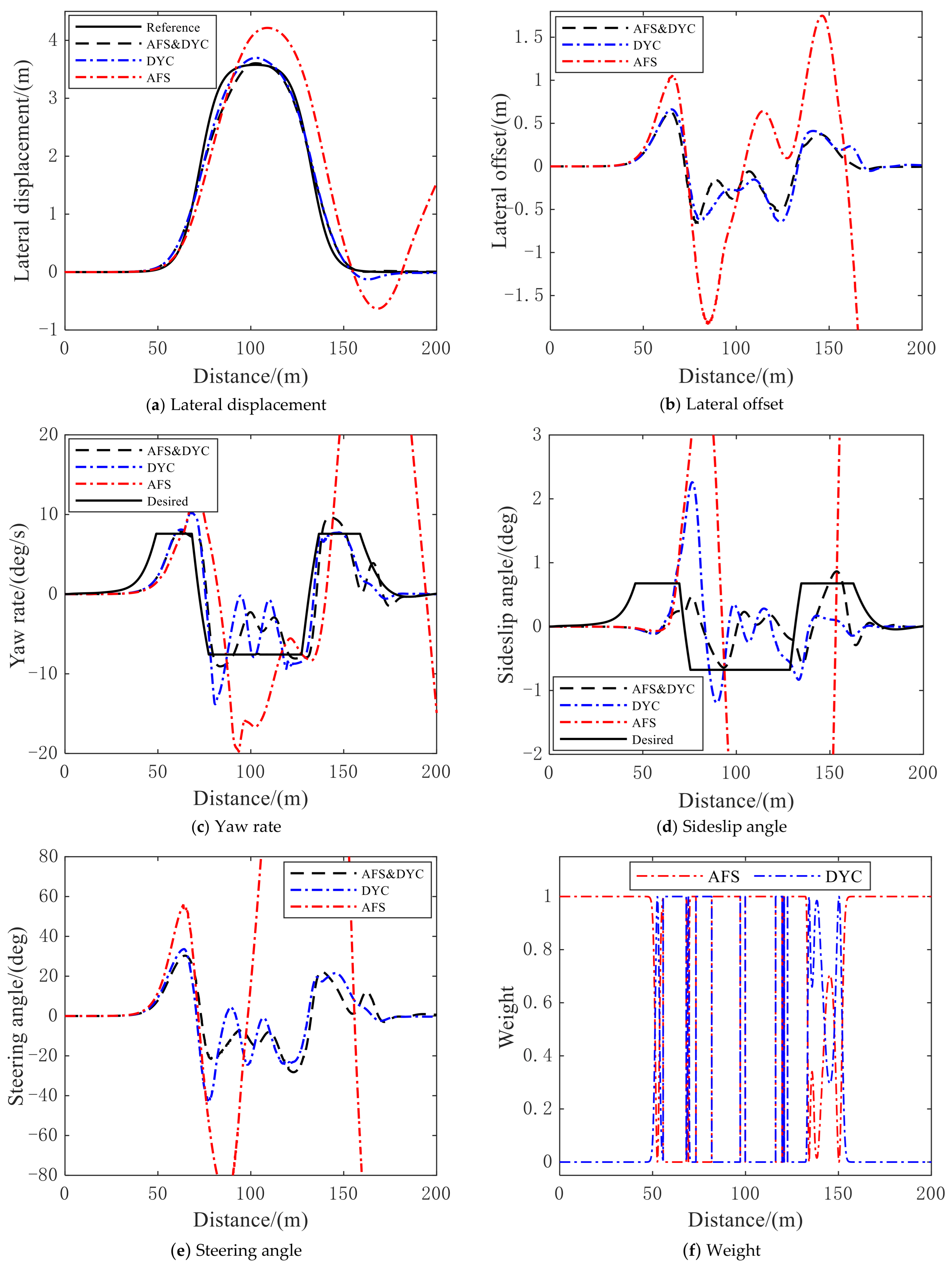
6.1. Simulation under High-Speed Driving Conditions

In this section, FHWA lane in CarSim is selected as the reference trajectory for path tracking to verify the control effect of three controllers under high-speed driving conditions. The simulated longitudinal speed is set to 110 km/h, with the adhesion coefficient set to 0.85. Performance of the lateral stability and path-tracking accuracy of the vehicle is observed at a high speed with AFS control alone, DYC control alone and coordinated control, and some critical variables, such as lateral offset, yaw rate, sideslip angle and so on, are displayed.

The path-tracking accuracy and driving stability can be inferred from Figure 12.

As can be seen from Figure 12a, when the speed reaches 110 km/h, the vehicle cannot be stabilized by only relying on AFS control alone, while the vehicle under DYC and coordinated control completes the simulation very well.

By comparing the lateral error in Figure 12b, it is obvious that the vehicle under coordinated control of AFS and DYC has the best path-tracking accuracy, and its stability is also outstanding compared to the separate controllers. Figure 12c–e show the yaw rate, the sideslip angle and the lateral acceleration of the vehicles. The AFS system, which works by adjusting the front wheel steering angle, has reached its limitation, and the lateral deflection force of the tire has reached the maximum and turned to the nonlinear region, leading to a loss of its stability. The DYC system controls the longitudinal force of the vehicle, so the longitudinal velocity will change when DYC works, and thus the stability will be affected, as shown by its yaw rate and sideslip angle. The vehicle stability is affected by critical parameters—yaw rate and sideslip angle—which may lead to poor handling experience and comfort for the driver and passengers during the actual maneuvering, but its overall control effect is satisfactory, and the vehicle maintains its stability through the whole simulation. The coordinated control of AFS and DYC, under the same vehicle conditions and road conditions, can fully utilize the longitudinal and lateral ground adhesion of the tires, so its overall parameters are more stable and do not show large fluctuations, and its yaw rate, sideslip angle and lateral acceleration are better than those under AFS and DYC control alone. Taking the yaw rate as an example, the following conclusions can be obtained by comparing the data: under the high-speed FHWA conditions, the maximum value of the yaw rate under coordinated control of AFS and DYC can be reduced by 30.3%, the minimum value was reduced by 14.3%, and the standard deviation was reduced by 8.0% compared with DYC. Therefore, it is reasonable that in actual control, coordinated control will achieve better tracking accuracy and ensure better stability and ride comfort. Figure 12f shows the switching progress and weight of AFS and DYC, which verifies that the coordinated control comprehensively utilizes the advantages of AFS and DYC and eventually reaches the best performance.

Table 4. Yaw rate under high-speed conditions.

$\mathit{\omega }/(\mathbf{deg}/\mathit{s})$	Maximum	Minimum	Range	Std. Deviation
DYC	15.53	−9.578	25.11	5.73
AFS&DYC	10.83	−8.209	19.03	5.273

and

Table 5. Sideslip angle under high-speed conditions.

$\mathit{\beta }/(\mathbf{deg})$	Maximum	Minimum	Range	Std. Deviation
DYC	2.022	−0.5435	2.565	0.3999
AFS&DYC	0.6659	−0.406	1.072	0.1955

display the yaw rate and sideslip angle under high-speed conditions respectively.

Overall, the test under high speed verifies that the coordinated control of AFS and DYC has better path-tracking performance and simultaneously achieves superior driving stability than separate controls.

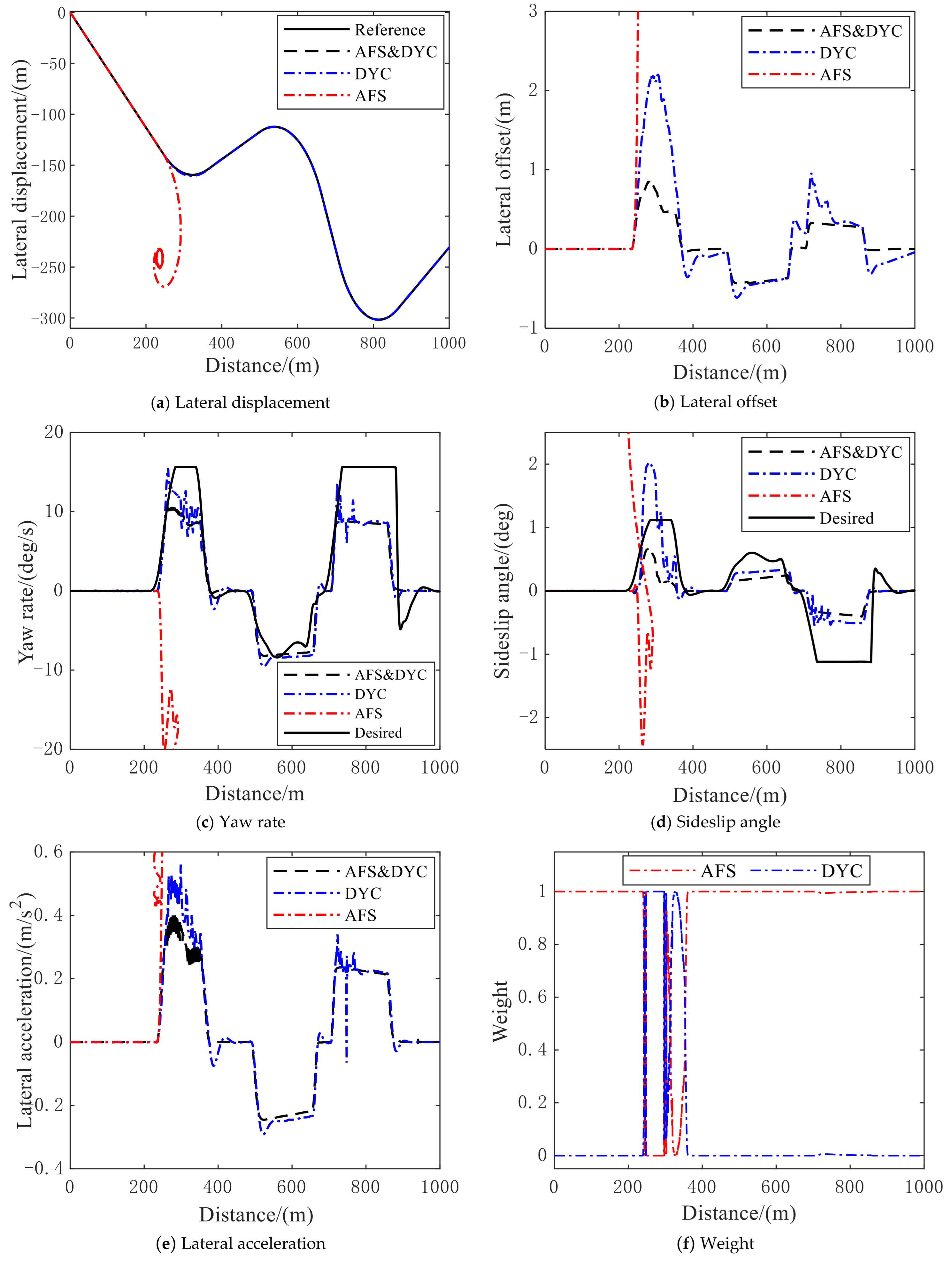
6.2. Simulation under Low Adhesion Coefficient

In this section, we choose the double lane change maneuver as the reference trajectory for path tracking and observe the accuracy and the lateral performance of the vehicle under AFS, DYC and coordinated control when the vehicle is driving under a low adhesion coefficient road. The simulation speed is set to 80 km/h and the road adhesion coefficient is set to 0.3. The simulation results are shown in Figure 13.

As can be seen in Figure 13, the simulations of the vehicle under double lane change show different effects under a low adhesion coefficient road, in which the vehicle under AFS and DYC coordinated control has relatively better path tracking and lateral stability performance.

Because of the low adhesion coefficient of the road, the lateral deflection force of the tires will easily reach saturation, and the vehicle will move far away from the reference path under AFS control. In addition, from Figure 13b, we can also see that the vehicle has the biggest offset when controlled by the AFS system, while coordinated control can obtain the best tracking accuracy. Figure 13c–e show how the yaw rate, the sideslip angle and the steering angle of the vehicle change during the whole performance. Due to the control of longitudinal force, the longitudinal velocity under DYC control will change, which will affect the stability of the vehicle, with its yaw rate, sideslip angle and steering angle a large fluctuation, and eventually contribute to the poor handling experience and drive comfort. The vehicle under the coordinated control can take the lateral force of the wheels into account and adjust the longitudinal force in time so that the path-tracking performance and driving stability can always maintain a better control ability, and its yaw rate and sideslip angle can be kept stable. Taking the sideslip angle as an example, using the statistical information in MATLAB, the following conclusions can be drawn: under low adhesion coefficient conditions, the maximum value of the sideslip angle of coordinated control is reduced by 67.1%, the minimum value is reduced by 25.6%, and the standard deviation is reduced by 51.1% compared to the DYC control. Figure 13f shows how the coordinated control switches between AFS and DYC and maintains the stability of the vehicle.

Table 6. Yaw rate under low adhesion coefficient.

$\mathit{\omega }/(\mathbf{deg}/\mathit{s})$	Maximum	Minimum	Range	Std. Deviation
DYC	10.28	−13.82	24.09	4.907
AFS&DYC	9.656	−9.065	18.72	4.651

and

Table 7. Sideslip angle under low adhesion coefficient.

$\mathit{\beta }/(\mathbf{deg})$	Maximum	Minimum	Range	Std. Deviation
DYC	2.022	−0.5435	2.565	0.3999
AFS&DYC	0.6659	−0.406	1.072	0.1955

display the yaw rate and sideslip angle under low adhesion coefficient. respectively.

The DLC simulation shows that the coordinated control of AFS and DYC makes good use of the ground adhesion, and its tracking performance is better than that of AFS or DYC alone, which can guarantee vehicle stability and obtain better tracking accuracy at the same time.

7. Conclusions and Prospects

In this paper, we propose a coordinated control system based on state estimation and path tracking, which aims to ensure driving stability and improve the path-tracking capability of autonomous vehicles under complex and dynamic road conditions.

(1)

An EKF observer is designed to estimate the sideslip angle, aiming to better investigate the lateral stability performance of autonomous vehicles.

(2)

Path-tracking accuracy is optimized based on the adaptive preview time controller, and the vehicle tracks the reference trajectory well and can meet the driving requirements of turning and straight driving conditions.

(3)

An AFS and DYC coordinated control strategy is designed by considering the cut-in moment, and the simulation results demonstrate that the controller makes good use of the road adhesion, and its tracking performance is better than that of AFS or DYC alone, which can ensure the stability of the vehicle and obtain better tracking accuracy simultaneously.

In fact, the influence of path curvature on tracking accuracy in trajectory tracking is ignored, and the performance of path tracking and stability control under acceleration should be considered theoretically. Also, the road surface adhesion coefficient should be classified to adapt to different road conditions and improve the robustness of the system.

References

1. Nam, K.; Fujimoto, H.; Hori, Y. Lateral Stability Control of In-Wheel-Motor-Driven Electric Vehicles Based on Sideslip Angle Estimation Using Lateral Tire Force Sensors. IEEE Trans. Veh. Technol. 2012, 61, 1972–1985. [Google Scholar] [CrossRef]
2. Zhou, B.; Xu, M.; Fan, L.; Yuan, X. Integrated control for AFS and EPS with EKF estimation of lateral force. J. Vib. Shock. 2015, 34, 93–98. [Google Scholar] [CrossRef]
3. Hang, P.; Chen, X. Integrated chassis control algorithm design for path tracking based on four-wheel steering and direct yaw-moment control. Proc. Inst. Mech. Eng. Part I J. Syst. Control. Eng. 2019, 233, 625–641. [Google Scholar] [CrossRef]
4. Chindamo, D.; Lenzo, B.; Gadola, M. On the Vehicle Sideslip Angle Estimation: A Literature Review of Methods, Models, and Innovations. Appl. Sci. 2018, 8, 355. [Google Scholar] [CrossRef]
5. Chen, T.; Chen, L.; Xu, X.; Cai, Y.; Jiang, H.; Sun, X. Sideslip Angle Fusion Estimation Method of an Autonomous Electric Vehicle Based on Robust Cubature Kalman Filter with Redundant Measurement Information. World Electr. Veh. J. 2019, 10, 34. [Google Scholar] [CrossRef]
6. Gapiński, D.; Koruba, Z. Control of Optoelectronic Scanning and Tracking Seeker by Means the LQR Modified Method with the Input Signal Estimated Using of the Extended Kalman Filter. Energies 2021, 14, 3109. [Google Scholar] [CrossRef]
7. Amer, N.H.; Zamzuri, H.; Hudha, K.; Petrou, L. Modelling and Control Strategies in Path Tracking Control for Autonomous Ground Vehicles: A Review of State of the Art and Challenges. J. Intell. Robot. Syst. 2017, 86, 225–254. [Google Scholar] [CrossRef]
8. Yao, Q.; Tian, Y.; Wang, Q.; Wang, S. Control Strategies on Path Tracking for Autonomous Vehicle: State of the Art and Future Challenges. IEEE Access 2020, 8, 161211–161222. [Google Scholar] [CrossRef]
9. Zhao, P.; Chen, J.; Song, Y.; Tao, X.; Xu, T.; Mei, T. Design of a Control System for an Autonomous Vehicle Based on Adaptive-PID. Int. J. Adv. Robot. Syst. 2012, 9, 44. [Google Scholar] [CrossRef]
10. Chen, J.; Zhu, H.; Zhang, L.; Sun, Y. Research on fuzzy control of path tracking for underwater vehicle based on genetic algorithm optimization. Ocean Eng. 2018, 156, 217–223. [Google Scholar] [CrossRef]
11. Wang, H.; Liu, B.; Ping, X.; An, Q. Path Tracking Control for Autonomous Vehicles Based on an Improved MPC. IEEE Access 2019, 7, 161064–161073. [Google Scholar] [CrossRef]
12. Imine, H.; Madani, T. Sliding-mode control for automated lane guidance of heavy vehicle. Int. J. Robust Nonlinear Control. 2013, 23, 67–76. [Google Scholar] [CrossRef]
13. Akermi, K.; Chouraqui, S.; Boudaa, B. Novel SMC control design for path following of autonomous vehicles with uncertainties and mismatched disturbances. Int. J. Dyn. Control. 2020, 8, 254–268. [Google Scholar] [CrossRef]
14. Wang, L.; Zhu, S.; Liu, Y.; Du, X.; Zhu, Z.; Zhai, Z. A novel path tracking method of tractor based on improved second-order sliding mode considering front wheel steering angle compensation. Proc. Inst. Mech. Eng. Part D J. Automob. Eng. 2022. [Google Scholar] [CrossRef]
15. Han, G.; Fu, W.; Wang, W.; Wu, Z. The Lateral Tracking Control for the Intelligent Vehicle Based on Adaptive PID Neural Network. Sensors 2017, 17, 1244. [Google Scholar] [CrossRef]
16. Zhang, X.; Zhu, X. Autonomous path tracking control of intelligent electric vehicles based on lane detection and optimal preview method. Expert Syst. Appl. 2019, 121, 38–48. [Google Scholar] [CrossRef]
17. Cho, J.; Huh, K. Active Front Steering for Driver’s Steering Comfort and Vehicle Driving Stability. Int. J. Automot. Technol. 2019, 20, 589–596. [Google Scholar] [CrossRef]
18. Wu, Y.; Wang, L.; Zhang, J.; Li, F. Robust vehicle yaw stability control by active front steering with active disturbance rejection controller. Proc. Inst. Mech. Eng. Part I J. Syst. Control. Eng. 2019, 233, 1127–1135. [Google Scholar] [CrossRef]
19. Sun, P.; Trigell, A.S.; Drugge, L.; Jerrelind, J. Energy efficiency and stability of electric vehicles utilising direct yaw moment control. Veh. Syst. Dyn. 2022, 60, 930–950. [Google Scholar] [CrossRef]
20. Fu, C.; Hoseinnezhad, R.; Li, K.; Hu, M. A novel adaptive sliding mode control approach for electric vehicle direct yaw-moment control. Adv. Mech. Eng. 2018, 10, 1–12. [Google Scholar] [CrossRef]
21. Wu, J.; Cheng, S.; Liu, B.; Liu, C. A Human-Machine-Cooperative-Driving Controller Based on AFS and DYC for Vehicle Dynamic Stability. Energies 2017, 10, 1737. [Google Scholar] [CrossRef]
22. Sun, T.; Guo, H.; Cao, J.-Y.; Chai, L.-J.; Sun, Y.-D. Study on Integrated Control of Active Front Steering and Direct Yaw Moment Based on Vehicle Lateral Velocity Estimation. Math. Probl. Eng. 2013, 2013, 1–8. [Google Scholar] [CrossRef]
23. Ding, N.; Taheri, S. An adaptive integrated algorithm for active front steering and direct yaw moment control based on direct Lyapunov method. Veh. Syst. Dyn. 2010, 48, 1193–1213. [Google Scholar] [CrossRef]
24. Zhao, J.; Wong, P.K.; Ma, X.; Xie, Z. Chassis integrated control for active suspension, active front steering and direct yaw moment systems using hierarchical strategy. Veh. Syst. Dyn. 2017, 55, 72–103. [Google Scholar] [CrossRef]
25. Ji, Y.; Guo, H.; Chen, H. Integrated control of active front steering and direct yaw moment based on model predictive control. In Proceedings of the 26th Chinese Control and Decision Conference (2014 CCDC), Changsha, China, 31 May–2 June 2014; pp. 2044–2049. [Google Scholar] [CrossRef]
26. Shim, T.; Adireddy, G.; Yuan, H. Autonomous vehicle collision avoidance system using path planning and model-predictive-control-based active front steering and wheel torque control. Proc. Inst. Mech. Eng. Part D J. Automob. Eng. 2012, 226, 767–778. [Google Scholar] [CrossRef]
27. Goodarzi, A.; Sabooteh, A.; Esmailzadeh, E. Automatic path control based on integrated steering and external yaw-moment control. Proc. Inst. Mech. Eng. Part K J. Multi-body Dyn. 2008, 222, 189–200. [Google Scholar] [CrossRef]
28. Li, B.; Rakheja, S.; Feng, Y. Enhancement of vehicle stability through integration of direct yaw moment and active rear steering. Proc. Inst. Mech. Eng. Part D J. Automob. Eng. 2016, 230, 830–840. [Google Scholar] [CrossRef]
29. Zhang, J.; Li, J. Integrated vehicle chassis control for active front steering and direct yaw moment control based on hierarchical structure. Trans. Inst. Meas. Control. 2019, 41, 2428–2440. [Google Scholar] [CrossRef]
30. Chokor, A.; Talj, R.; Doumiati, M.; Charara, A. A global chassis control system involving active suspensions, direct yaw control and active front steering. IFAC PapersOnLine 2019, 52, 444–451. [Google Scholar] [CrossRef]
31. Yao, X.; Gu, X.; Jiang, P. Coordination control of active front steering and direct yaw moment control based on stability judgment for AVs stability enhancement. Proc. Inst. Mech. Eng. Part D J. Automob. Eng. 2022, 236, 59–74. [Google Scholar] [CrossRef]
32. Chen, J.; Shuai, Z.; Zhang, H.; Zhao, W. Path Following Control of Autonomous Four-Wheel-Independent-Drive Electric Vehicles via Second-Order Sliding Mode and Nonlinear Disturbance Observer Techniques. IEEE Trans. Ind. Electron. 2021, 68, 2460–2469. [Google Scholar] [CrossRef]
33. Chen, T.; Cai, Y.; Chen, L.; Xu, X.; Jiang, H.; Sun, X. Design of Vehicle Running States Fused Estimation Strategy using Kalman Filters and Tire Force Compensation Method. IEEE Access 2019, 7, 87273–87287. [Google Scholar] [CrossRef]
34. Zhou, C.; Liu, X.-H.; Xu, F.-X. Intervention criterion and control strategy of active front steering system for emergency rescue vehicle. Mech. Syst. Signal Process. 2021, 148, 107160. [Google Scholar] [CrossRef]
35. Chen, W.W.; Tan, D.K.; Wang, H.B.; Wang, J.; Xia, G. A Class of Driver Directional Control Model Based on Trajectory Prediction. J. Mechinal Eng. 2016, 52, 106–115. [Google Scholar] [CrossRef]
36. Tan, Q. Dimersional Analysis; Press of University of Science and Technology of China: Hefei, China, 2005. [Google Scholar]
37. Liu, J.; Song, J.; Li, H.; Huang, H. Direct yaw-moment control of vehicles based on phase plane analysis. Proc. Inst. Mech. Eng. Part D: J. Automob. Eng. 2022, 236, 2459–2474. [Google Scholar] [CrossRef]
38. Zhou, W.; Xu, Z. Asymmetric hesitant fuzzy sigmoid preference relations in the analytic hierarchy process. Inf. Sci. 2016, 358-359, 191–207. [Google Scholar] [CrossRef]
Figure 1. 2-DOF vehicle model.
Machines 11 00328 g001
Figure 2. 7-DOF vehicle model.
Machines 11 00328 g002
Figure 3. The vertical load on the tire.
Machines 11 00328 g003
Figure 4. The procedures of the EKF observer.
Machines 11 00328 g004
Figure 5. Parameters estimated by EKF and simulated by CarSim: (a) designed steering wheel angle; (b) yaw rate1; (c) designed path; (d) yaw rate2.
Machines 11 00328 g005
Figure 6. Preview tracking model.
Machines 11 00328 g006
Figure 7. Comparation of fixed and adaptive preview times: (a) vehicle tracking path; (b) lateral offset; (c) preview time.
Machines 11 00328 g007
Figure 8. DYC stability control block diagram.
Machines 11 00328 g008
Figure 9. The overall architecture of the coordinated controller.
Machines 11 00328 g009
Figure 10. Illustration of the critical front wheel steering angle at different velocities and different road friction coefficients.
Machines 11 00328 g010
Figure 11. Weight of AFS and DYC.
Machines 11 00328 g011
Figure 12. Performance under high speed: (a) lateral displacement; (b) lateral offset; (c) yaw rate; (d) sideslip angle; (e) lateral acceleration; (f) weight of AFS and DYC.
Machines 11 00328 g012
Figure 13. Performance under low adhesion coefficient: (a) lateral displacement; (b) lateral offset; (c) yaw rate; (d) sideslip angle; (e) steering angle; (f) weight of AFS and DYC.
Machines 11 00328 g013