Rolling-Sliding Performance of Radial and Offset Roller Followers in Hydraulic Drivetrains for Large Scale Applications: A Comparative Study

Abstract

Generally speaking, excessive side thrust and roller slippage are two different aspects affecting cam-roller mechanisms. In novel large-scale hydraulic drivetrains for offshore wind turbines, the highly dynamic nature of these mechanisms combined with the interplay of cyclic loads, frictional torques and inertia promote slippage at the cam-roller interface. At larger scales, the effects of roller inertia become much more pronounced, as the inertia escalates exponentially with the roller’s radius. This study presents a comparative analysis between radial and offset roller followers in novel large-scale hydraulic drivetrains, where offset followers are incorporated to minimize the side thrust. The framework encompasses a comprehensive kinematic and force analysis, to provide the inputs for two lubrication models integrated into the torque-balance equation, where the possibility of slippage is allowed. The findings reveal that the equivalent side thrust can be reduced by 51% with offset followers. Both configurations experience slippage during the low-load phase, but it rapidly diminishes during the high-load phase. This sudden transition in rolling conditions results in a sharp increase in surface temperature and traction force, emphasizing the importance of minimizing sliding at the interface. However, besides the substantial side thrust reduction, offset followers showed superior tribological performance, mitigating undesirable thermal and frictional effects.

1. Introduction

1.1. Hydraulic Drivetrains for Wind Turbines

Fluid power technology is characterized by high-torque-to-weight ratios and it has gained the reputation of being reliable and robust throughout the years. Acknowledging these advantages, several companies have gradually applied hydraulic technology in different systems for wind energy generation [1]. For example, a promising option regards the replacement of overly complex transmissions and electronics of current offshore wind turbines with a novel large-scale hydraulic drivetrain (i.e., a large-scale piston pump), where seawater is the hydraulic fluid [2]. This option has been considered capable of reducing complexity, mass, maintenance requirements, and thus, the levelized cost of offshore energy [3].

The lack of suitable components for multi-$\mathrm{M}\mathrm{W}$ hydraulics has resulted in several parties developing their own hydraulic drive systems [1,2]. During the design of large-scale radial piston pumps (Figure 1), optimizing the plunger’s displacement profile is key to minimizing the mass and dimension of components and maximizing efficiency. Besides, it is also essential to evaluate the tribological performance of critical interfaces, where optimum lubrication must be ensured.

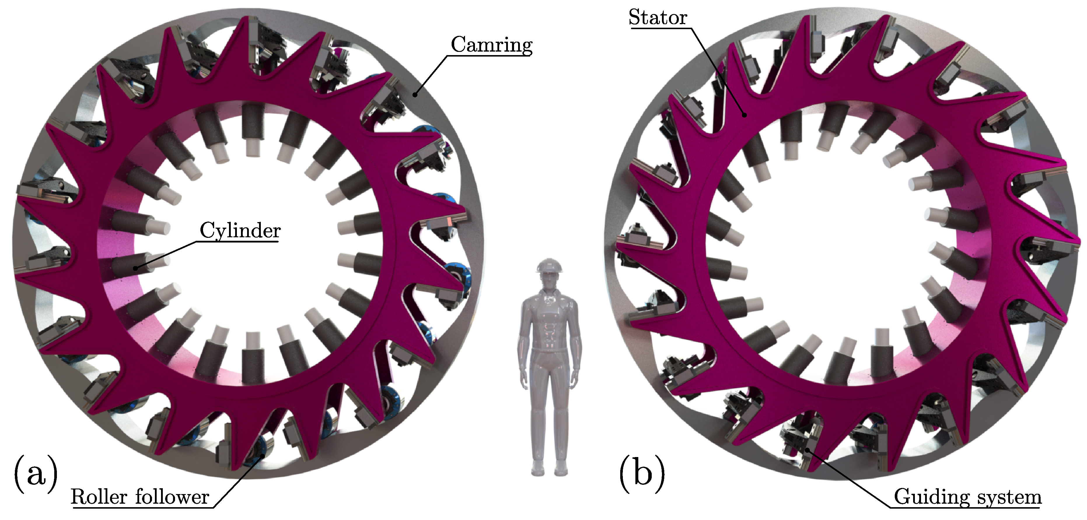
1.2. Cam-Roller Systems in Wind Turbines

In agreement with Nijssen et al. [4], the cam-follower unit is one of the most critical interfaces in a piston pump. A few publications can be found about hydraulic [5] and hydrostatic [6] drivetrains for wind turbines and also for tidal energy conversion [7]. In the latter as well as in [8] and Tao et al. [9], a low-speed multi-lobe camring pump forms part of the hydraulic transmission. However, the tribological performance of cam-roller interfaces is not discussed.

Cam-roller follower contacts operate under highly dynamic conditions. The lubricating film that separates the surfaces to avoid asperity contacts is critically affected by velocity and highly varying cyclic loads [10,11]. In fact, during one cycle, the curvature, the speed, the load, and even the surface roughness vary as a function of the cam angle. As a consequence, ensuring optimum lubrication of cam-roller contacts is a complex design task.

In the present case, the cam-roller contact and the SRBs are two coupled interdependent tribological systems. The internal spherical roller bearings (SRBs) (Figure 2) allow the roller to rotate on its axis, but also introduce a frictional torque. This means that the cam-roller contact and the SRBs are two coupled interdependent tribological systems. In other words, the frictional torque generated by the SRBs in combination with inertia effects results in a resisting torque acting on the roller, which can cause sliding at the cam-roller contact. The latter is often referred to in the literature as slippage and its level can be quantified with the slide-to-roll ratio ($SRR$).

The tribological behavior of cam-roller follower contacts has been studied mostly in valvetrain and diesel injection systems of internal combustion engines at smaller scales [11,12,13,14,15,16,17,18,19,20] but not in large-scale hydraulic drivetrains. Duffy [14] and others [16,17,18] have experimentally demonstrated the occurence of slippage in specialized setups. In a numerical study, Ji & Taylor [19] evaluated roller slippage in a simplified way by assuming a constant friction coefficient for the internal needle bearing. Only a few publications can be found where the possibility of slippage is considered in complex numerical lubrication models and its level is quantified by balancing the tractive and resisting torques acting on the roller [11,12,20]. From the studies above, it can be concluded that the occurrence of slippage is undesired and it remains a critical aspect also at smaller scales due to its potential to produce surface damage.

1.3. Offset Followers

The translation axis of the follower can be positioned in two ways: either aligned with the center of rotation of the cam, known as the radial follower configuration or with a specific eccentricity, known as the offset follower configuration (Figure 1). When downsizing, the latter can be utilized to modify the pressure angle and decrease the side thrust [21,22]. However, no comparative study of the rolling-sliding performance between radial and offset roller followers in large-scale hydraulic drivetrains has been conducted to date, to the best of our knowledge. Previous analyses assume zero eccentricity [13,23], and furthermore, the mechanisms investigated in these studies (e.g., [11,12,20]) are much smaller than those found in large-scale piston pumps, thus the significance of roller inertia is diminished.

In contrast to the conventional design of radial piston pumps featuring radial roller followers, this study proposes a novel approach by introducing offset roller followers. The primary objective is to minimize the “unnecessary” side thrust exerted on the guiding system, thereby significantly prolonging its operational lifespan. Moreover, we conduct a comprehensive analysis to compare the rolling-sliding performance between the traditional radial configuration and the innovative offset configuration. This investigation enables us to assess the potential drawbacks and advantages associated with the integration of offset followers in the pump design from a tribological point of view.

Our engineering framework offers a distinct advantage by eliminating the need for extensive simulations. This streamlined approach facilitates seamless integration into the design and optimization process of large-scale hydraulic drivetrains and it can be used to optimize eccentricity and provide a reasonable assessment of the tribological performance of cam-roller interfaces. In that way informed decisions to enhance the overall efficiency and reliability of large-scale hydraulic drivetrains can be made.

2. Mathematical Model

This section contains five different parts where the modeling approach is explained in detail. The kinematic and force analysis are presented in the first and second parts, respectively. Then, in part three, the torque balance equation is shown and the procedure to calculate slippage is described. In parts four and five, the lubrication models incorporated in the torque balance equation (to estimate traction and friction) are discussed. Figure 2 shows the configuration of the tribological system studied in this work. It consists of a multi-lobe camring (or ring cam), a roller follower, and two internal SRBs (with their inner ring fixed to a pin) that support the roller allowing it to rotate freely due to the traction force exerted by the cam. The lubricated interfaces considered in the analysis include the cam-roller contact and the SRBs. For simplicity, the former is assumed to be a (non-conformal) line contact.

The two-step computational process is summarized in Figure 3. First, the displacement profile $\sigma$ and a range of values for the eccentricity (i.e., offset) e is given to obtain the pressure angle ${\alpha }_c$ through the kinematic analysis. Then, the total force $F_T$ and the pressure angle ${\alpha }_c$ are used as input in the force analysis to find the minimum equivalent dynamic load $F_m$ and the optimum eccentricity e. In the second step, the displacement profile $\sigma$, the optimum e, and the total force $F_T$ are used as an input for the kinematic and force analysis to obtain the contact force $F_c$, the cam’s surface speed $U_c$, the pressure angle ${\alpha }_c$, the curvature of the cam ${\rho }_c$ and the roller velocity ${\omega }_c$ (under pure rolling conditions). These results are subsequently used as the input for the lubrication and frictional (L&F) analysis where the torque balance equation is iteratively solved to obtain the traction force $F_t$, the asperity load ratio $L_a$, the slide-to-roll ratio $SRR$, the surface temperature $T_s$, the heat dissipation rate $\dot{Q}$, the friction and traction coefficients ${\mu }_B$ and ${\mu }_{c-r}$, and the lambda ratio $\lambda$. For the comparison, the second step is also carried out for a radial follower configuration, where $e=0$.

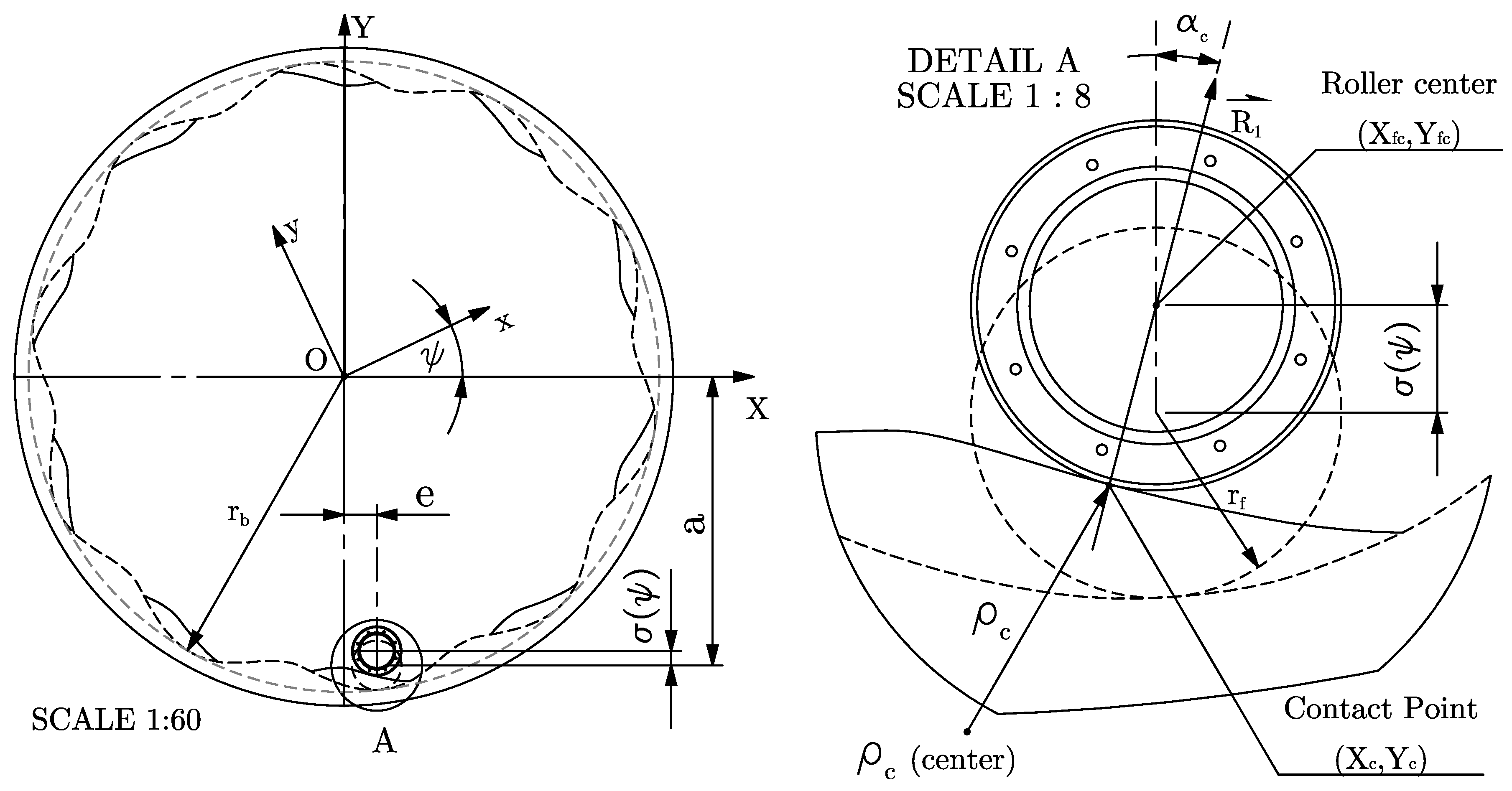
2.1. Kinematic Analysis

The kinematic analysis has been carried out as described by Matthews and Sadeghi [24] and adjusted for a translating follower and internal camring geometry. For more details, the reader is referred to their publication [24].

A schematic depicting different parameters considered for the kinematic analysis is shown in Figure 4. A global $(X,Y)$ and a relative $(x,y)$ coordinate system are used in the analysis, where the origin O of the global system, coincides with the center of the camring and it is fixed to the ground. The relative system is fixed to the camring and is used to derive the instantaneous radius of curvature ${\rho }_c$. The inputs required for the kinematic analysis include the displacement profile, $\sigma \left(\psi \right)$, as a function of the camring angle $\psi$, the roller follower radius $r_f$, the camring base radius $r_b$, the camring angular velocity ${\omega }_c$, and the global positions of the center of the roller $(X_{fc},Y_{fc})$ and contact point $(X_c,Y_c)$.The coordinates of the follower center in the $(X,Y)$ system are:

$$X_{fc}=e$$

(1)

$$Y_{fc}=\sigma \left(\psi \right)-a$$

(2)

where e is the eccentricity (i.e., offset) and a is a design-dependent parameter given by:

$$a=\sqrt{{(r_b-r_f)}^2-e^2}$$

(3)

The coordinates in the $(X,Y)$ can be transformed to the $(x,y)$ system, and vise versa, by using:

$$\left[\begin{array}{c}x\\ y\end{array}\right]=\left[\begin{array}{cc}cos\left(\psi \right)& sin\left(\psi \right)\\ -sin\left(\psi \right)& cos\left(\psi \right)\end{array}\right]\left[\begin{array}{c}X\\ Y\end{array}\right]$$

(4)

$$\left[\begin{array}{c}X\\ Y\end{array}\right]=\left[\begin{array}{cc}cos\left(\psi \right)& -sin\left(\psi \right)\\ sin\left(\psi \right)& cos\left(\psi \right)\end{array}\right]\left[\begin{array}{c}x\\ y\end{array}\right]$$

(5)

The instantaneous radius of curvature at the point of contact ${\rho }_c$ can be computed as follows:

$$\frac{{f_{fc}}^3}{f_{y_{fc}}{f}_{x_{fc}^{\prime }}-f_{x_{fc}}{f}_{y_{fc}^{\prime }}}+r_f$$

(6)

where

$$f_{fc}=\sqrt{{f_{x_{fc}}}^2+{f_{y_{fc}}}^2}$$

(7)

The first $f_{x_{fc}},f_{y_{fc}}$, and second $f_{x_{fc}}^{\prime },f_{y_{fc}}^{\prime }$, kinematic coefficients corresponding to the follower center are calculated as follows:

$$f_{x_{fc}}={\displaystyle \frac{\partial x_{fc}}{\partial \psi }}={\displaystyle \frac{\partial X_{fc}}{\partial \psi }}cos\left(\psi \right)-X_{fc}sin\left(\psi \right)+{\displaystyle \frac{\partial Y_{fc}}{\partial \psi }}sin\left(\psi \right)+Y_{fc}cos\left(\psi \right)$$

(8)

$$f_{y_{fc}}={\displaystyle \frac{\partial y_{fc}}{\partial \psi }}=-{\displaystyle \frac{\partial X_{fc}}{\partial \psi }}sin\left(\psi \right)-X_{fc}cos\left(\psi \right)+{\displaystyle \frac{\partial Y_{fc}}{\partial \psi }}cos\left(\psi \right)-Y_{fc}sin\left(\psi \right)$$

(9)

$$f_{x_{fc}}^{\prime }={\displaystyle \frac{{\partial }^2{x}_{fc}}{\partial {\psi }^2}}={\displaystyle \frac{{\partial }^2{X}_{fc}}{\partial {\psi }^2}}cos\left(\psi \right)+{\displaystyle \frac{{\partial }^2{Y}_{fc}}{\partial {\psi }^2}}sin\left(\psi \right)-2{\displaystyle \frac{\partial X_{fc}}{\partial \psi }}sin\left(\psi \right)+2{\displaystyle \frac{\partial Y_{fc}}{\partial \psi }}cos\left(\psi \right)-X_{fc}sin\left(\psi \right)-Y_{fc}cos\left(\psi \right)$$

(10)

$$f_{y_{fc}}^{\prime }={\displaystyle \frac{{\partial }^2{y}_{fc}}{\partial {\psi }^2}}=-{\displaystyle \frac{{\partial }^2{X}_{fc}}{\partial {\psi }^2}}sin\left(\psi \right)+{\displaystyle \frac{{\partial }^2{Y}_{fc}}{\partial {\psi }^2}}cos\left(\psi \right)-2{\displaystyle \frac{\partial X_{fc}}{\partial \psi }}cos\left(\psi \right)-2{\displaystyle \frac{\partial Y_{fc}}{\partial \psi }}sin\left(\psi \right)+X_{fc}sin\left(\psi \right)-Y_{fc}cos\left(\psi \right)$$

(11)

The coordinates of the contact point in the $(x,y)$ coordinate system are given by:

$$x_c=x_{fc}-r_f\frac{f_{y_{fc}}}{f_{fc}}$$

(12)

$$y_c=y_{fc}+r_f\frac{f_{x_{fc}}}{f_{fc}}$$

(13)

The coordinates $X_{fc},Y_{fc}$, and $X_c,Y_c$, are used to compute the direction of $\overrightarrow{R_1}$, ${\varphi }_1$. The vector $\overrightarrow{R_1}$, can be visualized as an imaginary link between the center of curvature of the cam and the center of the roller as depicted in Figure 4.

$${\varphi }_1=arctan\left(\frac{Y_{fc}-Y_c}{X_{fc}-X_c}\right)$$

(14)

Similarly, the pressure angle, ${\alpha }_c$, can be obtained as follows:

$${\alpha }_c=arctan\left(\frac{X_{fc}-X_c}{Y_{fc}-Y_c}\right)$$

(15)

The variation of the direction of the vector $\overrightarrow{R_1}$, $h_1$, is required for calculating the surface velocity of the camring $U_c$ and can be computed as follows:

$$h_1={\displaystyle \frac{\partial {\varphi }_1}{\partial \psi }}$$

(16)

The velocity of a point on the surface of the cam, $U_c$, relative to the point of contact, can be obtained with Equation (17) and the surface velocity of the roller, $U_r$, can be obtained with Equation (18), where ${\omega }_r$ is the angular velocity of the roller and thus, ${\dot{\omega }}_r$, the angular acceleration. The entrainment velocity of the lubricant $U_E$, is given by Equation (19).

$$U_c={\rho }_c{\omega }_c(1-h_1)$$

(17)

$$U_r=r_f({\omega }_r-{\omega }_c{h}_1)$$

(18)

$$U_E=\frac{U_c+U_r}{2}$$

(19)

In pure rolling conditions, $U_r$ can be assumed to be equal to $U_c$. However, to consider the possibility of sliding at the cam-roller interface, pure rolling cannot be assumed, since during slippage $U_c\ne U_r$. Hence, a different approach is required. The determination of the angular velocity of the roller allowing the possibility of slippage will be treated later on.

2.2. Force Analysis

Figure 1 shows the main components forming part of a large-scale hydraulic drivetrain. The stator remains fixed and it is used as a stiff structural support for cylinders and guiding systems. The torque generated by the wind is used to rotate the camring. When rotation starts, the roller followers convert the rotary motion of the camring into a translating motion to compress the water inside the cylinders. Figure 2a presentes a more detailed view of the principal components forming part of the cam-roller mechanism. The frame supports the pin, and two SRBs with their inner ring mounted on the pin support the roller allowing it to rotate in its axis. To displace the piston and transfer the resultant side thrust, the frame is connected to the guiding system and piston via two spherical joints. This configuration allows the roller to self-align and reduces edge loading at the cam-roller contact. The spherical joint 2 transfers the side thrust to the guiding system, while the roller runner blocks and rails allow the roller follower to translate. Note that the rails are fixed to the stator as shown in Figure 2b.

The forces acting on the cam-roller system are shown in Figure 2b, where $F_T$ is the total load, ${\tau }_t$ is the tractive torque, ${\tau }_B$ is the frictional torque from the SRBs, and ${\tau }_I$ is the inertia torque. The reaction force $R_x$ arises from the two roller runner blocks counteracting the side thrust in the positive and negative x-direction. For simplicity, the frictional forces generated by the guiding system are not considered in the analysis, since they are negligible when compared to the total force $F_T$. The tractive torque, ${\tau }_t$, is given by:

$${\tau }_t=F_t{r}_f=F_c{\mu }_{c-r}{r}_f$$

(20)

where $F_t$ is the traction force, $r_f$ the radius of the roller follower, $F_c$ the contact force, and ${\mu }_{c-r}$ the traction coefficient at the cam-roller contact. The components of $F_c$ and $F_t$ are given by:

$$F_{cx}=F_{c}sin\left({\alpha }_c\right)$$

(21)

$$F_{cy}=F_{c}cos\left({\alpha }_c\right)$$

(22)

$$F_{tx}=F_{t}cos\left({\alpha }_c\right)$$

(23)

$$F_{ty}=F_{t}sin\left({\alpha }_c\right)$$

(24)

The frictional torque from the spherical roller bearings, ${\tau }_B$, is given by:

$${\tau }_B=0.5F_c{\mu }_B{d}_m$$

(25)

where ${\mu }_B$ is the friction coefficient of the spherical roller bearings and $d_m$ is the mean bearing diameter. Note that the expression for ${\tau }_B$ accounts for the frictional torque produced by two internal roller spherical bearings. The inertia torque ${\tau }_I$ is given by:

$${\tau }_I=(I_r+2I_B){\dot{\omega }}_r=I_t{\dot{\omega }}_r$$

(26)

where $I_t$ is the total inertia and it accounts for the inertia of the roller, $I_r=0.5m_r(r_{fi}^2+r_f^2)$, and the inertia of the outer rings of two spherical roller bearings, $2I_B$, mounted on it. The inertia of the rest of the rotating bodies is rather small when compared to $I_t$. Hence, it has been neglected. From the analysis of forces, the contact force is given by:

$$F_c=\frac{F_T}{cos{\alpha }_c-{\mu }_{c-r}sin{\alpha }_c}$$

(27)

From Equation (27), it can be deduced that $F_c$ and $F_t$ are interrelated. The contact force affects the traction coefficient and vice-versa. Nevertheless, the contribution of $F_t$ to $F_c$ is very small, and therefore, $F_c$ can be considered independent [11,19]. Thus, the expression for $F_c$ is reduced to:

$$F_c=\frac{F_T}{cos{\alpha }_c}$$

(28)

The total load $F_T$ acting on the cam-roller pair of the piston pump (Figure 2) is obtained by adding up (from highest to lowest) the hydraulic force $F_h$, preload force $F_0$, inertia force $F_I$, and the weight of the follower unit $F_g$. For simplicity, the following realistic assumptions have been made:

• The follower unit is considered a single lumped mass.
• The rotational velocity of the camring is constant.
• The preload is constant
• The mass remains the same when eccentricity is introduced (i.e., when $e\ne 0$).

Therefore, $F_T$ can be computed as follows:

$$F_T=F_h+F_0+F_I+F_g$$

(29)

$$F_I=m_{eq}{\omega }_c^2{\displaystyle \frac{d^2\sigma }{d{\psi }^2}}$$

(30)

were the hydraulic force $F_h$ is given by the application and it is simply the product of the water pressure times the plunger area, $F_0$ is constant, and $F_g=m_{eq}g$, where g is the gravity and $m_{eq}$ is the equivalent lumped mass.

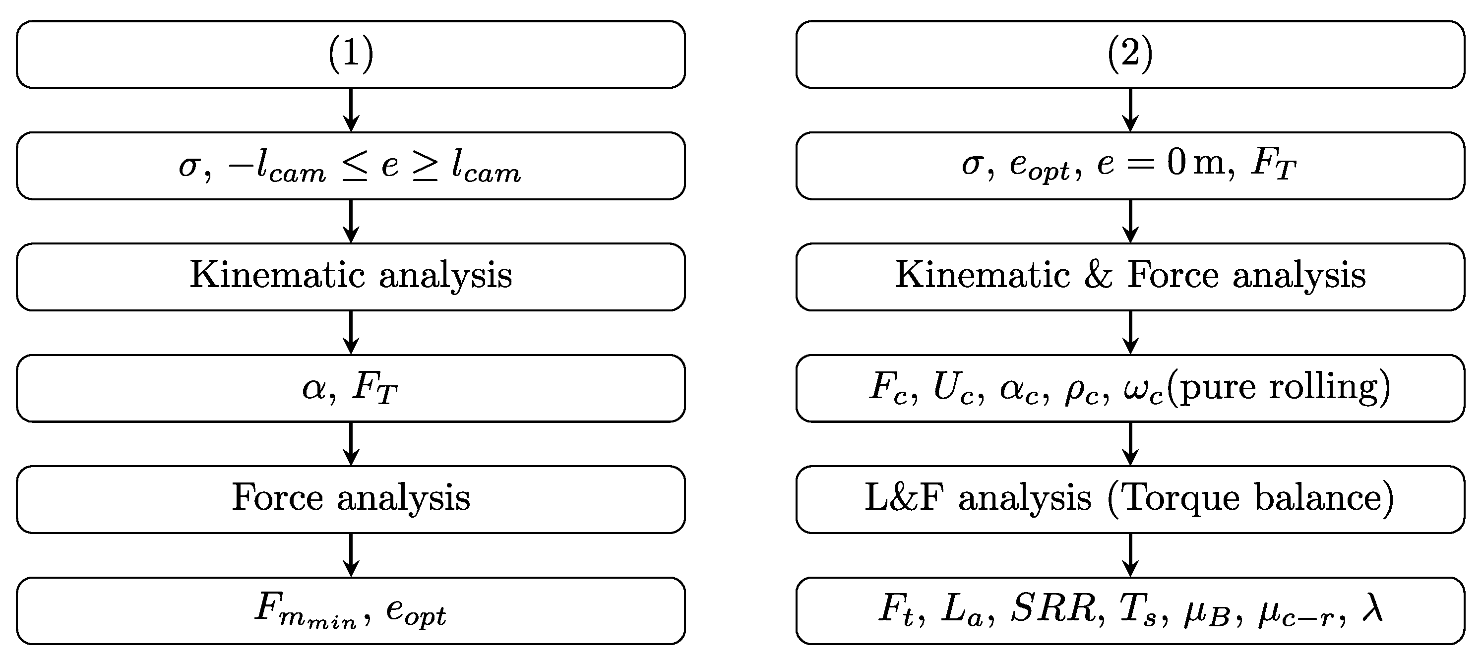
Follower Offset Optimization

In roller element bearings, the load is inversely proportional to lifetime, and hence, it is a critical factor in load-life calculations. For fluctuating loads, a dynamic equivalent load $F_m$ (a constant load that would have the same influence on fatigue life as the actual fluctuating load) is often used in the load-life calculations [25]. In this work, $F_m$ is selected as the objective function, where a minimum is sought to find the optimum offset (e). In that way, the lifetime of the roller runner blocks (Figure 2) counteracting the side thrust can be maximized. For the optimization, it has been assumed that the principal force in the x-direction is the side thrust $F_{cx}$, and that $F_{tx}$ and additional forces or moments are negligible. If preloading of the rolling elements is neglected, the dynamic equivalent load $F_m$ as a function of $\psi$, can be computed as follows [25]:

$$F_m^{10/3}=\frac{{\sum }_{j=1}^N\left|F_{c{x}_j}^{10/3}\right|}{{\psi }_{tot}}$$

(31)

$$F_{c{x}_{avg}}=\frac{{\sum }_{j=1}^N{F}_{c{x}_j}}{N}$$

(32)

where j is the counter for load phases, N is the number of load phases, ${\psi }_j$ is the individual cam angular displacement and ${\psi }_{tot}$ is the total angular displacement during one cam cycle, which includes the “rise” (during compression), and “fall” (during suction) (Figure 2) and it should not be confused with one revolution of the whole camring. Additionally, the average side thrust $F_{c{x}_{avg}}$, has been calculated with Equation (32) for the sake of comparison. The lower and upper limits chosen for e to find the minimum $F_m$ are $-l_{cam}$ and $l_{cam}$, where $l_{cam}=sin({\psi }_{tot}/2)r_b$.

2.3. Torque Balance

The torque balance equation (Equation (33)) has been used to predict roller slippage [11,12,20]. The tractive torque (on the LHS of the equation) drives the roller to make it roll on its axis whereas the frictional torque of the spherical roller bearings (on the RHS of the equation) resists the motion and tries to slow it down. Additionally, the roller is subjected to accelerations that result in the generation of inertia torques, which usually become more prominent at high speeds [14].

$${\tau }_t={\tau }_B+{\tau }_I$$

(33)

Speed changes can produce two different effects. When the roller’s angular velocity must increase due to the speed and tractive force exerted by the cam surface, positive acceleration is required. In this case, the rotational inertia will resist such acceleration potentially leading to positive slippage (i.e., the roller cannot catch up with the speed of the cam). In the second case, when the roller must slow down, “deceleration” (i.e., negative acceleration) is required. Under these conditions, the rotational inertia will resist deceleration and potentially result in negative slippage (i.e., the roller cannot slow down to match the speed of the cam).

$$F_c{\mu }_{c-r}{r}_f=0.5F_c{\mu }_B{d}_m+I_t{\dot{\omega }}_r$$

(34)

In Equation (34), ${\mu }_{c-r}$ and ${\mu }_B$ are unknown and they can be computed by using lubrication models. Their value depends strongly on the rotational speed of the roller ${\omega }_r$, which is also unknown if slippage occurs. To find a solution, ${\omega }_r$ is iteratively approximated until an established error criterion is satisfied. The speed of the roller ${\omega }_r$ is approximated at every condition in two stages. An initial guess for ${\omega }_r$ is given to start the iterative process. In the first stage, it is determined whether ${\omega }_r$ should increase or decrease to approach the solution, and fixed steps in ${\omega }_r$ are taken until two solutions bracketing the correct value are found. In the second stage, the step in ${\omega }_r$ is decreased by one order of magnitude to find two more accurate solutions bracketing the correct value. Stages one and two are repeated until a value for ${\omega }_r$ that satisfies the error criterion $|{\tau }_t-{\tau }_B-{\tau }_I|<1\times {10}^{-4} \mathrm{N}\mathrm{m}$ is found. The approximated speed of the roller ${\omega }_r$ for a previous condition is used as an initial guess for the next condition.

Including the kinematic analysis, a solution for a full camring profile (formed by 50,400 data points) can be obtained in approximately 32 $\mathrm{s}$ on a laptop Dell Precision 5560 with a processor Intel(R) Core(TM)i7-11850H. With regard to the accuracy, a comparison between the method employed for computing traction (i.e., ${\mu }_{c-r}$) and full TEHL simulations can be found in reference [26].

From Equation (33), it can be readily deduced that slippage occurs when the “required tractive torque” $({\tau }_B+{\tau }_I)$ on the RHS of the equation is higher than the “actual” tractive torque $\left({\tau }_t\right)$ on the LHS. This situation is likely to occur, for example, with high frictional torques produced by the SRBs, high acceleration caused by brusque variations of the cam’s surface speed, and/or loss of traction due to low contact forces. Furthermore, $I_t$ plays a critical role. With a limited amount of traction at the cam-roller interface, large inertias become much more difficult to drive. Hence the importance of optimizing mass and dimensions.

The required traction coefficient ${\mu }_{req}$ to achieve zero gross slip conditions can be easily obtained from Equation (35) assuming pure rolling and using the correspondent ${\omega }_r$, and ${\dot{\omega }}_r$ from the kinematic analysis. The required tractive torque is hence $F_c{\mu }_{req}{r}_f$. In the following sections, the lubrication models adopted to compute both, ${\mu }_{c-r}$ and ${\mu }_B$ will be described.

$${\mu }_{req}=\frac{0.5F_c{\mu }_B{d}_m+I_t{\dot{\omega }}_r}{F_c{r}_f}$$

(35)

2.4. Cam-Roller Traction

The prediction of traction is essential in multiple engineering applications. Shirzadegan et al. [27] and Masjedi & Khonsari [26] presented rapid approaches for estimating traction in EHL and mixed–EHL contacts, respectively. In this work, the latter has been adopted to account for the asperity friction component in case contact occurs. A detailed description can be found in references [26,28,29]. The most relevant details about the model and equations are presented in the Appendix A. According to [26], the traction coefficient ${\mu }_{c-r}$ can be obtained as follows:

$${\mu }_{c-r}=\frac{F_t}{F_c}=\left(\frac{L_a}{100}\right)f_c+\frac{2bB{\tau }_{lim}}{F_c}\left[1-exp\frac{-{\eta }_{avg}{u}_s}{{\tau }_{lim}{h}_c}\right]$$

(36)

2.5. Spherical Roller Bearings Friction

As mentioned before, in some previous studies [13,19], the friction coefficient of the rolling element bearing inside the roller has been considered constant. Nevertheless, in reality, bearing friction varies with speed and load [30]. In this work, the SKF model has been used to approximate the bearing frictional torque. A detailed description of the method can be found in [30]. The most relevant details are given in the Appendix B. With $F_c$ (in $\mathrm{N}$), and the mean bearing diameter $d_m$ (in $\mathrm{m}\mathrm{m}$), the SRB friction coefficient can be computed as follows:

$${\mu }_B=\frac{4\times {10}^3{\tau }_{SRB}}{F_c{d}_m}$$

(37)

where ${\tau }_{SRB}$ is the frictional torque produced by one SRB.

3. Results and Discussion

For clarity, Section 3 has been divided into four subsections. Section 3.1 introduces the displacement $\sigma$ and total load $F_T$ profiles used throughout the two-step computational process (Figure 3), which remain unchanged during the analysis. Section 3.2 shows the results of the optimization, where $\sigma$ and $F_T$ have been used to find the optimum offset e that yields the minimum $F_m$. Section 3.3 presents the differences in the roller’s angular speed ${\omega }_r$ and cam surface velocity $U_c$ for the radial follower (RF) configuration and the offset follower (OF) configuration (with optimum e). Finally, Section 3.4 presents and compares the results of the lubrication and frictional analysis for the two aforementioned configurations.

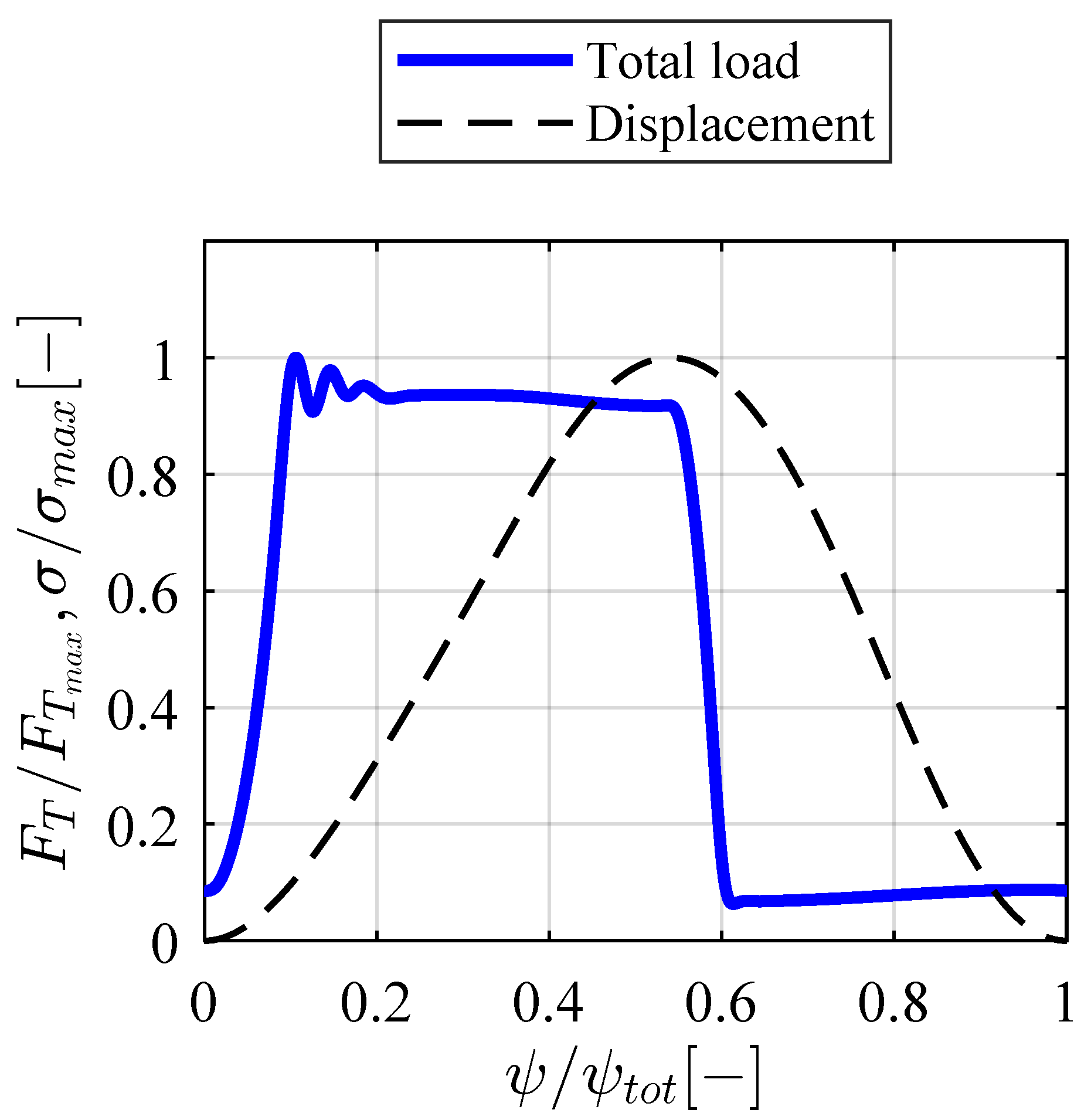
3.1. Displacement and Total Load Profiles

Figure 5 shows the displacement profile $\sigma$ and total load profile $F_T$ (in normalized form) used as input for this work. The displacement profile $\sigma$ was derived through a two-step optimization process. In the first step, efficiency was maximized and the mass of components was minimized by finding the optimum pump and geometry parameters. In the second step, the displacement profile $\sigma$ was adjusted to optimize the mechanical and hydraulic stability of the system. In both steps, the optimum combination of design-dependent variables was found by making use of gradient-free algorithms. More details about the optimization process are not further discussed in this work

The total load profile $F_T$ is obtained by adding up $F_h+F_0+F_I+F_g$ as explained in Section 2.2. The shape of the force profile mainly reflects the pressure profile, since hydraulic forces contribute the most to the total load. The load profile is highly asymmetric (with respect to the displacement profile) and contains abrupt variations. The high-load phase corresponds to the compression stroke and the low-load phase to the suction stroke. The oscillations that follow the peak load reflect the pressure overshoot produced by the discharge valve lag [31]. After the sudden load decrease at the end of the compression stroke, the small oscillation corresponds to the underpressure spike due to the lag of the suction valve [31].

The pressure profile has been modeled from experimental data obtained through extensive testing on a full-scale setup. During the tests, the evolution of the water pressure inside the cylinder chamber with respect to time has been investigated under a wide range of operating conditions within the pump’s operating envelope. The experimental data has been used as a baseline to model the evolution of the cylinder pressure over the cam, as it provides information on the magnitude and location of pressure spikes as well as on the duration of the transitions between suction and compression stroke. The simplified pressure profile includes fundamental characteristics observed in the overpressure, underpressure, and transition regions, whereas constant pressure is assumed for the suction and compression sections between transient behavior. Further details on the pressure profile will not be presented here.

3.2. Follower Offset Optimization Results

The geometrical parameters and reference conditions for the kinematic and force analysis can be found in

Table 1. Geometrical parameters and reference conditions for the kinematic and force analysis.

Parameter	Value	Unit
$F_g$	2	$\mathrm{k}\mathrm{N}$
$F_0$	33	$\mathrm{k}\mathrm{N}$
$l_{cam}$	0.592	$\mathrm{m}$
$m_{eq}$	204	$\mathrm{k}\mathrm{g}$
$r_b$	1.91	$\mathrm{m}$
$r_f$	0.150	$\mathrm{m}$
${\omega }_c$	1.6	$\mathrm{rad} {\mathrm{s}}^{-1}$

and the results of the follower offset optimization are presented in Figure 6, where e was varied from $-l_{cam}$ to $l_{cam}$ to compute $F_m$ and $F_{c{x}_{avg}}$. For a radial follower (RF), $e/l_{cam}=0$. For this configuration, neither $F_m$ nor $F_{c{x}_{avg}}$ are the lowest.

Negative offset values increase the side thrust, whereas positive offset values lead to a significant reduction of both, the dynamic equivalent load and average side thrust. For the given displacement and load profiles (Figure 5), the lowest $F_m$ can be attained with an offset follower (OF) configuration at $e/l_{cam}=0.635$, which corresponds to $e=0.375 \mathrm{m}$. This means that the lifetime of the guiding system shown in Figure 2 could be greatly increased by incorporating offset roller followers positioned at a distance $e=0.375 \mathrm{m}$ with respect to the center of the camring.

It is interesting to point out that the minimum $F_{c{x}_{avg}}$ occurs with a slightly higher amount of offset, namely $e/l_{cam}=0.83$. Therefore, minimizing $F_m$, by introducing eccentricity does not necessarily yield the lowest average side thrust too. This suggests that different results might be expected if, for example, the optimum offset value that minimizes friction losses in the guiding system is sought.

Figure 7 shows the pressure angle ${\alpha }_c$ (in $°$) and the normalized contact force $F_c$ for the RF and OF configurations. It is important to acknowledge that the displacement profile is non-symmetrical, and thus, the absolute pressure angle values during compression and suction strokes are not the same. This intentional asymmetry aims to moderate the pressure angle ${\alpha }_c$ during compression to control the magnitude of the side thrust. For the RF configuration, the maximum $|{\alpha }_c|$ during the compression and suction strokes are $20.6$$°$ and $26.3$$°$, respectively. On the other hand, by optimizing e, the maximum $|{\alpha }_c|$ can be reduced to $8.8$$°$ during the compression stroke and increased to $36.2$$°$ during the suction stroke. This notable reduction in the pressure angle attained with the OF configuration (during the compression stroke) enables a significant side thrust reduction (Figure 8), particularly where the total load $F_T$ is high. Additionally, it should be noted that the OF configuration brings positive changes to the contact force $F_c$ when compared to the RF configuration. During the compression stroke, $F_c$ is slightly reduced (lowering contact stresses) and during suction, it is slightly increased (enhancing traction).

Figure 8 shows the side thrust profile ($F_{cx}$) and the correspondent equivalent dynamic load $F_m$ for the RF and OF configurations. In the RF configuration, the side thrust yields an equivalent dynamic load $F_m=101.7 \mathrm{kN}$, with $|F_{cx}|$ rising above 153 $\mathrm{k}$$\mathrm{N}$ during the compression stroke. In the RF configuration, a notable characteristic is that at maximum displacement, ${\alpha }_c=0°$ (Figure 7), resulting in $|F_{cx}|=0 \mathrm{k}\mathrm{N}$. In addition, during the compression stroke, the side thrust remains positive and transitions to negative in the suction stroke.

In contrast, with optimum e, the side thrust yields an equivalent dynamic load $F_m=50.2 \mathrm{k}\mathrm{N}$, meaning that the OF configuration (Figure 1) enables a 51% reduction in the equivalent dynamic load $F_m$. Additionally, the maximum $|F_{cx}|$ drops substantially to 107 $\mathrm{k}$$\mathrm{N}$. Unlike the RF configuration $|F_{cx}|$ reaches its maximum at maximum displacement, where ${\alpha }_c\ne 0°$. Regarding sign changes, the side thrust displays both, negative and positive values during the compression stroke, and only negative values during the suction stroke. The conceptual design of the conventional “radial piston pump” (RPP) and the proposed “offset piston pump” (OPP) can be seen in Figure 1.

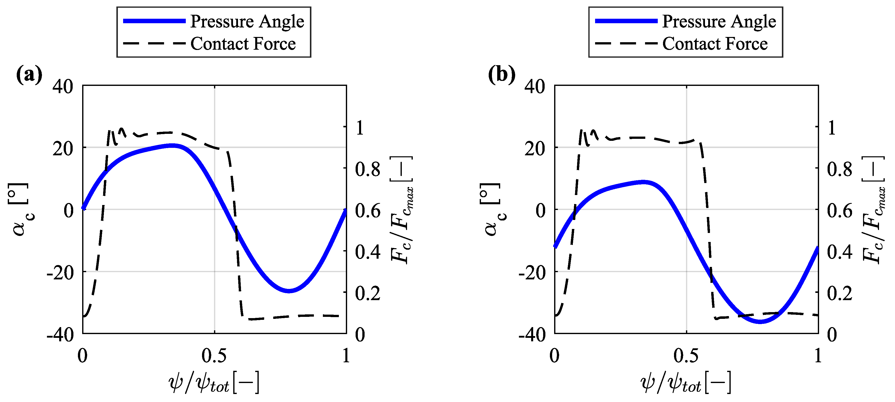
3.3. Kinematics

Figure 9 shows the cam surface velocities $U_c$ and roller angular velocities ${\omega }_r$ for the RF and OF configurations (computed assuming pure rolling). From Equations (1) and (2), it becomes evident that introducing offset, (i.e., $e\ne 0\mathrm{m}$) changes the global position of the center of the roller follower, and hence, the relative position in the $(x,y)$ coordinate system. Consequently, changes in the camring curvature, surface velocity, pressure angle, and the side thrust magnitude must be expected, even while the displacement profile $\sigma \left(\psi \right)$ is maintained. In this case, the optimum eccentricity ($e=0.375\mathrm{m}$), results in a slight reduction of the cam’s surface speed during the compression stroke and a slight increase during suction. The effects of eccentricity are much more evident in the roller’s angular speed, where ${\omega }_r$ decreases during compression and increases during suction. The differences between the velocities of both configurations are attributed to the changes in the curvature of the cam ${\rho }_c$ and the movement of the point of contact (i.e., $h_1$).

In addition, in Figure 9, it is also important to note that the entrainment motion (i.e., $U_c$) remains above zero. Hence, for the calculation of film thickness, squeezing motion can be neglected [32]. In situations where flow reversal does not occur, transient effects appear to be negligible in the prediction of changes in the oil film thickness [10,11]. Therefore, in this work, the quasi-static solution has been considered suitable and valuable for predicting the tribological behavior of the cam-roller contact.

3.4. Lubrication and Frictional Analysis

The cam-roller and the SRBs are grease-lubricated interfaces. For the former, a calcium sulphonate grease with mineral base oil (CaSMi) has been selected and it is assumed that its properties are equal to that of its base oil. This assumption remains valid for CaSMi at entrainment speeds above $0.2$ $\mathrm{m}$/$\mathrm{s}$⁻¹. This means that standard EHL theories can be used to predict film thickness and traction provided there is sufficient entrainment speed [33].

Table 2. Cam-roller contact reference conditions.

Parameter	Value	Unit
B	0.150	$\mathrm{m}$
$C_p$	450	$\mathrm{J} \mathrm{k}{\mathrm{g}}^{-1}{\mathrm{K}}^{-1}$
E	210	$\mathrm{G}\mathrm{Pa}$
$E^{\prime }$	231	$\mathrm{G}\mathrm{Pa}$
$I_r$	0.70	$\mathrm{k}\mathrm{g} {\mathrm{m}}^2$
$I_t$	0.76	$\mathrm{k}\mathrm{g} {\mathrm{m}}^2$
k	21	$\mathrm{W} {\mathrm{m}}^{-\mathrm{l}}{\mathrm{K}}^{-\mathrm{l}}$
$l_r$	0.165	$\mathrm{m}$
$m_r$	39.8	$\mathrm{k}\mathrm{g}$
$r_{fi}$	0.1125	$\mathrm{m}$
$R_q$	0.8	$\mathrm{\mu m}$
$T_{c-r}$	50	$°\mathrm{C}$
v	6.87	$\mathrm{G}\mathrm{Pa}$
Z	0.48	−
$\alpha$	19.6	$\mathrm{G}{\mathrm{Pa}}^{-1}$
$\beta$	0.0472	−
${\eta }_0$	192.2	$\mathrm{m}\mathrm{Pa}\mathrm{s}$
${\eta }_{40}$	367.7	$\mathrm{m}\mathrm{Pa}\mathrm{s}$
${\eta }_{100}$	20.7	$\mathrm{m}\mathrm{Pa}\mathrm{s}$
${\lambda }_{lim}$	0.0485	−
$\nu$	0.3	−
$\rho$	7800	$\mathrm{k}\mathrm{g} {\mathrm{m}}^{-3}$
${\sigma }_q$	1.13	μ $\mathrm{m}$

shows the reference conditions for the lubrication and frictional analysis of the cam-roller contact. The viscosity of the paraffinic/naphthenic mixture base oil is provided by the supplier. The dynamic viscosity has been calculated by assuming ${\rho }_{lub}=869 \mathrm{k}\mathrm{g}/{\mathrm{m}}^3$. The inlet viscosity (at the operating temperature), has been calculated according to the ASTM standard [34]. The limiting shear stress and the pressure viscosity coefficients have been interpolated from the tables presented in [35] for the above-mentioned mixture. The asperity friction coefficient, $f_c$ has been assumed to be 0.12.

The cam and the roller follower are made of high-strength low-alloy steel. The assumed values in Table 2 for the specific heat $c_p$, thermal conductivity k, density $\rho$, elastic modulus E, and Poisson’s ratio $\nu$ apply for both, the cam and the roller follower. The thermal conductivity value (i.e., $k=21 \mathrm{W}{\mathrm{m}}^{-1}{\mathrm{K}}^{-1}$) corresponds to hardened steels [36] to prevent overestimating traction in the EHL regime [37,38].

Table 3. SRBs reference conditions.

Parameter	Value	Unit
D	225	$\mathrm{m}\mathrm{m}$
d	150	$\mathrm{m}\mathrm{m}$
$d_m$	187.5	$\mathrm{m}\mathrm{m}$
$I_B$	0.03	$\mathrm{k}\mathrm{g} {\mathrm{m}}^2$
$T_{SRB}$	55	$°\mathrm{C}$
${\mu }_{bl}$	0.12	−
${\nu }_{SRB}$	87.3	$\mathrm{m}\mathrm{m} {\mathrm{s}}^{-2}$

contains the reference conditions for the SRBs. Note that the type of grease and operating temperature are different from that of the cam-roller contact.

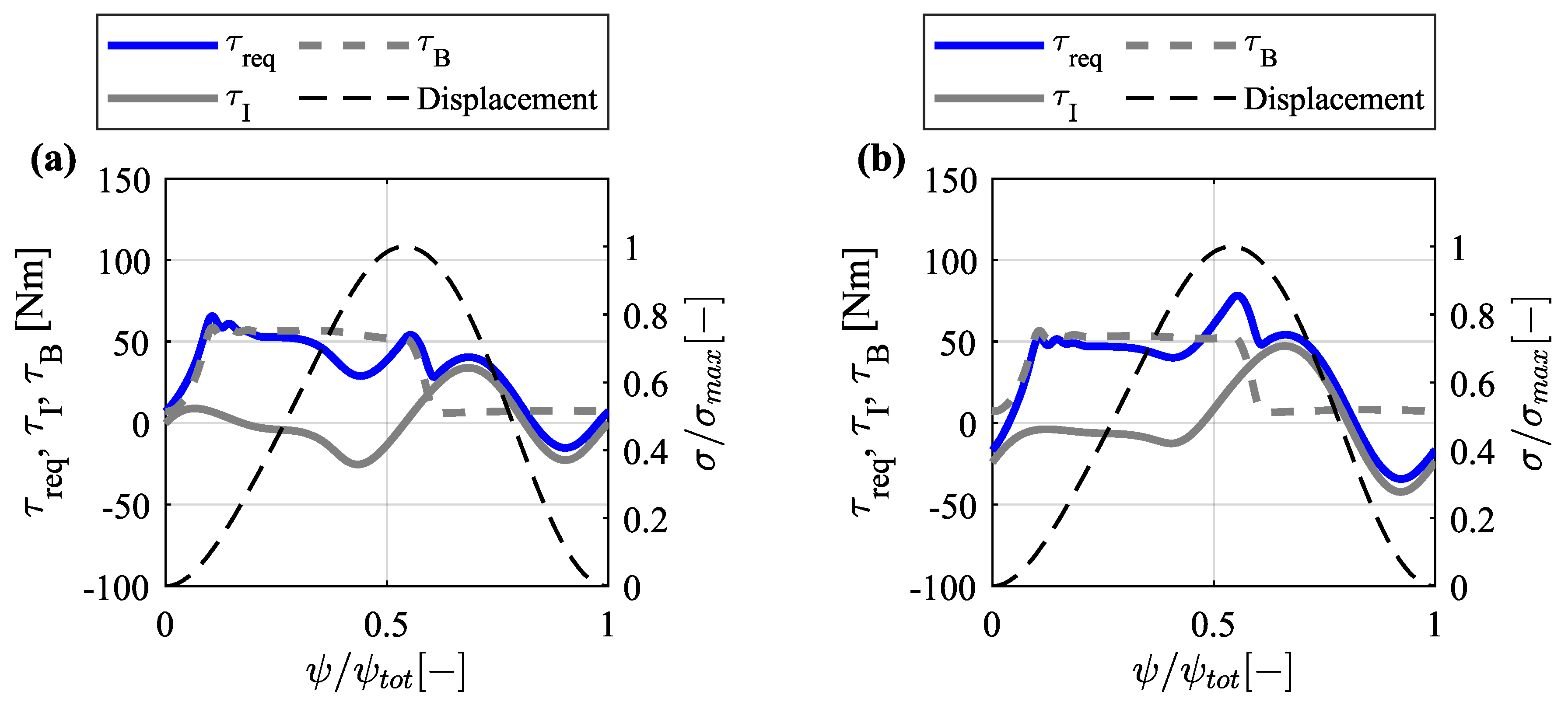
3.4.1. Required Tractive Torque

Figure 10 illustrates the computation of various torques: the frictional torque ${\tau }_B$ determined by the SKF model, the inertia torque ${\tau }_I$, and the required tractive torque, represented as ${\tau }_B+{\tau }_I$. The required tractive torque to avoid gross sliding can be easily obtained using Equation (35) as explained earlier. It is important to note that the required tractive torque differs between the RF and OF configurations due to changes in ${\omega }_r$ and ${\dot{\omega }}_r$. The most notable difference is the higher ${\tau }_I$ peaks for the OF configuration that occur as a result of increased angular accelerations. However, in regard to the frictional torque ${\tau }_B$, the differences are minimal. Both configurations exhibit a noteworthy outcome when negative inertia torques arise. Under such conditions, the friction generated by the SRBs aids in deceleration, effectively acting as a braking mechanism, and thereby reducing the tractive torque required to slow down the roller.

The SKF model provides a fast and reasonable estimation of the frictional torque, but it is mostly suitable for steady conditions. Therefore, complex dynamic effects produced by load and speed changes that could affect the frictional torque might not be entirely captured with this approach. For dynamic simulation of lubricated roller bearings, highly complex and computationally expensive methods are required [39].

3.4.2. Lubrication Regime

Figure 11 shows the lambda ratio $\lambda$ and the load asperity ratio $L_a$ for the RF and OF configurations. These results have been obtained taking roller slippage into account. Only small differences can be observed between the two configurations.

In both cases, the lubrication regime is dependent to a great extent on the entrainment speed, and to a lesser extent on the load. The reduction in the film parameter to $\lambda \approx 2$ indicates that mixed-EHL occurs around the nose of the cam. This change in the lubrication regime can be attributed to the decreasing entrainment speed and increasing curvature. The latter is also responsible for the rise in the maximum contact pressure that can be observed in Figure 12 at maximum displacement. Additionally, in this region, the asperity load ratio reaches values between 4 to $4.5$%, indicating that asperity contact occurs. With increasing entrainment velocities, the film parameter grows to $\lambda \ge 3$, while $L_a$ drops to levels close to zero indicating that EHL is attained as the roller approaches the cam’s base circle.

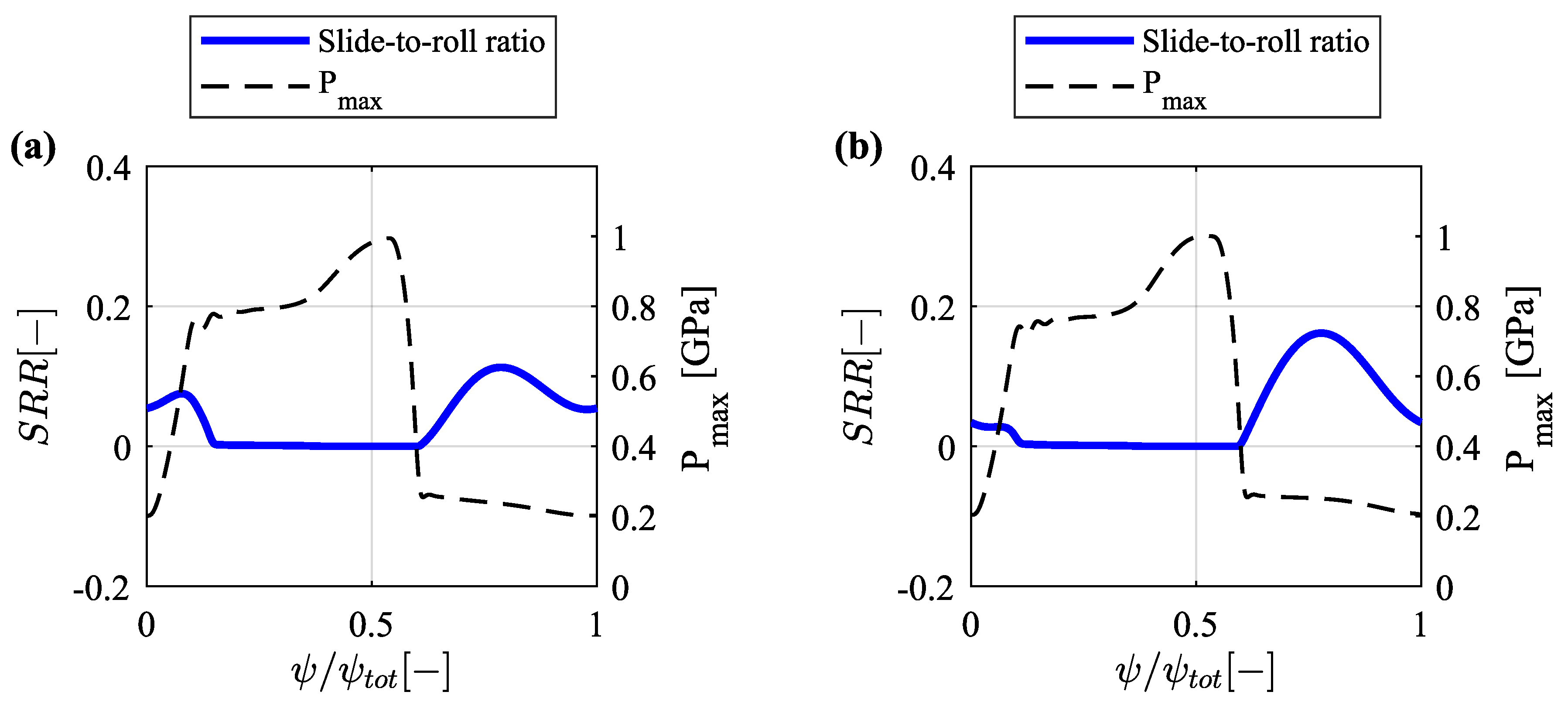
3.4.3. Roller Slippage

Figure 12 shows the $SRR$ predictions and the maximum contact pressure ($P_{max}$) profiles for the RF and OF configurations. Similar to the total load profile (Figure 5), the contact pressure along the cam is also highly varying, ranging from approximately 0.2 to 1 $\mathrm{G}$$\mathrm{Pa}$. For both configurations, relatively high slip ratios are predicted during the low-load phase, where the contact pressure drops substantially.

At low contact pressures, the maximum $SRR$ is 11.3% and 16.2% for the RF and OF configurations, respectively. At the end of the suction phase ($\psi /{\psi }_{tot}=1$) (i.e., the beginning of the compression phase), the $SRR$ is 5.4% and 3.3% for the RF and OF configurations, respectively. This means that for both configurations, the roller enters the compression phase with some degree of slippage. Figure 12 shows that between $\psi /{\psi }_{tot}=0$ and $\psi /{\psi }_{tot}=0.15$, slippage occurs in combination with high contact pressures, and thus, the operating conditions can be regarded as critical. Nevertheless, due to the drastic increase in contact pressure, the predictions show a brusque change in the rolling condition, where the $SRR$ rapidly drops to practically zero. Here, it is important to mention that in regions where asperity contact takes place, $SRR$ levels slightly above zero could be anticipated, since the employed approach may slightly overestimate traction when asperity contact is involved [40].

Two key differences must be highlighted between the RF and OF configurations. With an offset roller follower, more slip is predicted at low contact pressures and less slip during the contact pressure rise. The opposite holds for the RF configuration. The generation of higher slip levels in the OF configuration can be attributed to the higher required tractive torque Figure 10 (i.e., more slippage is required during torque balancing to satisfy the expression). The reduction of slip at the beginning of the high-load phase can be attributed to the angular speed of the roller. In the OF configuration, during the suction stroke, the roller experiences higher accelerations, which right before entering the high-load phase, bring ${\omega }_r$ closer to the roller’s speed in pure rolling conditions.

Duffy [14] measured slippage during high accelerations and low contact forces and suggested that under these conditions slippage is “benign”, but it becomes critical if it occurs in combination with high contact forces. Furthermore, previous studies have demonstrated that brusque changes in the rolling condition can potentially cause smearing on the surfaces [41,42]. In regard to the lubricant, shearing and heating, can lead to a nonuniform flow of grease eventually causing the breakdown of the lubricating film and potentially wear [43]. Besides, the lubrication of the internal SRBs is highly dependent on the rotational speed of the roller, and thus, it could also be affected if excessive slippage occurs.

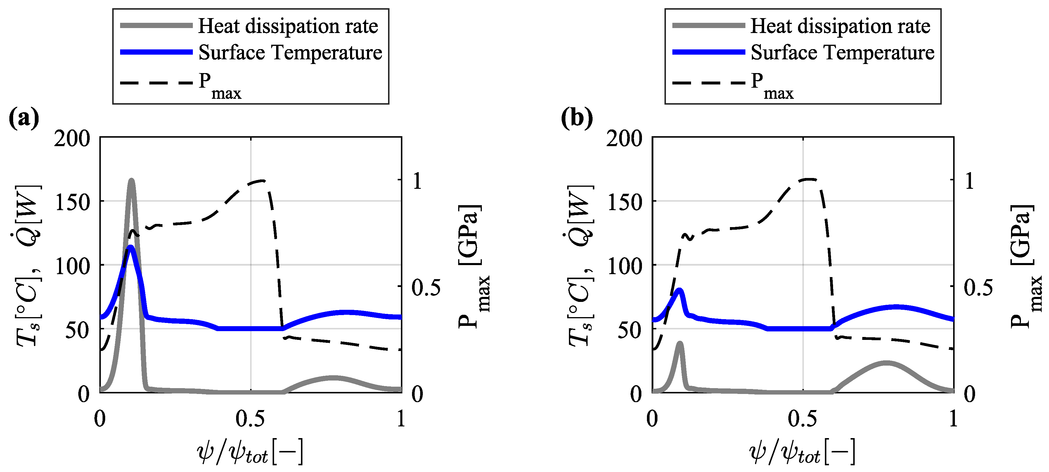
3.4.4. Surface Temperature

Figure 13 shows the heat dissipation rate $\dot{Q}=F_c{u}_s{F}_t$ [36] and the surface temperature $T_s$ computed as described in reference [26]. For the conditions and slip levels observed (i.e., $SRR<0.16$), the temperature rise may well still be close to that predicted by full TEHL solutions, since deviations occur particularly at high loads and higher slide-to-roll ratios.

The sharp increase in the heat dissipation rate $\dot{Q}$ and surface temperature $T_s$ taking place between $\psi /{\psi }_{tot}=0$ and $\psi /{\psi }_{tot}=0.15$, can be attributed to the occurrence of slippage in combination with high contact forces (Figure 12). At higher temperatures, the average viscosity ${\mu }_{avg}$ drops causing a reduction in the traction coefficient ${\mu }_{c-r}$ at a given $SRR$. As a result, more slippage is required to balance Equation (33).

For the RF configuration, the peak heat dissipation rate $\dot{Q}$ and surface temperature $T_s$ values are 166 W and 114 $°$C, respectively, whereas for the OF configuration, these peaks are substantially lessened to $\dot{Q}=39\mathrm{W}$ and $T_s$ = 80 $°$C.

As the contact pressure increases, traction improves, slip vanishes, and hence, heat and temperature drop. When the contact pressure falls, a smaller rise in the heat dissipation rate $\dot{Q}$ and surface temperature $T_s$ is predicted, due to the occurrence of slippage in combination with low contact forces.

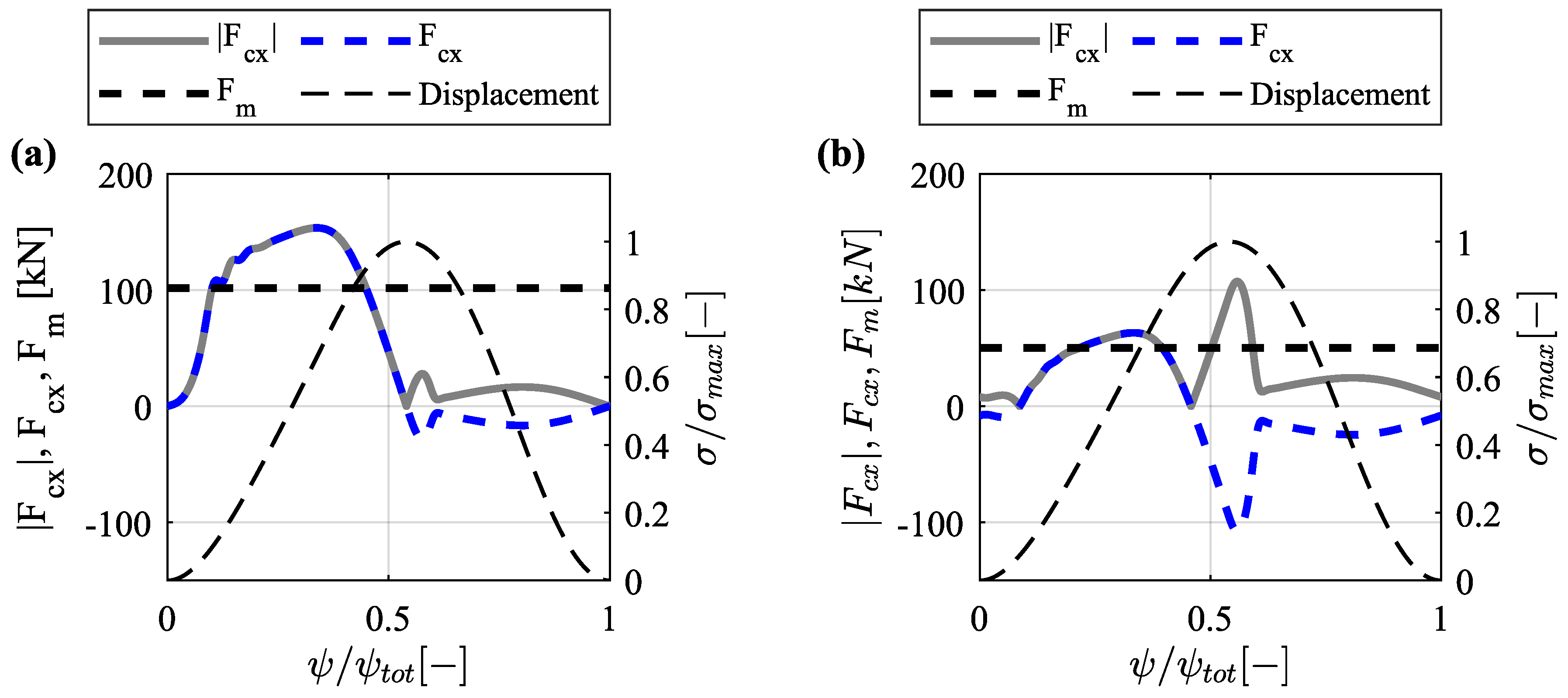
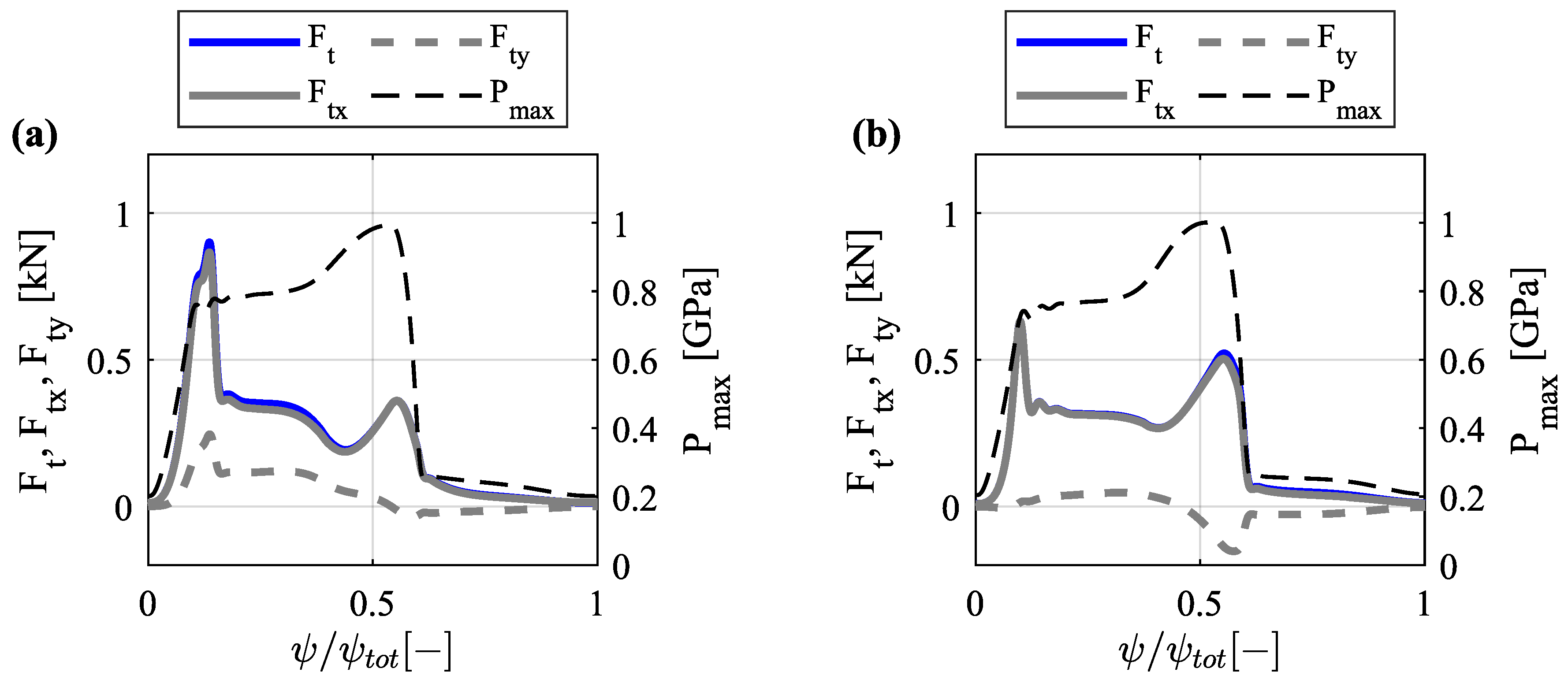
3.4.5. Traction Force

Minimizing slippage in the studied cam-roller system proves to be vital not only to prevent wear, improve lubrication and reduce heat generation but also to reduce impact loads. This becomes evident by looking at Figure 14, where the traction force and its components are shown. It is interesting to see, that for the RF configuration, the traction force reaches a peak value of $0.9 \mathrm{k}\mathrm{N}$ at the beginning of the compression stroke, between $\psi /{\psi }_{tot}=0$ and $\psi /{\psi }_{tot}=0.15$. This occurs as the roller enters the highly-loaded region with relatively high slip levels. In other words, with high loads, the sliding roller is forced to catch up with the cam’s surface speed in a brusque fashion giving rise to sharp peaks in the acceleration and inertia torque and provoking the traction force spike observed in the graphs. This behavior is comparable to that of rolling elements in large-scale bearings during the unloaded-loaded transition, where the conditions are favorable for smearing to occur [42,44]. For the OF configuration, the traction force peak value is reduced to $0.6 \mathrm{k}\mathrm{N}$, since smaller slip levels are predicted at the beginning of the compression stroke. These results highlight the importance of minimizing slippage.

4. Conclusions

In this study, the integration of offset followers in large-scale hydraulic drivetrains to mitigate the equivalent side thrust and enhance the lifespan of the guiding systems has been proposed. Moreover, a comprehensive comparison between the conventional radial roller follower and the innovative offset roller follower configuration has been carried out in terms of rolling-sliding performance. This investigation enables the assessment of the potential drawbacks and advantages associated with the integration of offset followers in the pump design from a tribological point of view.

• The follower offset optimization results show that for the given displacement profile $\sigma$ and total load profile $F_T$, the equivalent dynamic load $F_m$ counteracted by the guiding system can be reduced by $51\%$ from $F_m=101.7 \mathrm{kN}$ to $F_m=50.2 \mathrm{k}\mathrm{N}$, by incorporating offset roller followers at a distance $e=0.375 \mathrm{m}$ with respect to the center of the camring. By minimizing $F_m$, the lifetime of the guiding systems can be substantially improved.
• The kinematic analysis shows that while maintaining the optimum displacement profile $\sigma$ unchanged, the curvature ${\rho }_c$ of the cam, and hence, its surface speed $U_c$ change when offset roller followers are incorporated. These kinematic changes have a significant influence on the rolling-sliding behavior of the roller followers.
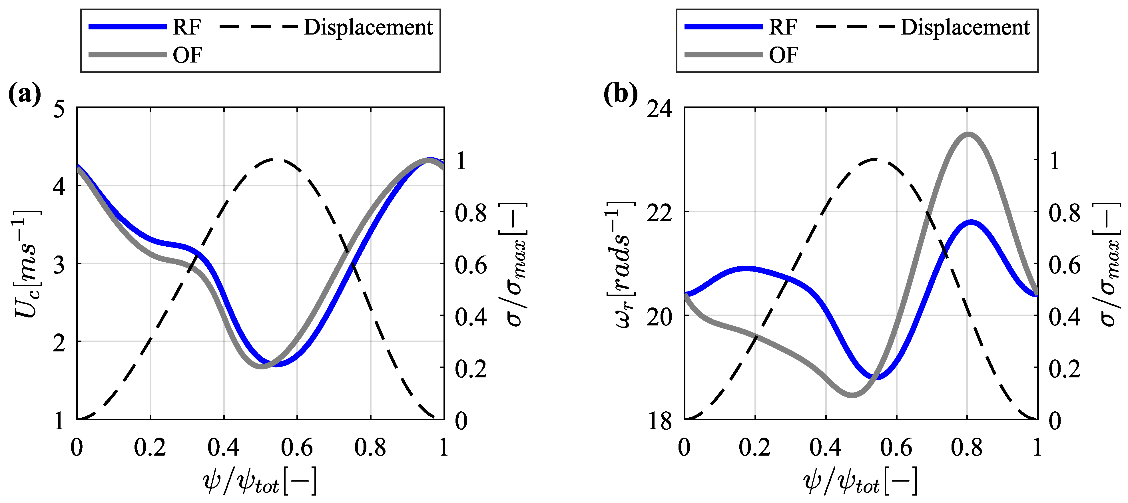
• The lubricating regime in the studied cam-roller contact is primarily influenced by the entrainment speed and to a lesser extent by the load. Both the radial roller follower (RF) and the offset roller follower (OF) configurations show similar behavior, with mixed-EHL ($\lambda \approx 2$ and $L_a\approx 4\%$) occurring around the cam’s nose due to decreasing entrainment speed and increasing curvature. The latter is also responsible for the increase in the maximum contact pressure (to $1 \mathrm{G}\mathrm{Pa}$) at maximum displacement.
• For the RF and OF configurations, the results of the lubrication and frictional analysis predict relatively high slide-to-roll ratios during low contact pressures and a rapid transition to virtually pure rolling at high contact pressures. At low contact pressures, the maximum $SRR$ is $11.3\%$ and $16.2\%$, for the RF and OF configuration, respectively. However, at the beginning of the compression phase, where the contact force and contact pressure increase, the OF configuration displays lower $SRR$ levels (3.3%) compared to the RF configuration ($SRR=5.4\%$). The occurrence of slippage in combination with high contact forces is considered critical, due to its potential to cause surface damage. From the analysis, the operating conditions generated between $\psi /{\psi }_{tot}=0$ and $\psi /{\psi }_{tot}=0.15$ have been regarded as critical, since slippage leads to sharp increases in the surface temperature, heat dissipation rate, and traction force at the cam-roller interface. Remarkably, offset roller followers show superior tribological performance which leads to improved rolling-sliding behavior. With less slippage occurring between $\psi /{\psi }_{tot}=0$ and $\psi /{\psi }_{tot}=0.15$, the peak heat dissipation rate drops substantially from $\dot{Q}=166\mathrm{W}$ to $\dot{Q}=39\mathrm{W}$, the peak surface temperature decreases from $T_s$ = 114 $°$C to $T_s$ = 80 $°$C and the peak traction force drops from $0.9 \mathrm{k}\mathrm{N}$ to $0.6 \mathrm{k}\mathrm{N}$.

In conclusion, the incorporation of offset followers in unidirectional piston pumps with highly varying loading conditions offers significant benefits. By introducing roller eccentricity, the equivalent side thrust can be substantially reduced, leading to a notable extension of the guiding system’s lifespan. Moreover, for the reference conditions assumed in this study, the integration of offset followers results in improved rolling-sliding behavior and enhanced tribological performance, which leads to the attenuation of unfavorable thermal and dynamic effects.

The developed framework presents a notable advantage by eliminating the need for extensive simulations. Its streamlined approach allows for easy integration into the design and optimization processes of large-scale hydraulic drivetrains. Additionally, it facilitates the optimization of eccentricity and provides a reasonable assessment of the tribological performance of cam-roller interfaces. By utilizing this framework, informed decisions can be made to enhance the efficiency and reliability of large-scale hydraulic drivetrains.

From a tribological testing perspective, it is desirable to develop a method and a small-scale test setup that can accurately mimic the features described above. Such an approach would enable the exploration of different possibilities to further improve the rolling-sliding behavior of roller followers. These aspects serve as valuable suggestions for future research and development in this field.

References

- Chen, W.; Wang, X.; Zhang, F.; Liu, H.; Lin, Y. Review of the application of hydraulic technology in wind turbine. Wind Energy 2020, 23, 1495–1522. [Google Scholar] [CrossRef]
- Diepeveen, N. On Fluid Power Transmission in Offshore Wind Turbines. Ph.D. Thesis, Technische Universiteit Delft, Delft, The Netherlands, 2013. [Google Scholar]
- Paul Mulders, S.; Frederik Boudewijn Diepeveen, N.; Van Wingerden, J.W. Control design, implementation, and evaluation for an in-field 500 kW wind turbine with a fixed-displacement hydraulic drivetrain. Wind Energy Sci. 2018, 3, 615–638. [Google Scholar] [CrossRef] [Green Version]
- Nijssen, J.; Kempenaar, A.; Diepeveen, N. Development of an interface between a plunger and an eccentric running track for a low-speed seawater pump. In Proceedings of the 11th International Fluid Power Conference, Aachen, Germany, 19–21 March 2018; Volume 1, pp. 370–379. [Google Scholar] [CrossRef]
- Thomsen, K.E.; Dahlhaug, O.G.; Niss, M.O.; Haugset, S.K. Technological advances in hydraulic drive trains for wind turbines. Energy Procedia 2012, 24, 76–82. [Google Scholar] [CrossRef] [Green Version]
- Silva, P.; Giuffrida, A.; Fergnani, N.; Macchi, E.; Cantù, M.; Suffredini, R.; Schiavetti, M.; Gigliucci, G. Performance prediction of a multi-MW wind turbine adopting an advanced hydrostatic transmission. Energy 2014, 64, 450–461. [Google Scholar] [CrossRef]
- Payne, G.S.; Kiprakis, A.E.; Ehsan, M.; Rampen, W.H.; Chick, J.P.; Wallace, A.R. Efficiency and dynamic performance of Digital Displacement™ hydraulic transmission in tidal current energy converters. Proc. Inst. Mech. Eng. Part A J. Power Energy 2007, 221, 207–218. [Google Scholar] [CrossRef]
- Umaya, M.; Noguchi, T.; Uchida, M.; Shibata, M.; Kawai, Y.; Notomi, R. Wind Power Generation-Development Status of Offshore Wind Turbines; Technical Report 3; Mitsubishi Heavy Industries: Tokyo, Japan, 2013. [Google Scholar]
- Tao, J.; Wang, H.; Liao, H.; Yu, S. Mechanical design and numerical simulation of digital-displacement radial piston pump for multi-megawatt wind turbine drivetrain. Renew. Energy 2019, 143, 995–1009. [Google Scholar] [CrossRef]
- Shirzadegan, M.; Almqvist, A.; Larsson, R. Fully coupled EHL model for simulation of finite length line cam-roller follower contacts. Tribol. Int. 2016, 103, 584–598. [Google Scholar] [CrossRef] [Green Version]
- Alakhramsing, S.S.; de Rooij, M.; Schipper, D.J.; van Drogen, M. Lubrication and frictional analysis of cam–roller follower mechanisms. Proc. Inst. Mech. Eng. Part J J. Eng. Tribol. 2018, 232, 347–363. [Google Scholar] [CrossRef] [Green Version]
- Lee, J.; Patterson, D.J. Analysis of Cam/Roller Follower Friction and Slippage in Valve Train Systems. SAE Tech. Pap. 1995, 951039. [Google Scholar] [CrossRef]
- Gecim, B.A. Lubrication and fatigue analysis of a cam and roller follower. In Tribology Series; Elsevier: Amsterdam, The Netherlands, 1989; Volume 14. [Google Scholar]
- Duffy, P.E. An Experimental Investigation of Sliding at Cam to Roller Tappet Contacts. SAE Tech. Pap. 1993, 930691. [Google Scholar] [CrossRef]
- Colechin, M.; Stone, C.R.; Leonard, H.J. Analysis of Roller-Follower Valve Gear. SAE Tech. Pap. 1993, 930692. [Google Scholar] [CrossRef]
- Lee, J.; Patterson, D.J.; Morrison, K.M.; Schwartz, G.B. Friction Measurement in the Valve Train with a Roller Follower. SAE Tech. Pap. 1994, 940589. [Google Scholar] [CrossRef]
- Khurram, M.; Mufti, R.A.; Zahid, R.; Afzal, N.; Bhutta, M.U.; Khan, M. Effect of lubricant chemistry on the performance of end pivoted roller follower valve train. Tribol. Int. 2016, 93, 717–722. [Google Scholar] [CrossRef]
- Abdullah, M.U.; Shah, S.R.; Bhutta, M.U.; Mufti, R.A.; Khurram, M.; Najeeb, M.H.; Arshad, W.; Ogawa, K. Benefits of wonder process craft on engine valve train performance. Proc. Inst. Mech. Eng. Part D J. Automob. Eng. 2019, 233, 1125–1135. [Google Scholar] [CrossRef]
- Ji, F.; Taylor, C.M. A tribological study of roller follower valve trains. Part 1: A theoretical study with a numerical lubrication model considering possible sliding. Tribol. Ser. 1998, 34, 489–499. [Google Scholar] [CrossRef]
- Chiu, Y.P. Lubrication and slippage in roller finger follower systems in engine valve trains. Tribol. Trans. 1992, 35, 261–268. [Google Scholar] [CrossRef]
- Williams, J.J. Introduction to Analytical Methods for Internal Combustion Engine Cam Mechanisms; Springer: London, UK, 2013. [Google Scholar]
- Norton, R.L. Cam Design and Manufacturing Handbook; Industrial Press, Inc.: New York, NY, USA, 2002. [Google Scholar]
- Alakhramsing, S. Towards a Fundamental Understanding of the Tribological Behavior of Cam-Roller Follower Contacts. Ph.D. Thesis, University of Twente, Enschede, The Netherlands, 2019. [Google Scholar] [CrossRef]
- Matthews, J.A.; Sadeghi, F. Kinematics and lubrication of camshaft roller follower mechanisms. Tribol. Trans. 1996, 39, 425–433. [Google Scholar] [CrossRef]
- Khonsari, M.M.; Booser, E.R. Applied Tribology: Bearing Design and Lubrication, 3rd ed.; John Wiley & Sons Ltd: Hoboken, NJ, USA, 2017. [Google Scholar]
- Masjedi, M.; Khonsari, M.M. An engineering approach for rapid evaluation of traction coefficient and wear in mixed EHL. Tribol. Int. 2015, 92, 184–190. [Google Scholar] [CrossRef]
- Shirzadegan, M.; Björling, M.; Almqvist, A.; Larsson, R. Low degree of freedom approach for predicting friction in elastohydrodynamically lubricated contacts. Tribol. Int. 2016, 94, 560–570. [Google Scholar] [CrossRef]
- Masjedi, M.; Khonsari, M.M. Film Thickness and Asperity Load Formulas for Line-Contact Elastohydrodynamic Lubrication With Provision for Surface Roughness. J. Tribol. 2012, 134, 011503. [Google Scholar] [CrossRef]
- Masjedi, M.; Khonsari, M.M. Theoretical and experimental investigation of traction coefficient in line-contact EHL of rough surfaces. Tribol. Int. 2014, 70, 179–189. [Google Scholar] [CrossRef]
- SKF. The SKF Model for Calculating the Frictional Moment. Available online: https://www.skf.com (accessed on 30 August 2022).
- Price, S.M.; Smith, D.R.; Tison, J.D. The effects of valve dynamics on reciprocating pump reliability. In Proceedings of the 12th International Pump Users Symposium, Houston, TX, USA, 14–16 March 1995. [Google Scholar]
- Kushwaha, M.; Rahnejat, H. Transient elastohydrodynamic lubrication of finite line conjunction of cam to follower concentrated contact. J. Phys. Appl. Phys. 2002, 35, 2872–2890. [Google Scholar] [CrossRef]
- De Laurentis, N.; Kadiric, A.; Lugt, P.; Cann, P. The influence of bearing grease composition on friction in rolling/sliding concentrated contacts. Tribol. Int. 2016, 94, 624–632. [Google Scholar] [CrossRef] [Green Version]
- ASTM International. Standard Test Method for Viscosity-Temperature Charts for Liquid Petroleum Products. Available online: https://www.astm.org (accessed on 30 July 2022).
- Hoglund, E. Influence of lubricant properties on elastohydrodynamic lubrication. Wear 1999, 232, 176–184. [Google Scholar] [CrossRef]
- Reddyhoff, T.; Schmidt, A.; Spikes, H. Thermal Conductivity and Flash Temperature. Tribol. Lett. 2019, 67, 1–9. [Google Scholar] [CrossRef] [Green Version]
- Liu, H.C.; Zhang, B.B.; Bader, N.; Poll, G.; Venner, C.H. Influences of solid and lubricant thermal conductivity on traction in an EHL circular contact. Tribol. Int. 2020, 146, 1–9. [Google Scholar] [CrossRef]
- Habchi, W.; Bair, S. The role of the thermal conductivity of steel in quantitative elastohydrodynamic friction. Tribol. Int. 2020, 142, 105970. [Google Scholar] [CrossRef]
- Stacke, L.E.; Fritzson, D. Dynamic behaviour of rolling bearings: Simulations and experiments. Proc. Inst. Mech. Eng. Part J J. Eng. Tribol. 2001, 215, 499–508. [Google Scholar] [CrossRef]
- Xi, Y.; Björling, M.; Shi, Y.; Mao, J.; Larsson, R. Traction formula for rolling-sliding contacts in consideration of roughness under low slide to roll ratios. Tribol. Int. 2016, 104, 263–271. [Google Scholar] [CrossRef]
- Rowe, F.D. Diagnosis of rolling contact bearing damage. Tribology 1971, 4, 137–146. [Google Scholar] [CrossRef]
- Evans, R.D.; Barr, T.A.; Houpert, L.; Boyd, S.V. Prevention of Smearing Damage in Cylindrical Roller Bearings. Tribol. Trans. 2013, 56, 703–716. [Google Scholar] [CrossRef]
- Han, Y.; Wang, J.; Jin, X.; Wang, S.; Zhang, R. Effects of slide-to-roll ratio and varying velocity on the lubrication performance of grease at low speed. Tribol. Lett. 2014, 54, 263–271. [Google Scholar] [CrossRef]
- Hamer, J.C.; Sayles, R.S. An Experimental Inwestigation Into the Boundaries of Smearing Failure in Roller Bearings. J. Tribol. 1991, 113, 102–119. [Google Scholar] [CrossRef]
- Xuefeng, T.; Kennedy, F.E.J. Maximum and Average Flash Temperatures in Sliding Contacts. J. Tribol. 1994, 116, 167–174. [Google Scholar]
- Shifeng, W.; Cheng, H. A Sliding Wear Model for Partial-EHL Contacts. Trans. ASME 1991, 113, 134–141. [Google Scholar]
- Bair, S. High Pressure Rheology for Quantitative Elastohydrodynamics, 2nd ed.; Elsevier B.V.: Amsterdam, The Netherlands, 2019. [Google Scholar]
- Roelands, C. Correctional Aspects of the Viscosity-Temperature-Pressure Relationship of Lubricating Oils. Ph.D. Thesis, TU Delft Faculty Of Civil Engineering and Geosciences, Groningen, The Netherlands, 1966. [Google Scholar]
- Hamrock, B.J.; Schmid, S.R. Fundamentals of Fluid Film Lubrication, 2nd ed.; Marcel Dekker, Inc.: New York, NY, USA, 2004. [Google Scholar]
- Pettersson, A. Environmentally Adapted Lubricants—Properties and Performance. Ph.D. Thesis, Luleå University of Technology, Luleå, Sweden, 2006. [Google Scholar]