Research on High-Precision Position Control of Valve-Controlled Cylinders Based on Variable Structure Control

Abstract

During the operation of valve-controlled cylinder position systems, there are some problems, such as uncertainty and time-varying of the system parameters, imprecise modeling, and external interference. These problems will affect the position loading accuracy and safety reliability of the electro-hydraulic position servo system. This paper used the position servo system of a valve-controlled cylinder as the research object, and a mathematical model was established. Then, a sliding mode variable structure controller and dynamic soft variable structure controller were designed, and the Grey Wolf algorithm was used to adjust the controller parameters. The control effect of the two controllers in the valve-controlled cylinder system was verified with a simulation and experiment. The results showed that compared with the sliding mode variable structure controller, the dynamic soft variable structure controller had higher control precision and better stability and avoided the chattering phenomenon.

1. Introduction

A valve-controlled cylinder position servo system is a common industrial automation control system that can realize precise control. However, in practical application, due to the interference of various external factors and limitations of the modeling model and parameters of the system, the precision of the position control of the valve-controlled cylinder is often difficult to meet the requirements [1,2]. Based on this, to achieve higher position control accuracy, relevant scholars have applied control methods, such as adaptive control, fuzzy control, variable structure control, and intelligent control algorithms, to valve-controlled cylinder position servo systems [3,4,5,6].

To improve the anti-interference ability of an electro-hydraulic position system, a control strategy combining the beetle antennae search algorithm with PID was proposed [7]. The experimental results showed that this strategy could significantly improve the performance of the system when different interference signals were used. Aiming at the problem of model uncertainty in the electro-hydraulic servo system, an adaptive robust controller based on discontinuous projection was constructed [8]. This controller can ensure transient response and tracking accuracy under the influence of inertial load and cylinder parameter changes. Gao et al. [9] proposed a composite control strategy that combined speed compensation and an active disturbance rejection controller (ADRC). The simulation and experimental results showed that the use of the ADRC could effectively suppress external interference in the valve-controlled cylinder position system, and precise position control was achieved by introducing a speed compensation controller. Peng et al. [10] proposed a robust closed-loop design for a large telescope electro-hydraulic position servo system. The experimental results showed that the controller achieved robust stability and good tracking performance. Tri et al. [11] combined an improved backstepping control method with an iterative learning mechanism to achieve adaptive tracking control of the symmetric pump-controlled electro-hydraulic actuator and tested the proposed control method on four experimental cases simultaneously.

Sliding mode control is a kind of variable structure control first proposed in the 1950s [12]. It is suitable for the control of nonlinear objects and can solve problems such as tracking ideal motion and fixed-value control Sliding mode control (SMC) forces the system to reach the sliding mode surface in a finite time in the approach motion phase, and the system approaches the balance point in the form of the sliding mode along the sliding mode surface in the sliding mode motion phase, but the existence of chattering seriously affects the control effect. Scholars have proposed many methods to weaken chattering from different perspectives [13]. A nonlinear model of a valve-controlled asymmetric hydraulic cylinder system was established, and the nonlinear factors in the system were linearized using feedback linearization theory. The controller was designed for the linearized system model using the sliding mode variable structure control method, and the stability of the control system was proven using the Lyapunov function [14]. Xiong et al. [15] proposed a control method based on global fast reading dynamic terminal sliding mode control (TSMC) technology, which was designed for the finite time position and attitude tracking control of small quadrotor unmanned aerial vehicles (UAV). The simulation results verified the effectiveness and robustness of the proposed control method under external disturbances. Yi et al. [16] used the sliding mode variable structure control method to control the vehicle-mounted camera platform and achieve interference torque compensation and combined exponential and power reaching laws to eliminate the influence of chattering.

In this paper, sliding mode control (SMC) was designed according to the mathematical model of the system. To avoid the occurrence of the sliding mode chattering phenomenon, a dynamic soft variable structure controller (DSVSC) was designed using differential equations as a dynamic selection strategy. The simulation and results showed that this method had high control accuracy and effectively avoided the chattering phenomenon in SMC. This paper provides a reference for future research on the position control of valve-controlled cylinder systems and embodies the significance of the research work and its practical application value.

2. Establishment of the Mathematical Model of the Valve-Controlled Cylinder Position System

2.1. Composition of the Electro-Hydraulic Servo System

A typical electro-hydraulic servo control system mainly consists of an oil source part, a valve-controlled cylinder part, a sensor feedback part, and a loaded load part. Figure 1 shows the structural principle of a typical electro-hydraulic servo control system.

The electro-hydraulic servo valve controls the output displacement of the hydraulic cylinder by adjusting the flow rate, and the displacement sensor detects the position signal in real time and feeds back the control signal to enable the output displacement of the controlled object to follow changes in control instructions.

A structural block diagram of the electro-hydraulic servo system is shown in Figure 2. A given signal from the computer is converted into a voltage signal with the ADVANTECH data acquisition card (with A/D and D/A converters) and transmitted to the valve-controlled cylinder system. The output displacement signal of the hydraulic cylinder is converted into a voltage signal by the displacement sensor, which is transmitted to the industrial computer through the data acquisition card, and the voltage control quantity is obtained by comparing it with the input signal [17]. The data signal is converted through the data acquisition card and transmitted to the valve-controlled cylinder, and the control signal is adjusted according to the deviation value of the two until the controlled physical quantity obtains the ideal value.

2.2. Establishment of the mathematical model

When the command signal voltage issued by the industrial control computer acts on the electro-hydraulic position servo system, the command signal is first compared with the feedback signal to generate a deviation signal, which is represented as:

$$U_e=U_i-U_f$$

(1)

In the equation, U_e is the deviation voltage signal, U_i is the input voltage, and U_f is the feedback voltage.

The output current ΔI and deviation voltage U_e are approximately proportional, so the servo amplifier can be approximated as a proportional link:

$$\frac{\Delta I}{U_e}=K_a$$

(2)

In the equation, K_a is the amplifier gain, and ΔI is the amplifier output current.

The order of the electro-hydraulic servo valve is mainly determined by the system bandwidth [18]. When the natural frequency of the servo valve is higher than 50 Hz, it can be regarded as a second-order link [19]:

$$G_{sv}\left(s\right)=\frac{X_v}{\Delta I}=\frac{K_{sv}}{\frac{s^2}{{\omega }_{sv}^2}+\frac{2{\xi }_{sv}}{{\omega }_{sv}}s+1}$$

(3)

In the equation, X_v is the displacement of the servo valve core, K_sv is the flow gain of the servo valve, ω_sv is the natural frequency of the servo valve, and ξ_sv is the damping ratio of the servo valve.

The mathematical model of the valve-controlled cylinder can be given by combining the servo valve flow equation, hydraulic cylinder flow continuity equation, and hydraulic cylinder force balance equation [20]:

$$\left\{\begin{array}{l}{Q}_L=K_q{X}_v-K_c{P}_L\\ Q_L=A_p{sX}_p+C_{ip}{P}_L+\frac{V_t}{4{\beta }_e}s{P}_L\\ A_p{P}_L=m_t{s}^2{X}_p+B_{p}s{X}_p+K{X}_p+F_L\end{array}\right.$$

(4)

In the equation, s is the Laplace transform operator, K_q is the flow gain coefficient of the servo valve, K_c is the pressure gain coefficient of the servo valve, P_L is the system load pressure, Q_L is the load flow rate, A_p is the effective area of the executing element, C_ip is the leakage coefficient of the actuator, β_e is the effective bulk elastic modulus, B_p is the equivalent viscous damping coefficient of the hydraulic cylinder, X_p is the output displacement of the hydraulic cylinder, m_t is the equivalent mass on the hydraulic rod, V_t is the equivalent volume of the hydraulic cylinder, K is the equivalent spring stiffness of the hydraulic cylinder, and F_L is the external load force of the system.

By combining the three basic equations in Equation (4), we can obtain:

$$X_p=\frac{\frac{K_q}{A_p}{X}_v-\frac{K_{ce}}{A_p^2}\left(1+\frac{V_t}{4{\beta }_e{K}_{ce}}\right)F_L}{\frac{m_t{V}_t}{4{\beta }_e{A}_p^2}{s}^3+\left(\frac{m_t{K}_{ce}}{A_p^2}+\frac{B_p{V}_t}{4{\beta }_e{A}_p^2}\right)s^2+\left(1+\frac{B_p{K}_{ce}}{A_p^2}+\frac{K{V}_t}{4{\beta }_e{A}_p^2}\right)s+\frac{K{K}_{ce}}{A_p^2}}$$

(5)

where K_ce is the pressure coefficient of the total flow rate of the system, K_ce = K_c + C_tp.

The effect of the external load force F_L and the equivalent viscous damping coefficient B_p are ignored. Therefore, the above mathematical model can be simplified to obtain the transfer function of the valve-controlled cylinder:

$$\frac{X_p}{X_v}=\frac{\frac{K_q}{A_p}}{s(\frac{s^2}{{\omega }_h^2}+\frac{2{\xi }_h}{{\omega }_h}s+1)}$$

(6)

$${\omega }_h=\sqrt{\frac{4{\beta }_e{A}_p^2}{m_t{V}_t}}$$

(7)

$${\xi }_h=\frac{K_{ce}}{A_p}\sqrt{\frac{{\beta }_e{m}_t}{V_t}}+\frac{B_p}{4A_p}\sqrt{\frac{V_t}{{\beta }_e{m}_t}}$$

(8)

where ω_h is hydraulic natural frequency, and ξ_h is the hydraulic damping ratio.

When the frequency response of a displacement sensor is sufficient, it can be regarded as a proportional link, so its mathematical model can be expressed as follows:

$$U_f=K_f·X_p$$

(9)

In the equation, K_f is the gain of the displacement sensor.

Without considering the influence of interference, the position control block diagram is obtained through the above equations, as shown in Figure 3.

The open-loop transfer function of the system can be obtained from Figure 3, and when the frequency response of the servo valve is sufficient, it can be regarded as a proportional link. After this simplification, the open-loop transfer function of the system can be obtained:

$$G\left(s\right)H(s)=\frac{\frac{K_a{K}_{sv}{K}_q{K}_f}{A_P}}{s(\frac{s^2}{{\omega }_h^2}+\frac{2{\xi }_h}{{\omega }_h}s+1)}$$

(10)

The parameters of each component and oil source system of the experimental platform are shown in

Table 1. Parameters of the electro-hydraulic servo system.

Part	Name and Symbol	Parameter Value
Hydraulic pump station	Supply pressure of the system Ps/MPa	5
	Bulk modulus of elasticity βe/Pa	7 × 108
Valve-controlled cylinder section	Stroke y/mm	±100
	Effective area Ap/mm2	1 × 10−3
	Effective volume Vt/mm3	2 × 10−4
	Leakage coefficient Ctp/m3/(s·Pa)	5 × 10−18
	Equivalent mass of the hydraulic cylinder mt/kg	25
	Viscous friction coefficient Bp/N/(m/s)	400
	Flow-pressure coefficient Kc/m3/(s·Pa)	4.8 × 10−13
	Flow gain of the servo valve Ksv/m3/(s·A)	0.00579
	Natural frequency ωsv/(rad/s)	628
	Damping ratio ξsv	0.5
Control section	Displacement sensor coefficient Kf/V/m	50
	Servo amplifier coefficient Ka/A/V	0.004

.

3. Design of the SMC

A sliding mode controller (SMC) is essentially a kind of nonlinear control, and its nonlinear performance is the discontinuity of control; that is, the structure of the system is not fixed, and it can purposefully change according to the current state of the system in the dynamic process, forcing the system to move according to the state trajectory of the predetermined sliding mode. The design of the SMC mainly includes the design of the sliding mode surface of the controller and the design of the sliding mode reaching law.

3.1. Design of the Sliding Mode Surface

For the linear system:

$$\dot{x}=Ax+bu, x\in R^n,u\in R$$

(11)

The designed sliding surface is:

$$s\left(x\right)=C^{T}x=\sum _{i=1}^n{c}_i{x}_i=\sum _{i=1}^{n-1}{c}_i{x}_i+x_n$$

(12)

$$C=[c_1\dots c_{n-1}1]$$

(13)

The parameters $c_1,c_2,{\dots c}_{n-1}$ in the SMC need to satisfy the polynomial $p^{n-1}+c_{n-1}{p}^{n-2}+\dots +{\mathrm{c}}_{2}p+c_1$, which can be represented as a Hurwitz matrix.

The sliding mode functions are designed for tracking problems:

$$s\left(t\right)=ce\left(t\right)+\dot{e}\left(t\right)$$

(14)

where e(t) is the tracking error, $\dot{e}\left(t\right)$ is the rate of change of e(t), and c > 0.

When s(t) = 0, there is:

$$\frac{\dot{e}\left(t\right)}{e\left(t\right)}=-c$$

(15)

By integrating Equation (15) from 0 to t, the following is obtained:

$$\ln \left[\frac{e\left(t\right)}{e\left(0\right)}\right]=-ct$$

(16)

The result of convergence is:

$$e\left(t\right)=e\left(0\right)e^{-ct}$$

(17)

When t→∞, the tracking error will converge to zero, and the convergence speed is related to c.

If the design of the control law can ensure that s(t) exponentially converges to zero, then when t→∞, the error rate of change also converges exponentially to zero.

The transfer function of the system can be obtained from Equation (10). Define r as the given input signal, y as the output signal, and the deviation signal as e₁, then make $e_1=r-y$, $e_2=\dot{r}-\dot{y}$, and $e_3=\ddot{r}-\ddot{y}$ to obtain:

$$\left\{\begin{array}{l}{\dot{e}}_1=e_2\\ {\dot{e}}_2=e_3\\ {\dot{e}}_3=-a_2{e}_2-a_3{e}_3-bu+z\end{array}\right.$$

(18)

In the equation, $a_2={\omega }_h^2$, $a_3=2{\xi }_h{\omega }_h$, $b=K_a{K}_{sv}{K}_f{\omega }_h^2/A_p$, and $z=a_2\dot{r}+a_3\ddot{r}+\stackrel{⃛}{r}$.

The switching function for designing the sliding surface of the system is as follows:

$$s=c_1{e}_1+c_2{e}_2+e_3$$

(19)

$$c_1{e}_1+c_2{e}_2+e_3=0$$

(20)

The differential equation of sliding mode motion can be determined by Equations (19) and (20). By combining the two equations and simplifying them, it can be concluded that:

$$\left[\begin{array}{c}{\dot{e}}_1\\ {\dot{e}}_2\end{array}\right]=\left[\begin{array}{cc}0& 1\\ -c_1& -c_2\end{array}\right]\left[\begin{array}{c}{e}_1\\ e_2\end{array}\right]$$

(21)

3.2. Design of the Sliding Mode Approach Law

The pole placement method can be used to design the switching function using the above equation. To improve the anti-interference performance of the system and the dynamic performance of the approach process, the approach law is set as an exponential approach law:

$$\dot{s}=-\epsilon ·sign\left(s\right)-ks,\epsilon >0,k>0$$

(22)

where $\dot{s}=-ks$ is the exponential approaching term, and its solution is $s=s\left(0\right)e^{-kt}$.

When s is large, the exponential term −ks can quickly approach the sliding mode of the system. Therefore, the exponential approach law is particularly excellent for controlling the response of large steps.

In addition, the convergence speed of the exponential approach law gradually decreases to zero, which not only ensures the convergence time but also ensures that the movement speed of the moving point when reaching the switching surface is not too large.

By combining Equations (18), (19), and (22), the sliding mode variable structure controller of the electro-hydraulic position servo system can be obtained, as shown in Equation (23).

$$u=\frac{1}{b}[c_1\dot{r}-c_1{x}_2+c_2\ddot{r}-c_2{x}_3+a_2{x}_2+a_3{x}_3+\stackrel{⃛}{r}+\epsilon ·sign\left(s\right)+ks]$$

(23)

3.3. Problems in SMC

SMC is one variable structure control that can improve the robust performance of the system by changing the parameters and structure of the controller. Although SMC has shown good control performance, anti-interference ability, and robustness in some applications, it still has shortcomings.

• Due to the high-frequency switching of the control parameters, the system’s motion points quickly pass through the sliding surface in a short period of time, resulting in the chattering phenomenon. This phenomenon will reduce the steady-state positioning accuracy of the system and even cause the system to become unstable and damage the motion mechanism [21];
• When the motion point of the system approaches the sliding mode surface, the system is easily affected by parameter perturbations and unstructured disturbances, which reduces its stability [22];
• In practical applications, the boundaries between system parameters and load disturbances are difficult to obtain, and it is also difficult to calculate the sliding mode equivalent control of known systems;
• In the design of sliding surfaces, not all state variables can be directly measured.

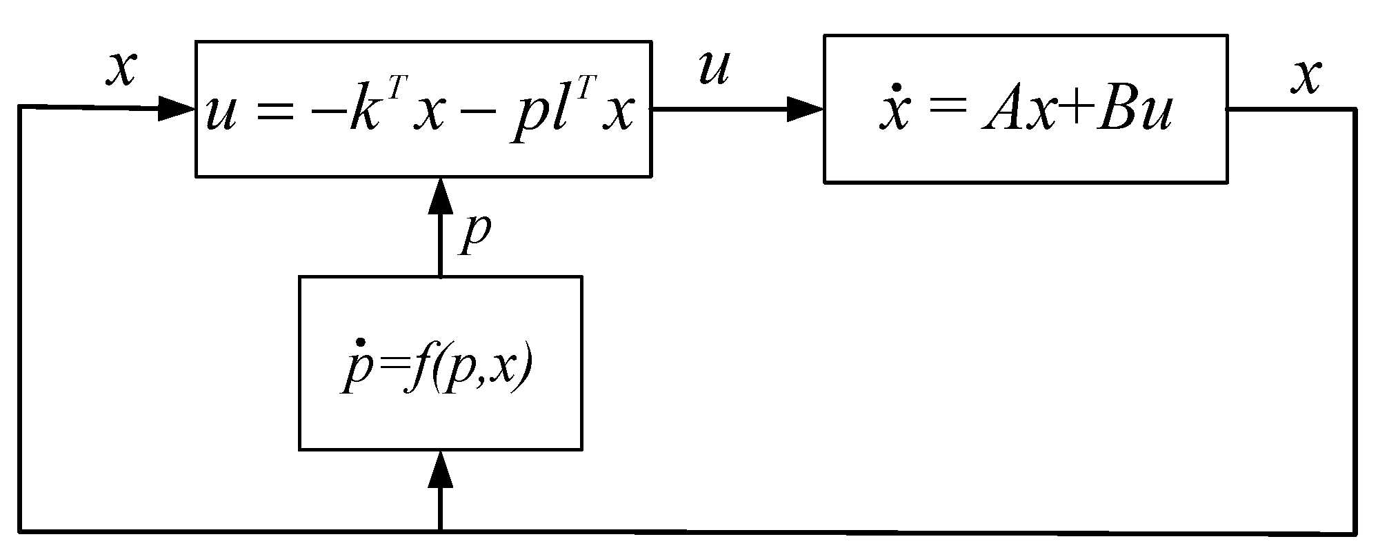
4. Design of the DSVSC

Dynamic soft variable structure control (DSVSC) is a control method based on soft variable structure control [23,24]. Compared with the SMC method, it uses differential equations as a dynamic selection strategy to avoid sliding modes. The way it changes controller parameters or structures is continuous, so the control signal of the DSVSC is smoother and more continuous, and the system can achieve or approach the performance of time-optimal control. The stability of the system was ensured through the Lyapunov direct method.

4.1. Overall Design of the DSVSC

Linear systems with N-dimensional discontinuous variable structure control or switching control are considered as follows:

$$\dot{x}=Ax+Bu$$

(24)

Existence: The constraint control |u| ≤ u₀ and controller u = F(x, p) are calculated according to the selection parameter p and the system state vector x. The p is defined by function S and calculated by selecting a strategy, as shown in Equation (25):

$$\dot{p}=f(p,x)$$

(25)

By determining the selection parameter p based on the continuous function S, the shortcomings of discontinuous variable structure control can be avoided.

According to the boundary of the initial value x₀, the DSVSC is:

$$u=-{\left(k+p·l\right)}^{T}x$$

(26)

In the equation, both k and l are control vectors. By combining Equations (24) and (26), it can be obtained that:

$$\dot{x}=\left(A-B{k}^T-pB{l}^T\right)x=\left(A_0-pB{l}^T\right)x$$

(27)

The control vector k needs to be able to stabilize A₀ = A − Bk^T. The differential equation obtained by combining Equations (25) and (27) is as follows:

$$\left[\begin{array}{c}\dot{x}\\ \dot{p}\end{array}\right]=\left[\begin{array}{c}{(A}_0-pB{l}^T)x\\ f(p,x)\end{array}\right]$$

(28)

The structure of the control system is shown in Figure 4.

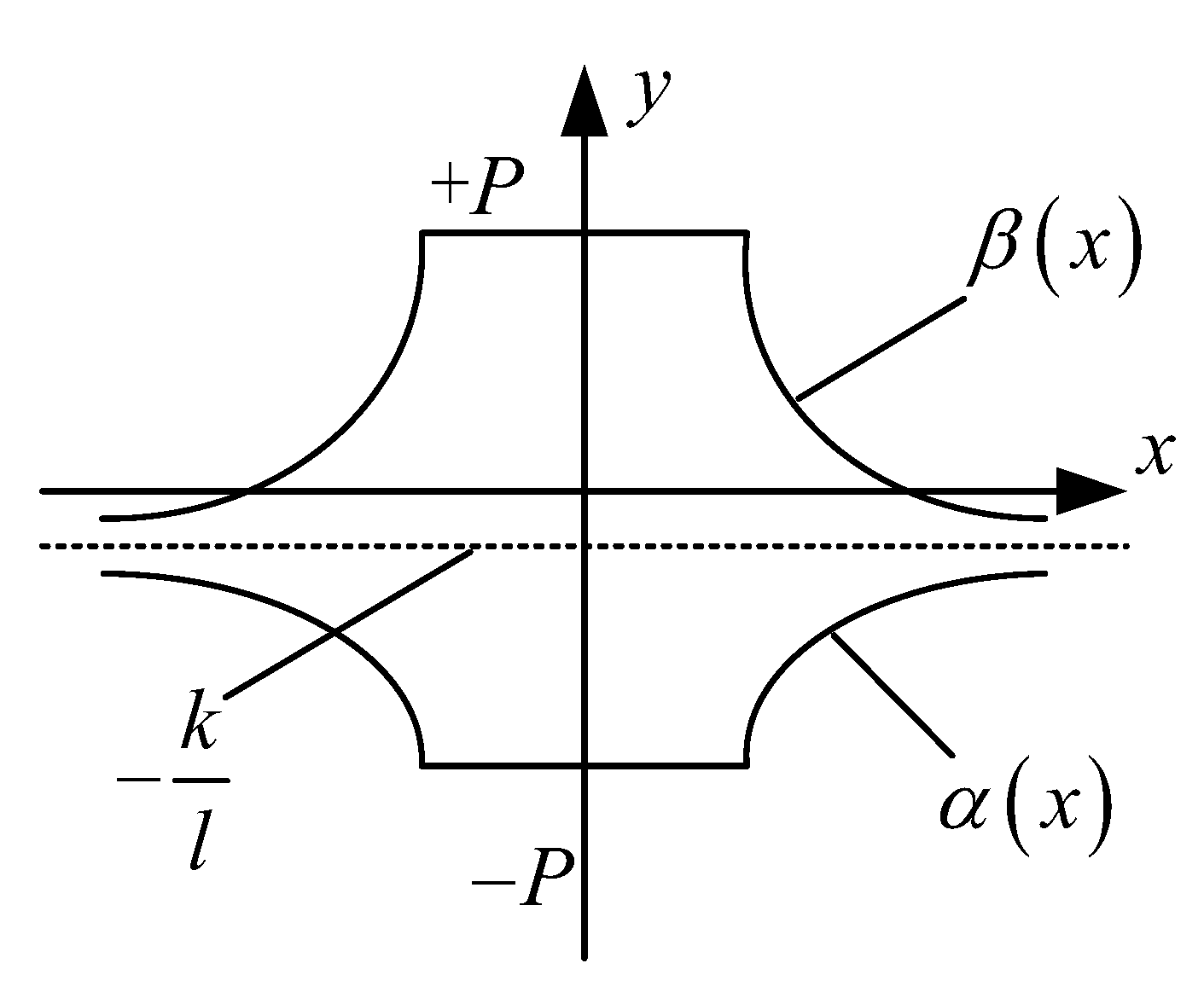
4.2. Design of the Selection Strategy for the DSVSC

The selection strategy is composed of function f, and its establishment process is as follows:

If Equation (28) has a single asymptotically stable equilibrium point:

$$\left[\begin{array}{c}x\\ p\end{array}\right]=\left[\begin{array}{c}0\\ 0\end{array}\right]$$

(29)

To meet this requirement, the Lyapunov function v(p, x) of the system is set as a positive, definite quadratic equation:

$$v\left(p,x\right)=x^{T}Rx+q{p}^2$$

(30)

According to Lyapunov’s asymptotic stability theorem, there is:

$$\dot{v}\left(p,x\right)={\dot{x}}^{T}Rx+x^{T}R\dot{x}+2qp\dot{p}<0$$

(31)

By introducing Equation (28) into Equation (31), it can be obtained that:

$$\dot{v}\left(p,x\right)=x^T\left(A_0^{T}R+R{A}_0\right)x-2p^{2}r\left(p,x\right)<0$$

(32)

In this inequality, the function r is:

$$-x^{T}RB{l}^{T}x+qf\left(p,x\right)=-p·r(p,x)$$

(33)

If $A_0^{T}R+R{A}_0=-Q$ is a negative definite matrix and $r\left(p,x\right)>0$, Equation (32) will be satisfied, and the control system Equation (28) will be stable.

For the first stability condition, since the eigenvalue of A₀ has a negative real part, there is a positive definite solution R for any positive definite matrix Q, which satisfies Equation (31).

For the second stability condition, the selection strategy can be obtained from Equation (33), as shown:

$$\dot{p}=f\left(p,x\right)=\frac{x^{T}RB{l}^{T}x-p·r\left(p,x\right)}{q}$$

(34)

In the equation, the control constraint |u| ≤ u₀ needs to be taken into account when selecting the function r. The inequality is obtained from (26):

$$\left\{\begin{array}{l}\frac{{-u_0-k}^{T}x}{l^{T}x}\le p\le \frac{{u_0-k}^{T}x}{l^{T}x}(l^{T}x>0)\\ \frac{{u_0-k}^{T}x}{l^{T}x}\le p\le \frac{{{-u}_0-k}^{T}x}{l^{T}x}(l^{T}x<0)\end{array}\right.$$

(35)

The constraint on the control signal u is replaced by the constraint on the selection variable p.

When x approaches the equilibrium point x = 0, the range defined by Equation (35) will expand extremely. The selection of variable p will obtain very large values, which will cause serious noise and disturbance. To avoid these effects, the system is required to impose constraints on the control variable p, as shown in Equation (36):

$$-P\le p\le P$$

(36)

where P is a larger positive number.

Combining inequalities (35) and (36), it can be obtained that:

$$\alpha \left(x\right)\le p\le \beta \left(x\right)$$

(37)

The state variable x is included in the following range:

$$\alpha \left(x\right)=\left\{\begin{array}{l}\frac{{u_0-k}^{T}x}{l^{T}x}\left(l^{T}x\le \frac{-{u_0+k}^{T}x}{P}\right)\\ -P\left(\frac{-{u_0+k}^{T}x}{P}<l^{T}x<\frac{{u_0+k}^{T}x}{P}\right)\\ \frac{-{u_0-k}^{T}x}{l^{T}x}\left(l^T\ge \frac{{u_0+k}^{T}x}{P}\right)\end{array}\right.$$

(38)

$$\beta \left(x\right)=\left\{\begin{array}{l}\frac{{{-u}_0-k}^{T}x}{l^{T}x}\left(l^{T}x\ge \frac{{u_0+k}^{T}x}{P}\right)\\ P\left(\frac{-{u_0-k}^{T}x}{P}<l^{T}x<\frac{{u_0-k}^{T}x}{P}\right)\\ \frac{{u_0-k}^{T}x}{l^{T}x}\left(l^T\ge \frac{{u_0-k}^{T}x}{P}\right)\end{array}\right.$$

(39)

Described in Equations (38) and (39), α(x) and β(x) functions are shown in Figure 5 below, both of which are functions of one variable corresponding to the x variable.

The range of p in the differential function f has been determined. The function r(p, x) > 0 is made, in which case both the inequality (37) and the constraint |u| ≤ u₀ are satisfied. The function r is as follows:

$$r\left(p,x\right)=\left\{\begin{array}{l}\mu \left(1-\frac{\alpha \left(x\right)}{p}\right)+{\mu }_0\frac{\alpha \left(x\right)}{p}\left(p\le \alpha \left(x\right)\right)\\ {\mu }_0 \left(\alpha \left(x\right)<p<\beta \left(x\right)\right)\\ \mu \left(1-\frac{\beta \left(x\right)}{p}\right)+{\mu }_0\frac{\beta \left(x\right)}{p}\left(p\ge \beta \left(x\right)\right)\end{array}\right.$$

(40)

Equation (34) is an anti-saturation system, as shown in Figure 6. The constant μ < 1 determines the range of the anti-saturation region. It can prevent the parameter value output by the integrator from falling below α(x) or exceeding β(x). The constant 0 < μ₀ < 1 limits the extent to which the anti-saturation system does not function so that the constraint inequality Equation (35) and (37), and stability condition inequality $r\left(p,x\right)>0$ are satisfied.

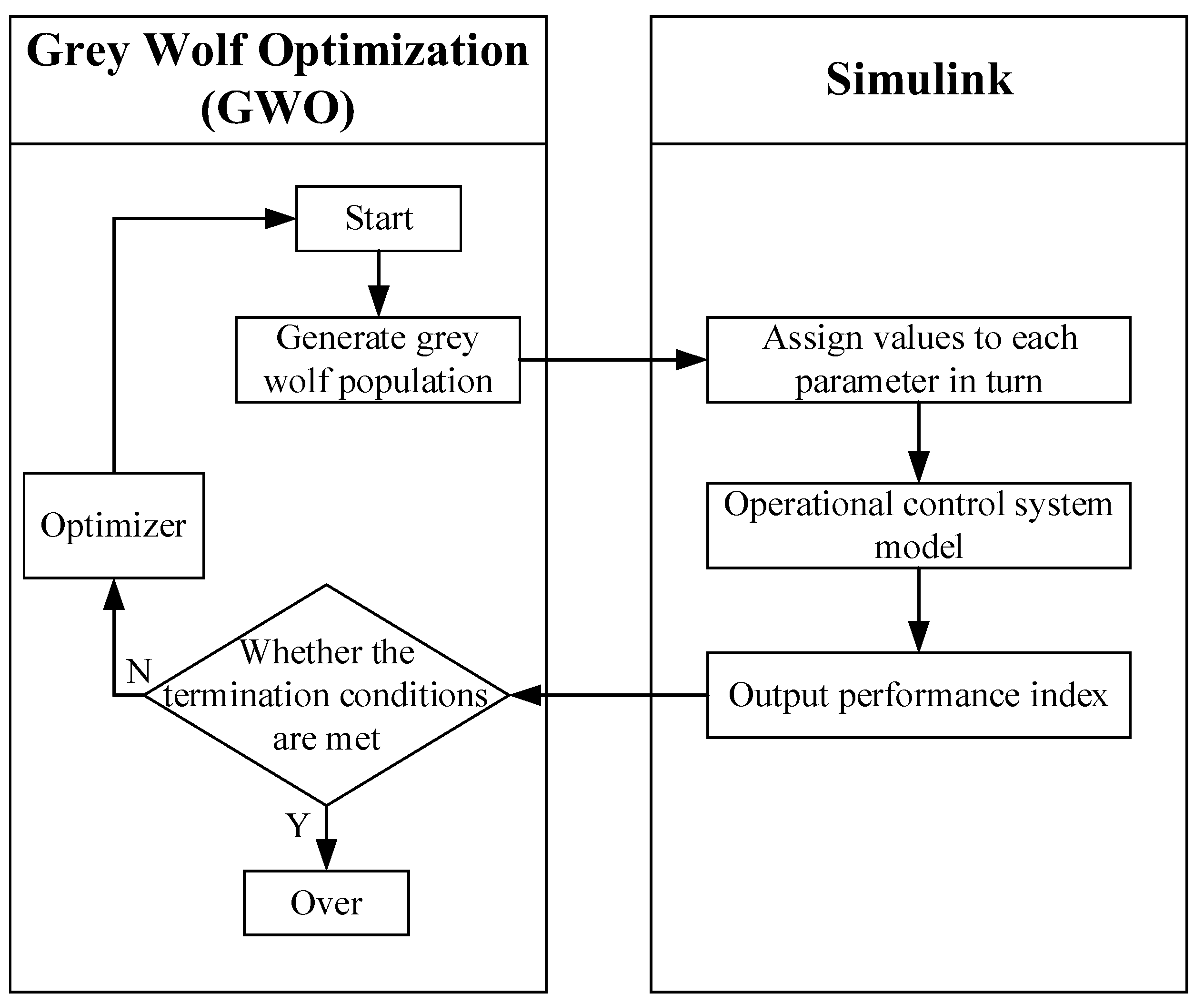
4.3. Setting of Control Parameters

When designing this controller, it was important to consider the linear control vectors k and l, the positive definite matrix R, the parameters q and p, and the parameters μ and μ₀ of the function r. In addition to the parameters obtained through calculation, some parameters needed to be designed, among which the control vectors k and l had a greater influence. The Grey Wolf optimization algorithm was used to assist with parameter setting, and the minimum tracking error was taken as the evaluation index to select each parameter. Finally, k = [−51: 1.38] and l = [18.7: −51.4] were selected, and their basic principle is shown in Figure 7.

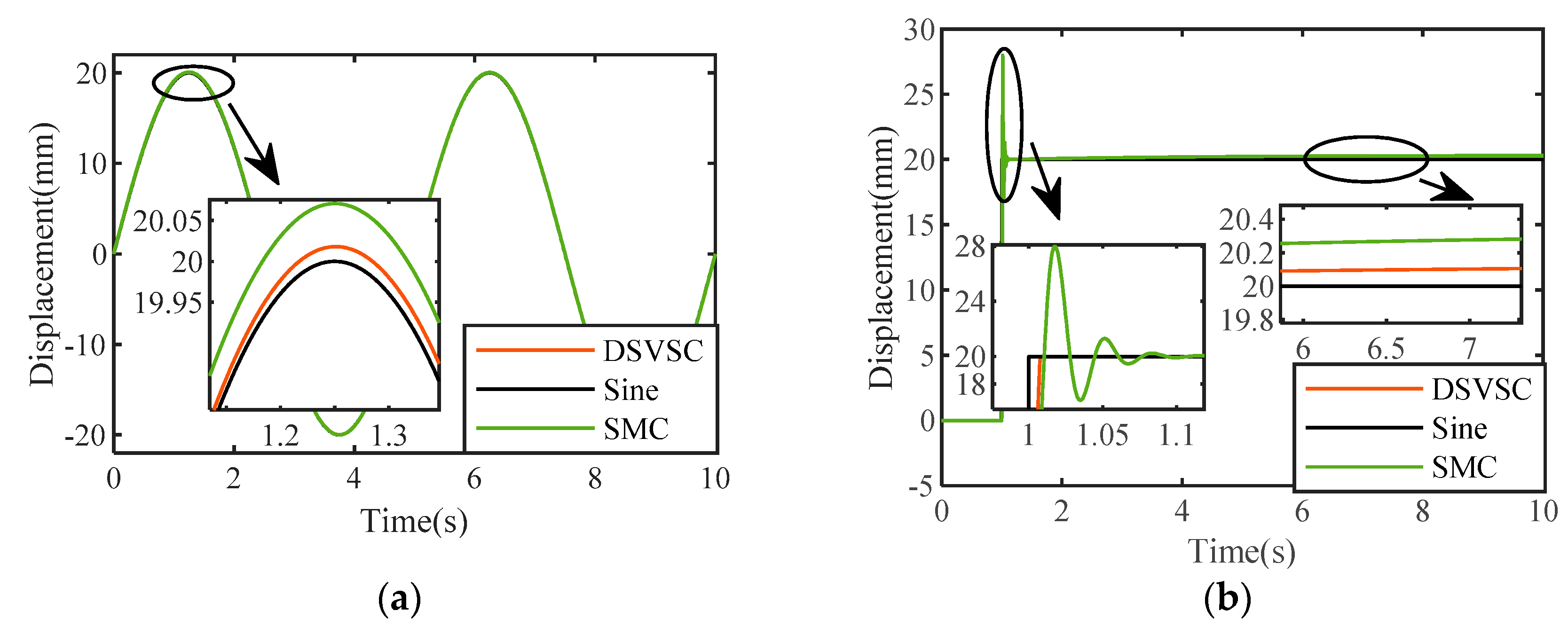
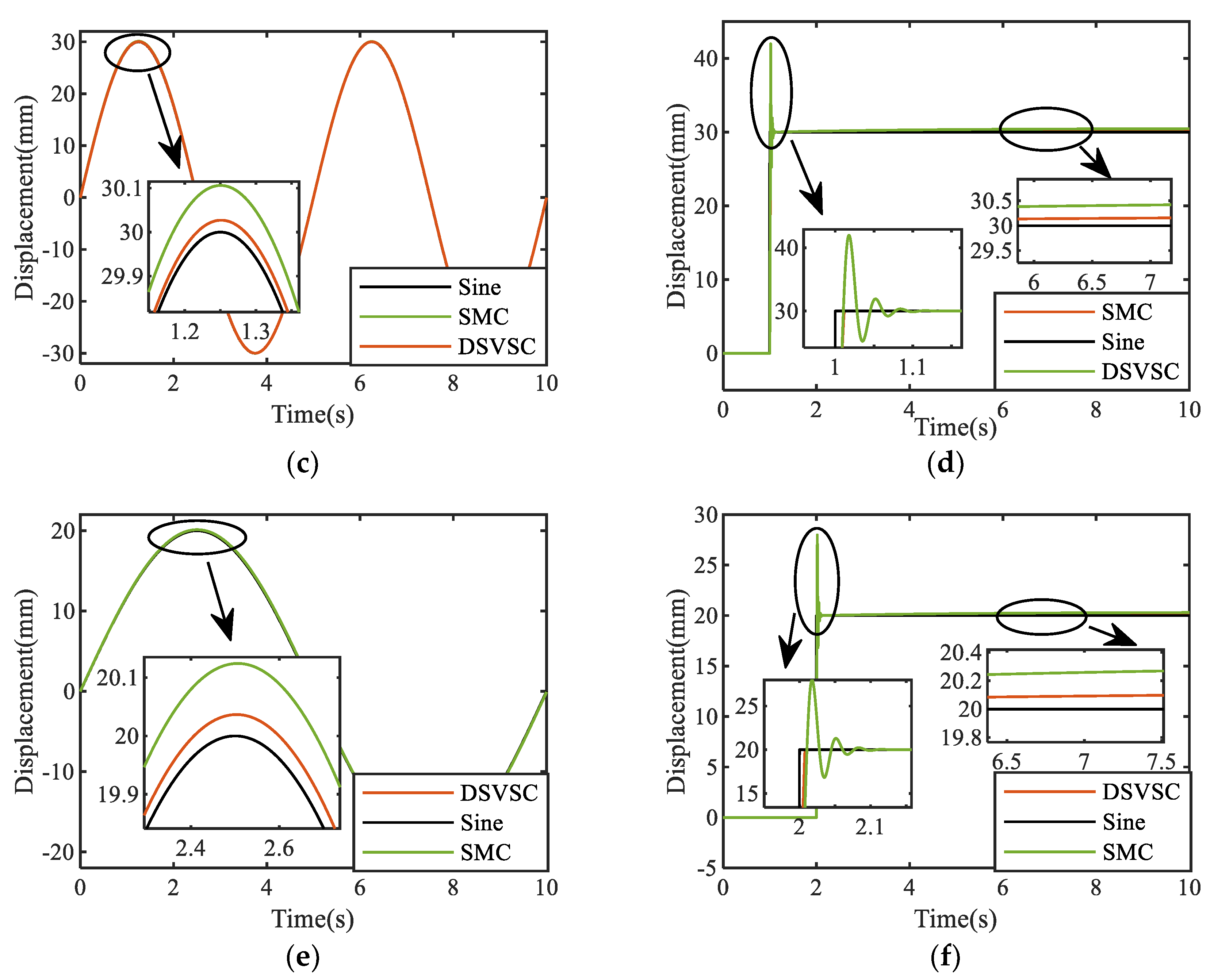
5. Simulation Analysis

In this section, a simulation model of the valve-controlled cylinder system and a controller simulation model were established using MATLAB/Simulink. By comparing the simulation results of the DSVSC and SMC, the effectiveness of the controller was verified.

The input source signals were step signal and sine signal, with a unified simulation time of 10 s and a sampling time of 0.001 s. The comparison of three sets of simulation response curves obtained by changing the step time and final value of the input step signal, as well as the amplitude and frequency of the input sine signal, are shown in Figure 8.

From Figure 8a, it can be seen that the sinusoidal response phase lag of the valve-controlled cylinder system based on the DSVSC is approximately 0.005°, and the amplitude error is approximately 0.1%. The phase lag of the sinusoidal response based on SMC is approximately 0.006°, and the amplitude error is approximately 0.43%.

It can be seen from Figure 8b that the steady-state value of the step response of the valve-controlled cylinder system based on the DSVSC is 20.1 mm, the rise time is approximately 1.01 s, the maximum overshoot is 0.5%, and the adjustment time is approximately 1.02 s. The steady-state value of the step response based on SMC is 20.25, the rise time is approximately 1.015 s, the maximum overshoot is 40%, and the adjustment time is approximately 1.1 s.

From the other two sets of figures, it can be seen that when a sine signal was input, the amplitude error of the output signal increased when the amplitude of the sine signal increased or the frequency decreased, while the phase lag of the output curve remained basically unchanged. When inputting a step signal, as the final value of the step signal increased, the steady-state error and overshoot of the output curve increased. The starting step time of the step signal did not affect the evaluation index of the output curve, and the rise time and steady-state time of the output curve remained basically unchanged. From the simulation results, it can be seen that both the DSVSC and SMC had good response speeds, but the SMC had some shortcomings, such as excessive overshoot. The DSVSC had a smaller overshoot and better tracking effect in the valve-controlled cylinder system, and overall, its performance was superior to the SMC.

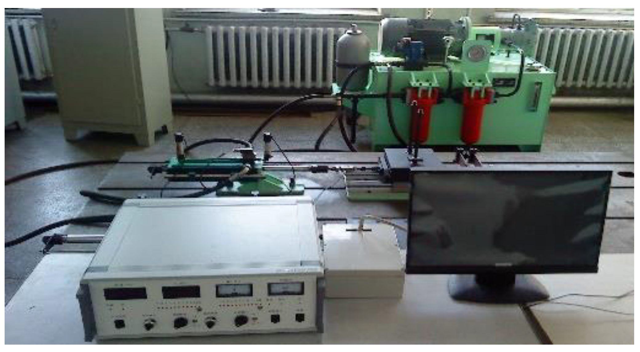
6. Experimental Verification

To verify the actual control effects of the two controllers designed, this section mainly conducted experimental verification of the signal tracking effects of the two controllers designed through the electro-hydraulic servo position control system experimental platform.

6.1. Composition of the Experimental Platform

Figure 9 shows a physical image of the experimental platform. The experimental platform mainly consists of a hydraulic pump station, a valve-controlled cylinder section, and a control section. The system collects signals from sensors through the RTW real-time window in MATLAB and sends out signals to control the electro-hydraulic servo valve to achieve movement of the valve-controlled cylinder.

This experimental platform was conducted in an XPC semi-physical simulation environment. By combining the RTW real-time window in MATLAB with Simulink, the system software and hardware were coordinated to achieve real-time control. The component models of the experimental platform are shown in

Table 2. The component type of the electro-hydraulic servo test bench.

Part	Name	Model
Hydraulic pump station	Motor	Y2-160L-4
	Hydraulic pump	PCY14-1B
	Relief valve	DBD-type direct acting relief valve
Valve-controlled cylinder section	Electro-hydraulic servo valve	FF102-30-type double nozzle baffle servo valve
	Displacement sensor	FXB-V71/100
Control section	Data acquisition card	PCL-1710HG
	IPC	IPC-610H
	Industrial motherboards	PCA-6114P4-B

.

6.2. Experimental Verification of Controllers for the Valve-Controlled Cylinder Position System

Sinusoidal and step signals with different parameters were input to observe the change in the response curve, and the experimental time was uniformly set to 10 s. A comparison of the response curves of the DSVSC and SMC is shown in Figure 10.

Set Figure 10a,b as Group 1 of experiments, Figure 10c,d as Group 2 of experiments, and Figure 10e,f as Group 3 of experiments. The data results are shown in

Table 3. Experimental response results when the sinusoidal signal was input.

Input Signal	Evaluating Indicator	Group Number	DSVSC	SMC
Sine	Amplitude attenuation (%)	Group. 1	−1.5	−3.0
		Group 2	−2.5	−3.0
		Group 3	−1.9	−2.9
	Phase lag (°)	Group 1	0.03	−0.04
		Group 2	0.02	−0.02
		Group 3	0.07	−0.02

and

Table 4. Experimental response results when the step signal was input.

Input Signal	Evaluating Indicator	Group Number	DSVSC	SMC
Step	Amplitude attenuation (%)	Group 1	20	19.86
		Group 2	20	19.86
		Group 3	30	29.86
	Phase lag (°)	Group 1	2.064	2.051
		Group 2	3.564	3.554
		Group 3	2.072	2.0625
	Peak time (s)	Group 1	2.096	2.088
		Group 2	3.598	3.588
		Group 3	2.1035	2.091
	Overshoot (%)	Group 1	0.179	2.2
		Group 2	0.118	1.5
		Group 3	2.85	2.91
	Adjust time (s) (Δ = 0.05)	Group 1	2.07	2.056
		Group 2	3.571	3.561
		Group 3	2.08	2.0691

.

From Figure 8 and Figure 10 and Table 3 and Table 4, it can be seen that the experimental results meet the expectations of the simulation. When a sine signal was input, the amplitude error of the output curve increased when the amplitude of the sine signal increased or the frequency decreased, and the phase lag of the output curve increased when the amplitude or frequency of the sine signal increased. When inputting a step signal, as the amplitude of the step signal increased, the amplitude attenuation and overshoot of the output curve increased, and the rise time and steady-state time of the output curve remained basically unchanged. In addition, compared to the simulation results, it can be found that the control error of the experimental results was greater than that of the simulation, and the SMC always had an obvious chattering phenomenon in the curve. It can be concluded that the factors ignored during the simulation had an impact on the actual control effect of the controller. The DSVSC in the valve-controlled cylinder position servo system had a smaller overshoot, a better tracking effect, and a smoother response curve after reaching a steady state.

7. Conclusions

In this paper, the DSVSC and SMC, based on variable structure control principles, were designed for high-precision control of valve-controlled cylinders. First, the mathematical model of the electro-hydraulic servo control system was established based on its operating mechanism, and the design of the sliding mode surface and reaching law in SMC was completed based on the system’s mathematical model. In the design of DSVSCs, continuous differential equations were used as the selection strategy to avoid the occurrence of sliding mode dynamics. The stability of the system was ensured through the Lyapunov method, and the parameters in the DSVSC were tuned using the GWO algorithm. The simulation analysis was conducted in MATLAB, and experimental verification was conducted on the experimental platform. The simulation analysis and experimental verification results showed that the DSVSC had a smaller overshoot and better tracking effect in the control system, and the response curve after reaching a steady state was smoother. The DSVSC was a good control method that can ensure the position control effect of the system and eliminate the chattering phenomenon in SMC.

Finally, through the analysis of the controller designed in this study, it was found that there was chattering phenomenon in the designed SMC, especially when inputting step signals. Improvements need to be made to the design of sliding mode surfaces and reaching laws in SMC, such as adaptive adjustment algorithms for reaching the coefficient, quadratic sliding film form, terminal sliding film form, and integral sliding film form. In the DSVSC, the selection strategy is complex, there are many parameters that need to be adjusted, and it has a significant impact on the system control effect. Therefore, parameter tuning can be improved.

References

1. Karpenko, M.; Stosiak, M.; Šukevičius, Š.; Skačkauskas, P.; Urbanowicz, K.; Deptuła, A. Hydrodynamic Processes in Angular Fitting Connections of a Transport Machine’s Hydraulic Drive. Machines 2023, 11, 355. [Google Scholar] [CrossRef]
2. Bury, P.; Stosiak, M.; Urbanowicz, K.; Kodura, A.; Kubrak, M.; Malesińska, A. A Case Study of Open-and Closed-Loop Control of Hydrostatic Transmission with Proportional Valve Start-Up Process. Energies 2022, 15, 1860. [Google Scholar] [CrossRef]
3. Hou, S.; Chen, C.; Chu, Y.; Fei, J. Experimental validation of modified adaptive fuzzy control for power quality improvement. IEEE Access 2020, 8, 92162–92171. [Google Scholar] [CrossRef]
4. Pal, A.K.; Naskar, I.; Paul, S. A Fuzzy-Based Modified Gain Adaptive Scheme for Model Reference Adaptive Control. In Information and Decision Sciences: Proceedings of the 6th International Conference on FICTA; Springer: Singapore, 2018; pp. 315–324. [Google Scholar]
5. Bai, S.; Ben-Tzvi, P.; Zhou, Q.; Huang, X. Variable structure controller design for linear systems with bounded inputs. Int. J. Control. Autom. Syst. 2011, 9, 228–236. [Google Scholar] [CrossRef]
6. Adamy, J.; Flemming, A. Soft variable-structure controls: A survey. Automatica 2004, 40, 1821–1844. [Google Scholar] [CrossRef] [Green Version]
7. Fan, Y.; Shao, J.; Sun, G. Optimized PID controller based on beetle antennae search algorithm for electro-hydraulic position servo control system. Sensors 2019, 19, 2727. [Google Scholar] [CrossRef] [PubMed] [Green Version]
8. Yao, B.; Bu, F.; Chiu, G.T. Non-linear adaptive robust control of electro-hydraulic systems driven by double-rod actuators. Int. J. Control 2001, 74, 761–775. [Google Scholar] [CrossRef]
9. Gao, B.; Shao, J.; Yang, X. A compound control strategy combining velocity compensation with ADRC of electro-hydraulic position servo control system. ISA Trans. 2014, 53, 1910–1918. [Google Scholar] [CrossRef] [PubMed]
10. Peng, X.B.; Gong, G.F.; Yang, H.Y.; Lou, H.Y.; Wu, W.Q.; Liu, T. Quantitative feedback controller design and test for an electro-hydraulic position control system in a large-scale reflecting telescope. Front. Inf. Technol. Electron. Eng. 2017, 18, 1624–1634. [Google Scholar] [CrossRef]
11. Tri, N.M.; Nam, D.N.C.; Park, H.G.; Ahn, K.K. Trajectory control of an electro hydraulic actuator using an iterative backstepping control scheme. Mechatronics 2015, 29, 96–102. [Google Scholar] [CrossRef]
12. Utkin, V. Variable structure systems with sliding modes. IEEE Trans. Autom. Control 1977, 22, 212–222. [Google Scholar] [CrossRef]
13. Utkin, V. Discussion aspects of high-order sliding mode control. IEEE Trans. Autom. Control 2015, 61, 829–833. [Google Scholar] [CrossRef]
14. AQiu, H.D.; Zhang, X.G.; Fan, Y.X. Research on Electro-hydraulic Position Synchronous Servo System Based on Feedback Linearization Sliding Mode Control. Mach. Build. Autom. 2022, 51. [Google Scholar]
15. Xiong, J.J.; Zhang, G.B. Global fast dynamic terminal sliding mode control for a quadrotor UAV. ISA Trans.-Actions 2017, 66, 233–240. [Google Scholar] [CrossRef] [PubMed]
16. Yi, G.A.N.; Yang, C.H.E.N.; Fujia, S.U.N. Research of interference torque on car camera stabilized platform based on variable structure control. Mach. Des. Manuf. 2019, 1, 111–114. [Google Scholar]
17. Gao, B.; Guan, H.; Tang, W.; Han, W.; Xue, S. Research on Position Recognition and Control Method of Single-leg Joint of Hydraulic Quadruped Robot. Recent Adv. Electr. Electron. Eng. Former. Recent Pat. Electr. Electron. Eng. 2021, 14, 802–811. [Google Scholar] [CrossRef]
18. Milecki, A.; Ortmann, J. Electrohydraulic linear actuator with two stepping motors controlled by overshoot-free algorithm. Mech. Syst. Signal Process. 2017, 96, 45–57. [Google Scholar] [CrossRef]
19. Hongcheng, Y.; Xiaoxian, Y. Modeling and Simulation of Double Nozzle Flapper Gas Servo Valve. In Proceedings of the 2017 International Conference on Computer Systems, Electronics and Control (ICCSEC), Dalian, China, 25–27 December 2017; IEEE: Piscataway, NJ, USA, 2017; pp. 210–215. [Google Scholar]
20. Jelali, M.; Kroll, A. Hydraulic Servo-Systems: Modelling, Identification and Control; Springer Science & Business Media: Berlin/Heidelberg, Germany, 2002; pp. 69–72. [Google Scholar]
21. El Makrini, I.; Rodriguez-Guerrero, C.; Lefeber, D.; Vanderborght, B. The variable boundary layer sliding mode control: A safe and performant control for compliant joint manipulators. IEEE Robot. Autom. Lett. 2016, 2, 187–192. [Google Scholar] [CrossRef]
22. Kali, Y.; Rodas, J.; Gregor, R.; Saad, M.; Benjelloun, K. Attitude tracking of a tri-rotor UAV based on robust sliding mode with time delay estimation. In Proceedings of the 2018 International Conference on Unmanned Aircraft Systems (ICUAS), Dallas, TX, USA, 12–15 June 2018; pp. 346–351. [Google Scholar]
23. Liu, Y.L.; Gao, C.C.; Meng, B.; Cong, X.W. Dynamic soft variable structure control for singular systems. In Proceedings of the 30th Chinese Control Conference, Shenyang, China, 9–11 June 2018; pp. 2572–2577. [Google Scholar]
24. Lee, H.; Utkin, V.I. Chattering suppression methods in sliding mode control systems. Annu. Rev. Control 2007, 31, 179–188. [Google Scholar] [CrossRef]
Figure 1. Schematic diagram of the electro-hydraulic servo position system.
Machines 11 00623 g001
Figure 2. Structure diagram of the electro-hydraulic position servo system.
Machines 11 00623 g002
Figure 3. Block diagram of the transfer function for the electro-hydraulic servo system.
Machines 11 00623 g003
Figure 4. Structure diagram of the dynamic soft variable structure control system.
Machines 11 00623 g004
Figure 5. Diagram of function α(x) and function β(x).
Machines 11 00623 g005
Figure 6. Structure of the differential equation p ˙ = f ( p , x ) .
Machines 11 00623 g006
Figure 7. Block diagram of adjusting the DSVSC parameters using the grey wolf algorithm.
Machines 11 00623 g007
Figure 8. Response curves of the simulation results for the two controllers: (a) Sinusoidal signal response curve (amplitude 20 mm, frequency 0.4 pi rad/sec); (b) Step signal response curve (step time 1 s, final value 20 mm); (c) Sinusoidal signal response curve (amplitude 30 mm, frequency 0.4 pi rad/sec); (d) Step signal response curve (step time 1 s, final value 30 mm); (e) Sinusoidal signal response curve (amplitude 20 mm, frequency 0.2 pi rad/sec); (f) Step signal response curve (step time 2 s, final value 20 mm).
Machines 11 00623 g008aMachines 11 00623 g008b
Figure 9. Physical diagram of the electro-hydraulic position servo system experimental bench.
Machines 11 00623 g009
Figure 10. Response curves of the experimental results for the two controllers: (a) Sinusoidal response curve (amplitude 20 mm, frequency 0.4 pi rad/sec); (b) Step signal response curve (step time 2 s, final value 20 mm); (c) Sinusoidal response curve (amplitude 20 mm, frequency 0.2 pi rad/sec); (d) Step signal response curve (step time 3.5 s, final value 20 mm); (e) Sinusoidal response curve (amplitude 30 mm, frequency 0.4 pi rad/sec); (f) Step signal response curve (step time 2 s, final value 30 mm).
Machines 11 00623 g010