Article

A Study of Knee Exoskeleton Configuration Based on Lower Limb Motion Characteristics Analysis

1
School of Mechanical and Precision Instrument Engineering, Xi’an University of Technology, Xi’an 710048, China
2
Department of Industrial Design, Xi’an University of Technology, Xi’an 710054, China
*
Author to whom correspondence should be addressed.
Machines 2023, 11(7), 709; https://doi.org/10.3390/machines11070709
Submission received: 27 May 2023 / Revised: 27 June 2023 / Accepted: 1 July 2023 / Published: 4 July 2023
(This article belongs to the Section Machine Design and Theory)

Abstract

:
In order to solve poor coordination between the exoskeleton and the human leg, this article analyzed the spatiotemporal characteristics of lower limb motion using data collection from human walking gait experiments. According to the macro- and micro-motion mechanisms of the knee joint, six knee exoskeleton configurations were proposed. Combined with the analysis of gait characteristics, mathematical models for lower limb kinematics and dynamics were established and verified with numerical simulation. Using human–machine coupling simulation experiments, different knee exoskeleton devices were simulated for wear, and a configuration of the exoskeleton mechanism compatible with human knee motion was selected, which improved human–machine adaptability and coordination. This study provides a new method for studying adaptive knee exoskeletons.

1. Background

The research on human musculoskeletal systems has gone through the stages of rigid body kinematics, rigid body dynamics, and skeletal muscle kinematics and dynamics. A lower limb exoskeleton robot can help patients with lower limb motor dysfunction, which can provide assisted forces during movement. During the design and development of exoskeletons, the primary considerations are to reduce the generation of harmful forces from the perspective of institutional motion, suppress contact collision forces at the joints, and improve wear comfort and product performance. Secondly, when wearing an exoskeleton, the exoskeleton needs to follow the lower limbs to complete a walking movement, so it needs to be able to meet the requirements for freedom of movement with the wearer. Due to the important role of the knee joint in lower limb movement, modeling and assisting knee joint components has become one of the most important components in exoskeleton mechanisms, and the related research is relatively extensive. In 1836, the Weber brothers first discovered that the motion of the knee joint is not simply a rotation but a combination of rolling and sliding motion forms [1]. Since then, many scholars have studied and explored the complex forms of motion of the knee joint. Early research on human knee joint models can be traced back to 1950, when Bresler et al. [2] established a simple biomechanical model of the human knee joint. After that, many scholars also conducted research on knee joint models and proposed various knee joint models. Typical models include hinge joints, translation joints, spherical joints, and viscoelastic joints. Because the hinge model does not consider the geometric shape of the knee joint or the ligament function of the knee joint engagement, it can only be used to predict the force exerted on the knee joint during human walking [3].
Currently, in the design of existing exoskeleton mechanisms, the knee joint motion model is simplified to a rotating pair with an axis perpendicular to the sagittal plane and a fixed axis position [4,5]. For example, the rehabilitation exoskeleton developed by James et al. [6] is called the Series Elastic Remote Knee Actuator (SERKA). Considering the kinematic characteristics of the knee joint, the knee joint kinematics model can be viewed as a variable axis rotation pair with instantaneous centers continuously changing in the sagittal plane. For example, Chaichaowarat et al. [7] developed an exoskeleton prototype using a cross-four-bar mechanism, Wang et al. [8] proposed an adaptive mechanism with a slider/cam, and Yu et al. [9] proposed a noncircular gear-five-bar mechanism. To approach the microscopic motion mechanism of the knee joint more closely, the knee kinematics model is used, which is a rotating joint whose axis position and posture change instantaneously in space with the joint rotation angle [10,11,12]. Shafiei et al. [13] found that adding backlash to the connecting elements of a lower limb robot exoskeleton can significantly improve the performance indicators of the robot exoskeleton. To improve alignment on all three planes, a design with six degrees of freedom is always used.
Most mechanisms only ensure that the axis of the exoskeleton joint is aligned with the axis of the knee joint in the sagittal plane without considering the positional changes in the knee joint axis in other planes. During the wearing movement process, due to the inability to align the joint axes in real-time, man–machine coordination is poor, thus affecting the wearing comfort and causing secondary harm to the human body. Zhang et al. [14] concluded that more than 77% of the devices did not consider alignment in the DOF design of knee-assisted devices, about 11% and 4% used single DOF mechanisms and under-actuation mechanisms, respectively, and only 8% used other methods to achieve knee alignment. Existing mechanisms draw on the kinematic structural characteristics of the human knee exoskeleton to obtain a simplified mechanism model.
On the basis of traditional cross-four-link linkage, many scholars have conducted further in-depth research. For example, Jiang et al. [15] proposed an improved five-bar model that can effectively simulate a biological knee joint. Shin et al. [16] proposed an optimization design method for multi-link knee joints. Similarly, many scholars are now looking for configuration solutions that are closer to biological knee joint activity from different perspectives. However, from the mechanism configuration design perspective, the existing research has rarely explored the methods and approaches for aligning external skeletal joints with human joints during movement. There is a lack of comparative analysis methods for the impact of force magnitude on the human interface junction.
This study aims to analyze joint motion characteristics and time-varying characteristics during lower limb walking. First, the kinematic and dynamic models of the lower limb were established, and the reliability of the models was verified with simulation. Secondly, the exoskeleton mechanism configuration schemes based on the macroscopic and microscopic motion mechanisms of the knee joint were proposed, and the human–machine motion adaptability of each scheme was evaluated with simulation. The second part of this article analyzes the lower limb motion characteristics. The third part introduces the establishment of mathematical models for lower limb kinematics and dynamics. The fourth part introduces and discusses the design, data processing, and results of the human–machine coupling simulation experiments. In the fifth part, the conclusion of this article is drawn.

2. Analysis of the Biomechanical Characteristics of Lower Limb Movement

2.1. Physiological Characteristics of Knee Joint Movement

The human knee joint is composed of the lower end of the femur, the upper end of the tibia, and the patella. The main internal structure of the knee is the meniscus and four ligaments. The meniscus, including the medial meniscus (MM) and lateral meniscus (LM), is the fibrocartilage tissue cushioned between the lower end of the femur and the upper end of the tibia inside the knee, which is used to cushion the vibration of the knee joint and avoid direct friction between the two bones. It is supported by four main ligaments. There are two ligaments on both sides of the knee, called the medial collateral ligament (MCL) and the lateral collateral ligament (LCL), whose main function is to prevent the knee axis from dislocating. The other two ligaments are distributed in the front and rear of the knee, called the anterior cruciate ligament (ACL) and posterior cruciate ligament (PCL), which prevent the knee from moving forward and backward. The specific structure is shown in Figure 1a. Chen et al. [17] pointed out that the motion forms of the knee joint include both rolling and sliding, and the main flexion and extension movement is in the sagittal plane. According to this feature, the research on the knee joint is mainly based on movement in the sagittal plane. During motion in the sagittal plane of the knee joint, the instantaneous rotation center of the leg relative to the thigh motion is not a constant point, and the instantaneous center trajectory curve is a “J” curve [18], as shown in Figure 1b.
Table 1 lists the ideal instantaneous center coordinate of the human knee joint [19], and the position in the sagittal plane is represented by ( x p , y p ). Since the reference coordinate system for the theoretical coordinate is located at the position of the lower leg of the human body, it is different from the absolute coordinate system O-xy in the exoskeleton kinematics model established above. Therefore, it is necessary to establish a local coordinate system for the knee joint with a variable axis and transform the coordinates of the instantaneous center point p in the absolute coordinate system O-xy, in order to optimize the calculation of rod length in the future.

2.2. Motion Space–Time Data Acquisition

The participant in this experiment is a male, aged 25 years, with a height of 180 cm and a weight of 75 kg, who is healthy and free from any other diseases. Before the experiment began, we provided the participant with a detailed introduction to the experimental methods and processes and then started the experiment process after ensuring familiarity with the experimental methods and processes. All methods were approved by Institutional Review Board (IRB), and the subject filled out an informed consent form.
A three-dimensional (3D) motion acquisition and analysis system (VICON T40S, VICON, UK) was used for gait data acquisition. The system consists of ten Vicon MX high-speed motion capture cameras, three AMTI plantar force measuring plates, optical trackers, computers, marking points, correction frames, and other auxiliary equipment, as shown in Figure 2a. The shooting frequency of the motion capture camera is 100 Hz, and the data collection frequency of the force measuring plate is 1500 Hz. The participant carried reflective marker balls, which were used to capture and record each marker point on the human body by reflecting light with the same wavelength onto the camera, as shown in Figure 2b. The data were processed into .C3D format files using point filling, correction, etc., in Vicon Nexus, and then the required motion data were obtained using motion analysis software. Each walking task consisted of 50 walking cycles, with a rest interval of about 2 min between each walking cycle. To avoid large fluctuations in the collected kinematics and dynamics data due to experimental fatigue, we attempted to ensure the subject’s natural gait during the experiment.
During the experiment, on the basis of using the VICON standard protocol, the subject’s lower limbs were equipped with the modified Cleveland Clinic pelvis and leg marking set (left and right ASIS, left and right greater trochanter, left and right PSI, pubic marker points, thigh marker points, medial and lateral epicondyle, lower leg marker points, medial and lateral malleolus, calcaneus, foot, fifth metatarsal) (Figure 2b). After the static standing test was calibrated, Visual 3D (C-Motion Inc., Germantown, MD, USA) modeling software was used to reconstruct the joint kinematics, dynamics, and centroid trajectory, assuming that the left and right legs were symmetrical.
Slight movements in the participant’s shoes and pants relative to their body are unavoidable. Therefore, during the motion capture experiment, the participant wore tight shorts and shoes that were highly matched with their body, so as to maximize movement consistent with the human body. Figure 2b shows the spatial trajectories of the marker points (marked in blue) that are the experimental data mainly used in this article. These marker positions were placed on the surface of the skin to minimize the artifacts of soft tissue movement from the bones. The marker points placed on the shoes and trousers were matched with the marker points in the biomechanical simulation software. Then, the biomechanical analysis software carried out the kinematics and dynamics analyses. This method for obtaining kinematics and dynamics data is widely accepted.

2.3. Movement Gait Characteristics Analysis

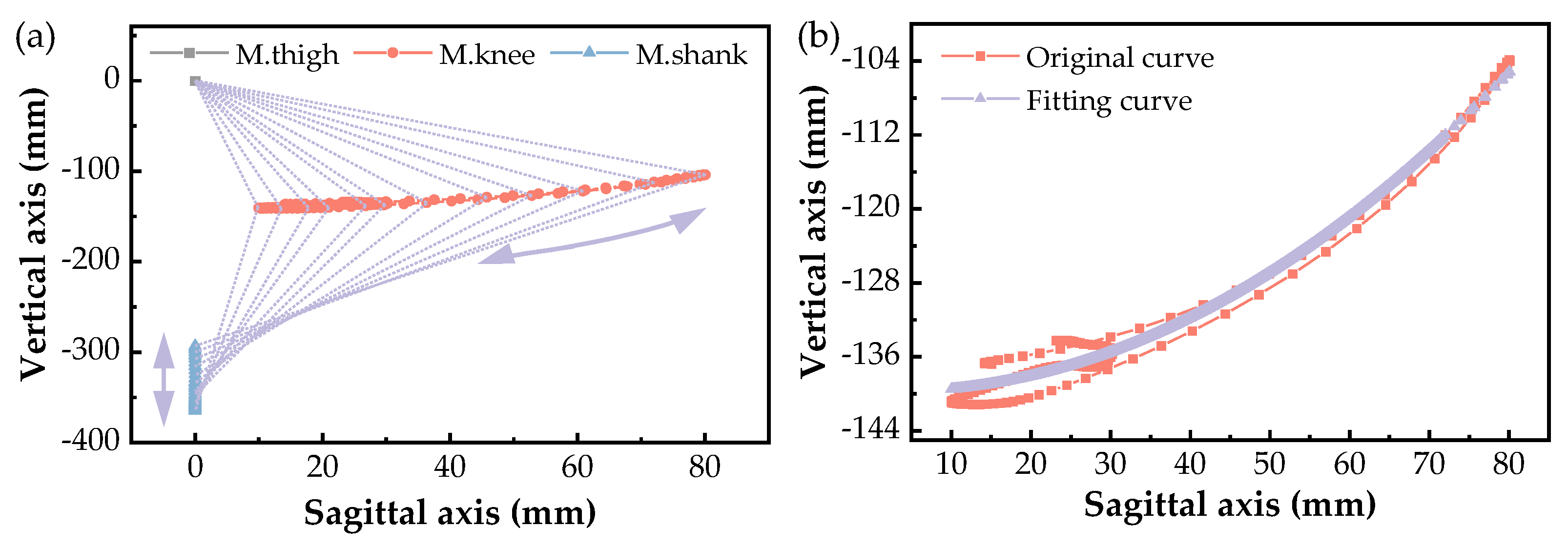
VICON motion capture equipment was used to obtain spatiotemporal data for each marker point, and the spatial data points for the thigh, knee joint, and shank marker points in a single gait cycle were selected as the research objects. According to the theory of human anatomy, human movement involves three basic planes and three basic axes [20].
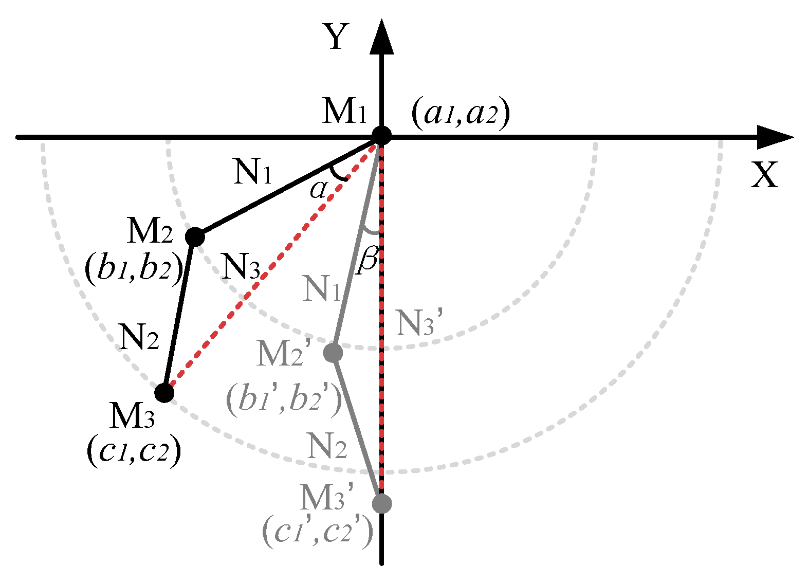
Figure 3 shows the spatiotemporal data for each marker point in the sagittal plane. The marker points at the thigh, knee joint, and shank are named M. thick, M. knee and M. shank, respectively, which define the thigh (M. thick), knee (M. knee), and shank (M. shank) marker points at any position as points M 1 ( a 1 , a 2 ) , M 2 ( b 1 , b 2 ) , and M 3 ( c 1 , c 2 ) , respectively. To solve the relative motion of the knee and shank when obtaining the fixed thigh marker point motion, we fixed the thigh marker point and ensured that the shank marker point fell on the y-axis, as shown in Figure 4.
Based on the geometric motion relationship in Figure 4, combined with the known spatial coordinates of M 1 , M 2 , and M 3 , the lengths N 1 , N 2 , and N 3 of the three connecting rods can be obtained using Equations (1)–(3).
N 1 = ( b 2 a 2 ) 2 + ( b 1 a 1 ) 2
N 2 = ( c 2 b 2 ) 2 + ( c 1 b 1 ) 2
N 3 = ( a 2 c 2 ) 2 + ( a 1 c 1 ) 2
The triangle formed with the marked points on the thigh, shank, and knee joints, combined with Equation (4), can be used to calculate the angle α between connecting rods N 1 and N 3 as follows:
α = arccos ( N 1 2 + N 3 2 N 2 2 2 N 1 N 3 ) α m i n
When a person stands on one foot while walking, the angle of the knee joint is defined as 0°. Therefore, assuming that the angle α remains unchanged after coordinate transformation, there will be a minimum value α m i n for angle α
.
β = α α m i n
N 3 = N 1 cos β + N 2 2 N 1 2 sin β 2 )
b 1 = N 1 sin α
b 2 = N 1 cos α
Therefore, the motion trajectory of the marked point at the end of the shank is M 3 ( 0 , N 3 ) , which is shown in Figure 5a as a reciprocating motion. Using Equations (7) and (8), the motion trajectory M 2 ( b 1 , b 2 ) of the knee joint is obtained, as shown in Figure 5b for nonlinear motion. When wearing a single degree of freedom knee exoskeleton, it is necessary to consider the joint matching error between the exoskeleton and the knee joint, as well as the sliding displacement at the lower leg.

2.4. Four-Link Mechanism Simulating the Knee Joint

By selecting a cross-four-bar linkage structure [21], the wearable knee exoskeleton can adopt a multi-center knee joint CoR to provide kinematics compatibility with the anatomical knee joint, so as to achieve ultimate knee flexion. A simulation of the CoR trajectory after moving the tibia (calf) is shown in Figure 1a. The knee is bent at a certain angle, and the simulated position of the thigh is displayed as dashed lines. The instantaneous CoR is represented with the yellow symbol “※”, and it was obtained at the intersection of the anterior cruciate ligament (ACL) and posterior cruciate ligament (PCL) arms. The same four-bar structure was applied to the inner and outer sides of the knee joint. As shown in the CAD drawing in Figure 6, the double-layer connecting rod design helps to achieve the required structure.
As shown in Figure 6, the simulated CoR trajectory of the cross-four-bar mechanism is obtained when the calf moves from 0° to 120°. Hinge O serves as the coordinate origin, rod ① serves as a frame and is fixedly connected to the lower leg member, while rod ② is fixedly connected to the thigh. Therefore, the mutual motion between rod ② and rod ① is the relative motion between the thigh and the lower leg.
The knee joint in the cross-four-bar mechanism is optimized based on the relative rotation instantaneous center line of the big and small legs, which is the relative rotation instantaneous center line of rod ② and rod ①. The relative instantaneous centers of rotation between rod ② and rod ① can be obtained using the “Three Center Theorem”. In Figure 5, the relative rotational instantaneous centers of rod ② and rod ① are the CoR points, which can be mathematically expressed as the intersection point of the straight line OQ and the straight line PR. If rod ③ in the four-bar mechanism is the active component, the motion state of the entire four-bar mechanism will be controlled with rod ③. Obviously, the position of the CoR point is limited by the motion of the active component OQ.
Let the lengths and angles of rods ① to ④ be l i and θ i ( i = 1 ,   2 ,   3 ,   4 ) , respectively, and since rod ① is a rack OP rod, let its angle θ 1 be a fixed angle. The geometric relationship is as follows:
{ l 1 cos θ 1 l 3 cos θ 3 = l 2 cos θ 2 l 4 cos θ 4 l 1 sin θ 1 + l 3 sin θ 3 = l 2 sin θ 2 l 4 sin θ 4
When the angle of the lower leg (i.e., the angle θ 4 of rod QR) is known, the rotation angles θ 2 and θ 3 can be solved, correspondingly, using Equation (9). Therefore, the coordinates of each vertex P( x P , y P ), Q( x Q , y Q ), and R( x R , y R ) in the four-bar mechanism can be obtained using Equations (10)–(12).
{ x P = l 1 cos θ 1 y P = l 1 sin θ 1
{ x Q = l 2 cos θ 2 y Q = l 2 sin θ 2
{ x R = l 1 cos θ 1 l 3 cos θ 3 y R = l 1 sin θ 1 + l 3 sin θ 3
By solving the intersection point CoR of rod OQ and PR, the coordinates of CoR can be obtained using Equation (13).
{ x C o R = x Q ( y P x R x P y R ) y Q ( x R x P ) x Q ( y R y P ) y C o R = y Q ( y P x R x P y R ) y Q ( x R x P ) x Q ( y R y P )
There are eleven discrete points on the ideal instantaneous centerline, and each discrete point corresponds to a knee joint flexion angle. Each flexion angle is spaced 10 degrees apart. When the flexion angle of the calf is 0 degrees (i.e., the thigh and calf are upright), the angle of the connecting rod QR is θ 4 . Then, the angle θ 4 of rod QR corresponding to the ninth flexion angle of the thigh can be calculated using Equation (14):
θ 4 = θ 4 + ( i 1 ) π 18 rad
where 𝑖 represents the current angle of θ 4 corresponding to the second discrete ideal instantaneous center point. Therefore, the 𝑖-th instantaneous center point of the four-bar mechanism can be represented using Equation (15).
( x i ,   y i ) = F ( θ 4 ,   l 1 ,   l 2 ,   l 3 , l 4 , θ 1 )
The error between the instantaneous center point of the four-bar mechanism and the ideal instantaneous center point is examined using the least squares method. Then, the instantaneous centerline optimization objective of the four-bar mechanism is calculated using Equation (16):
m i n i = 1 N ( ( x i X i ) 2 + ( y i Y i ) 2 )
where ( x i ,   y i ) represents the 𝑖-th instantaneous center point of the four-bar mechanism, ( X i ,   Y i ) represents the 𝑖-th ideal instantaneous center point, and 𝑁 = 11. The constraint for this optimization method is shown in Equation (17).
s . t . { 30   mm l 1 60   mm 30   mm l 2 40   mm 30   mm l 3 60   mm 30   mm l 4 60   mm 0 ° θ 1 60 ° 0 ° θ 4 60 °
The dimension optimization of the four-link mechanism is constrained optimization, so the constrained optimization method is used to realize the optimization process. The conventional constrained optimization methods first need to find the optimization starting point, which is an initial guess, to converge the optimization objective. Due to the fact that the four-link mechanism is a nonlinear mechanism and the optimization objective is also a nonlinear objective, the search for initial values cannot be automatic or based, which increases the difficulty of optimization. In addition, conventional constrained optimization methods are prone to falling into local optima, which is not conducive to obtaining global optima.
Therefore, this article uses the genetic algorithm toolbox in MATLAB software to solve the parameters for each knee joint rod length. The optimization parameters of the toolbox were set as follows: population size M = 100; crossover probability PC = 0.3; variation probability Pm = 0.01; and termination evolution generation T = 100. A diagram showing the optimization process is provided in Figure 7.
The parameters for each rod length in the knee joint obtained after the optimization calculation of the objective function using the genetic algorithm are shown in Table 2.

2.5. Knee Exoskeleton Configuration

When the human body is in an exoskeleton state, the exoskeleton is tightly connected to the human thighs and shanks, forming a human–machine closed-motion chain. Based on the previous analysis, the macroscopic motion mechanism of the joint was obtained, and, compared to the fixed thigh joint, it was found that the calf joint exhibited reciprocating motion up and down, while the knee joint exhibited variable axis rotational motion. Due to the differences between the macroscopic and microscopic mechanisms of joint motion [22], the rotation center in the exoskeleton of the knee joint often deviates from the rotation center in the human knee joint. This deviation will constantly change during the movement process, which can affect movement coordination, reduce wearing comfort, and cause serious secondary injury to the human body.
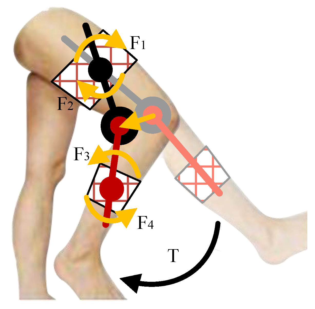
Due to the non-rigid nature of human tissue, each limb of the human body can be regarded as a rotating body. In order to transmit the force or torque of the exoskeleton to the limb, the human–machine interface connection needs to be wrapped around the thigh and calf segments. These connecting components convert the force or torque exerted by the exoskeleton into pressure acting on the surface of the skin. Therefore, it is necessary to avoid intense stress at the connection. As shown in Figure 8, the motion compatibility of the knee joint exoskeleton with a single degree of freedom rotation was analyzed with a driving torque of T and a binding force of F n ( n = 1 , 2 , , n ) on the human body. When the joints in the human–machine interface do not match, it is reflected in the inconsistent instantaneous center of the human–machine movement, and the binding will show a trend of movement and deformation. Thus, the assistance will be dispersed in the deformation of the binding, thereby affecting the fit between the exoskeleton and the human body and greatly reducing the assistance performance of the exoskeleton [23].
During exercise, the lower limbs have a considerable amplitude of motion. So, if the exoskeleton is installed far from the center of mass of the human body, it may bring additional metabolic costs to the wearer. Based on this consideration, we proposed installing the exoskeleton near the centroid of the user’s thighs and shanks to minimize potential additional metabolic costs. As shown in Figure 9, six preliminary configurations of knee exoskeleton mechanisms were proposed, with knee exoskeletons connected to the centroid positions of the thighs and shanks, represented as COM t and COM s , respectively. The thigh strap of the exoskeleton was fixed near the center of mass of the thigh, and the knee joint adopted a single-hinge (SH) and a cross-four-link (FBL) structure, respectively. The lower leg connection used a moving pair (P) or ball joint (S) connection method. This lays a theoretical foundation for selecting a configuration for an assisted exoskeleton mechanism that is similar in function to the human knee joint.

3. Kinematics and Dynamics Model of Lower Limbs

3.1. Manikin Simplification

Using a large number of human biomechanical experiments, it has been shown that human lower limb movements mostly occur in the sagittal plane. Due to the fact that the design of wearable exoskeleton devices basically meets human motion requirements, in order to facilitate calculation, the lower limb assistance device can be simplified to a series link model. The lower limb passive assistance device designed above mainly covers the human hip and knee joints, excluding the foot and ankle regions. Therefore, a simplified link model was established by simplifying the foot effect. During the modeling process, the human body was divided into 15 parts, including the head, upper torso, two upper arms, two forearms, two hands, lower torso, two thighs, two legs, and two feet. This paper mainly studies the characteristics of lower limb kinematics and dynamics, thus the person’s upper arm, forearm, and hand were combined into a single part called the upper body, while the head was ignored in modeling. In this paper, only the motion in the sagittal plane was considered, and the model for the human–machine system was simplified to obtain a connecting rod model, as shown in Figure 5. In the sagittal plane, each part of the human body’s upper limbs, left and right thighs, left and right shanks, and left and right feet can be regarded as seven connected bones, ignoring the influence of muscles on motion, thereby simplifying the seven-link simplified model of the human body.
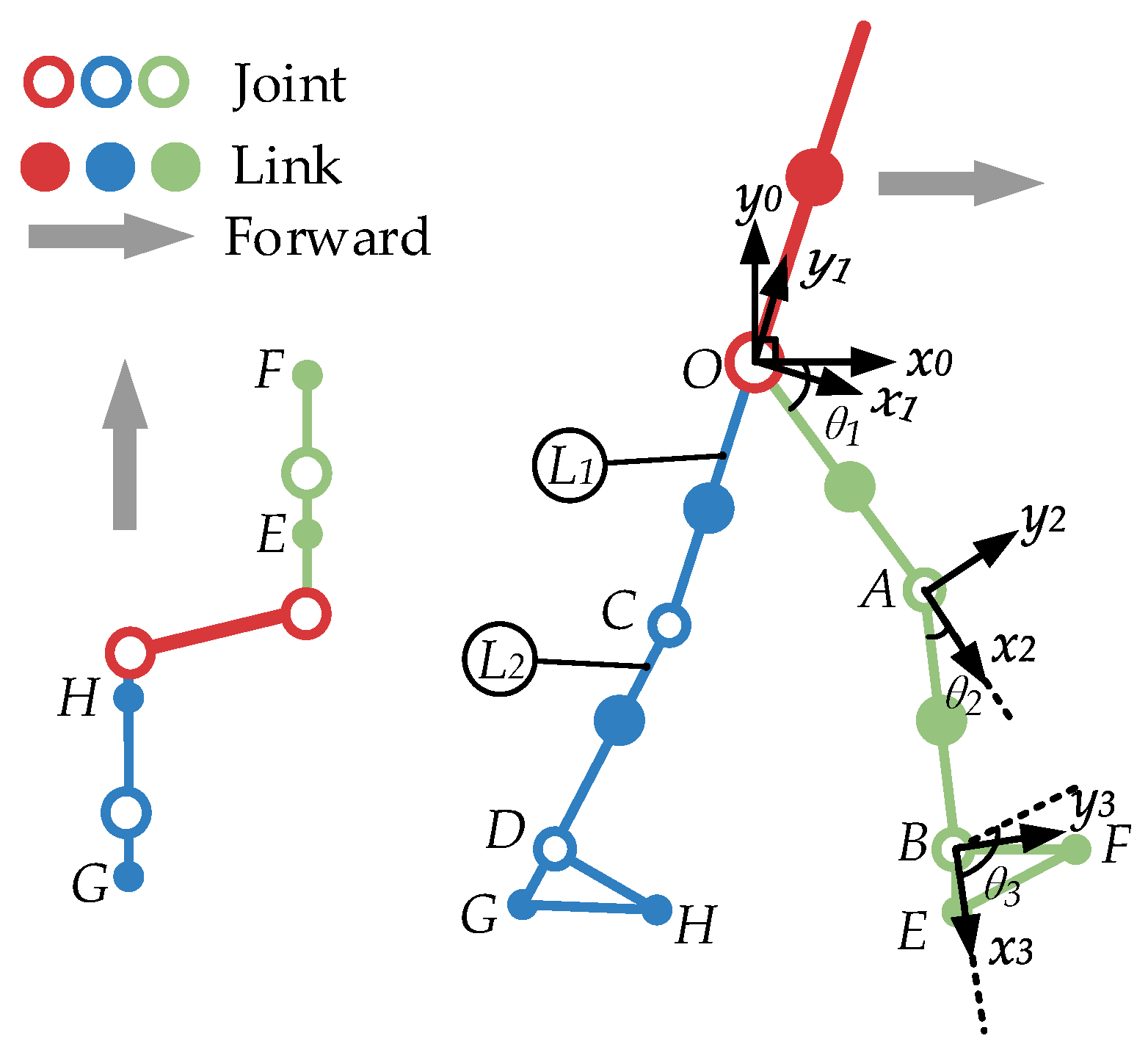
The establishment of the kinematics model for the passive lower limb assistance device can determine the relevant kinematics equations using mathematical tools, such as matrices and vectors. In general, the kinematics model of the lower limb assistance device mainly establishes the relationship between the motion trajectory, angle, angular velocity, and other variables of the end effector in the reference coordinate system and time. Because the lower limb joints are mostly considered rigid body systems during kinematic analysis, the D-H method for establishing traditional robot kinematic models was used to establish the kinematic model of the lower limb assist device [24,25]. The established D-H kinematics model and the definition of reference coordinate systems, local coordinate systems, and related parameters are shown in Figure 10.
In Figure 10, point O represents the hip joint, points C and A represent the left and right knee joints, respectively, points D and B represent the ends of the left and right lower limbs, respectively, points G and E represent the heel points of the left and right feet, respectively, and points H and F represent the toe points of the left and right feet, respectively. The thigh length of the left and right legs is L 1 , and the shank length of the left and right legs is L 2 . θ 1 is the included angle between connecting rod L 1 in the horizontal direction and θ 2 is the included angle between connecting rod L 1 and connecting rod L 2 , which is positive in the counterclockwise direction.
According to the D-H model established based on the above, because there is only a single free change in the sagittal plane, the exoskeleton device does not undergo joint torsional motion or joint translational motion along the sagittal axis in the sagittal plane. The relevant parameter settings are shown in Table 3.
In Table 3, L i is the i th member, α i is the joint torsion angle, a i is the member length, d i is the joint translation amount, and θ i is the joint angle change. In the same plane, α i = 0 , d i = 0 , a 2 = L 1 , and a 3 = L 2 . T i i 1 represents the transformation matrix from coordinate system i 1 to i . According to the parameter content shown in Table 3, the transformation matrix T i i 1 at the coordinate of point i relative to point i 1 is established as:
T i i 1 = [ cos ( θ i ) sin ( θ i ) cos ( α i ) sin ( θ i ) sin ( α i ) a i cos ( θ i ) sin ( θ i ) cos ( θ i ) cos ( α i ) cos ( θ i ) sin ( α i ) a i sin ( θ i ) 0 sin ( α i ) cos ( α i ) d i 0 0 0 1 ]
The final transformation matrix is:
T i 0 = T 1 0 T 2 1 T i i 1

3.2. Kinematic Model of Human Lower Limbs

According to the D-H (Denavit–Hartenberg) method in robot kinematics [24], forward and inverse kinematics models of human lower limbs are established. Using the right leg of a human lower limb as an example, a coordinate system is established at each joint. The origin of the coordinate system is O ( x 0 , y 0 , z 0 ) , the moving coordinate system of the right hip joint is ( x 1 , y 1 , z 1 ), the moving coordinate system of the knee joint is ( x 2 , y 2 , z 2 ), and the moving coordinate system of the ankle joint is ( x 3 , y 3 , z 3 ). The simplified model of the exoskeleton human–machine system is shown in Figure 10. Among them, both the hip and ankle joints have 3 degrees of freedom (roll, pitch, and yaw), and the knee joint has 1 degree of pitch freedom, a total of 7 degrees of freedom, and 14 generalized coordinates.
The research in this article aims to establish a coordinate system for the movement of a single lower limb. The homogeneous coordinate change matrix between each connecting rod is:
T 1 0 = [ cos ( θ 1 ) sin ( θ 1 ) 0 0 sin ( θ 1 ) cos ( θ 1 ) 0 0 0 0 1 0 0 0 0 1 ]
T 2 1 = [ cos ( θ 2 ) sin ( θ 2 ) 0 L 1 sin ( θ 2 ) cos ( θ 2 ) 0 0 0 0 1 0 0 0 0 1 ]
T 3 2 = [ cos ( θ 3 ) sin ( θ 3 ) 0 L 2 sin ( θ 3 ) cos ( θ 3 ) 0 0 0 0 1 0 0 0 0 1 ]
T 3 0 = [ cos ( θ 1 + θ 2 + θ 3 ) sin ( θ 1 + θ 2 + θ 3 ) 0 L 1 cos ( θ 1 ) + L 2 cos ( θ 1 + θ 2 ) sin ( θ 1 + θ 2 + θ 3 ) cos ( θ 1 + θ 2 + θ 3 ) 0 L 2 sin ( θ 1 + θ 2 ) + L 1 sin ( θ 1 ) 0 0 1 0 0 0 0 1 ]
The forward kinematics solution is defined as obtaining the position and posture of the end effector relative to the reference coordinate system by knowing the motion parameters of each joint. The inverse solution is defined as calculating the motion parameters for each joint based on the position and posture of the end effector relative to the reference coordinate system that meets the working requirements. The direction of solving the forward and inverse kinematics solutions is opposite. Combining the VICON motion capture data, the spatial position coordinates of the marker point are obtained, and the spatial position and posture coordinates P = ( p x , p y ) of the terminal in the absolute coordinate system are calculated as follows:
{ p x = L 1 cos ( θ 1 ) + L 2 cos ( θ 1 + θ 2 ) p y = L 2 sin ( θ 1 + θ 2 ) + L 1 sin ( θ 1 )
where p x is the relationship between step height and joint angle and p y is the relationship between step length and joint angle.
Equations (20)–(24) are forward kinematics formulas for the lower limbs of the human body. The step length and step height are obtained using known changes in the joint angle. Inverse kinematics involves solving six joint angles based on the transformation matrix T obtained above. There are analytical, geometric, and iterative methods for solving inverse kinematics. Analytical methods are used here. Using motion capture technology to obtain the position coordinates of spatial marker points, and solving Equations (20)–(24), the solutions for θ 1 and θ 2 can be obtained as follows:
{ θ 1 = arctan ( y 3 x 3 ) ± arccos ( x 3 2 + y 3 2 + L 1 2 L 2 2 2 L 1 x 3 2 + y 3 2 ) θ 2 = ± arccos ( x 3 2 + y 3 2 L 1 2 L 2 2 2 L 1 L 2 )
Therefore, the hip joint angle θ h and the knee joint angle θ k can be expressed as:
{ θ h = θ 1 × 180 ° π + 90 ° θ k = θ 2 × 180 ° π
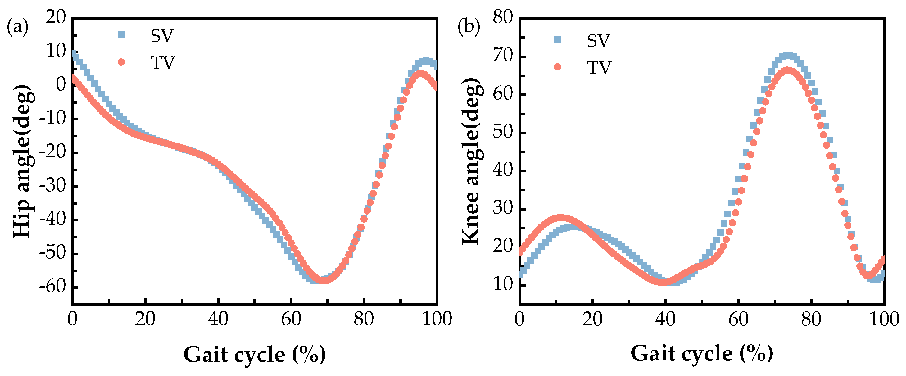
Based on the above forward and inverse kinematics mathematical models, using MATLAB software for modeling and analysis, a theoretical curve of angle change within the motion cycle of the hip and knee joints was obtained, as shown in Figure 11. The red curve represents the theoretical-calculated value (TV), and the blue curve represents the simulation software-calculated value (SV).
The TV curve in Figure 11 was obtained with mathematical modeling and simulation analysis using MATLAB. The SV curves were obtained by analyzing and simulating 3D motion capture data using the spatial coordinates of marker points in Visual3D biomechanical analysis software. Using a comparison, it can be seen that the obtained knee joint angle variation law is basically consistent with the standard curve variation law. However, due to measurement error in the leg length input parameter, there are certain differences between the lowest and highest angle values. The correctness of the mathematical model was verified using simulation.

3.3. Man–Machine System Dynamics Model

In the exoskeleton robot system, it is necessary to conduct relevant dynamics research to study the auxiliary effects of wearing an exoskeleton during human motion. Among the methods, dynamic analysis is mainly divided into two aspects, which include positive dynamics and inverse dynamics. Inverse dynamics refers to calculating the torque generated by joint motion using the angle, velocity, and acceleration of each joint of the lower limb. On the contrary, forward dynamics refers to calculating the angle, angular velocity, and angular acceleration of joint motion using the torque generated by joint motion. To study the dynamics of the human lower limb-assisted exoskeleton, it is necessary to establish the torque and joint motion information parameters generated when wearing the exoskeleton. By establishing a simplified link model, the system dynamics problem is transformed into a problem between the motion of the link and the torque of the link. To simplify the complexity of the system, a dynamic mathematical model of an exoskeleton robot was established. Solving the driving torque of the knee joint will provide a theoretical reference for solving the dynamic parameters in the motion process.
At present, the common dynamics analysis methods include the general theorem of dynamics, the Newton–Euler method [26], the Lagrange formula [27], the Kane method, and the Robertson–Wittenburg method. The two main theoretical methods for analyzing the system dynamics model are the Lagrange kinematics method and the Newton–Euler motion method. Among them, the Lagrange method obtains the generalized external forces and moments of the system by establishing a differential equation for the difference between kinetic energy and potential energy. There is no constraint reaction in the Lagrange equation, and the solving process is independent of the selection of generalized coordinates. Therefore, this article uses the Lagrange method to analyze the dynamic characteristics of the human lower limbs. The Lagrange formula was used, and the Lagrange function L was defined as the difference between the system kinetic energy K and the potential energy P, i.e.,
L = K P
In the simplified link model, the total kinetic energy K and the total potential energy P of the upper and lower legs are as follows:
{ K = 1 2 [ ( m 1 + m 2 ) θ ˙ 1 2 l 1 2 + m 2 l 2 2 ( θ ˙ 1 θ ˙ 2 ) 2 ] + m 2 l 1 l 2 cos ( θ 2 ) ( θ ˙ 1 θ ˙ 2 ) θ ˙ 1 + 1 2 ( I 1 θ ˙ 1 2 + I 2 θ ˙ 2 2 ) P = ( m 1 + m 2 ) g l 1 ( 1 cos θ 1 ) + m 2 g l 2 [ 1 cos ( θ 1 θ 2 ) ]
where the masses of the big and small legs are m 1 and m 2 , respectively. The lengths of the big and small legs are l 1 and l 2 , respectively. The moment of inertia for the big and small legs are I 1 and I 2 , respectively. The generalized coordinate of the angle is θ i . The acceleration of gravity is g . The Lagrange function obtained by substituting Equation (28) into Equation (27) is as follows:
L = 1 2 [ ( m 1 + m 2 ) θ 1 ˙ 2 l 1 2 + m 2 l 2 2 ( θ 1 ˙ θ 2 ˙ ) 2 ] + 1 2 [ I 1 θ 1 ˙ 2 + I 2 θ 2 ˙ 2 ] + m 2 l 1 l 2 cos θ 2 ( θ 1 ˙ θ 2 ˙ ) θ 1 ˙ ( m 1 + m 2 ) g l 1 ( 1 cos θ 1 ) m 2 g l 2 [ 1 cos ( θ 1 θ 2 ) ]
The general form of the dynamic equation is as follows:
T i = d d t ( L θ ˙ i ) L θ i , ( i = 1 , 2 , , n )
where n is the degree of freedom of the system and θ ˙ i is the speed. θ i is the generalized coordinate, which represents the joint coordinates of kinetic energy K and potential energy P . T i is the force/moment in the generalized coordinates, where it represents the force/moment acting on the i -th coordinate. By substituting the model parameters into Equation (30), the dynamic equation can be described using a second-order nonlinear differential equation:
τ = M ( q ) q ¨ + C ( q , q ˙ ) q ˙ + G ( q )
where q , q , ˙ and q ¨ are, respectively, the generalized coordinates, generalized velocities, and generalized accelerations of the connecting rod model. M ( q ) is the inertial force matrix of the connecting rod, which is affected by angular acceleration. C ( q , q ˙ ) is the torque caused by Coriolis force and centripetal force. G ( q ) is the gravity matrix of the connecting rod, and τ is the generalized torque of the connecting rod.
The detailed expressions for these coefficients can be found in Equations (32)–(37).
τ = [ T 1 T 2 ]
q ˙ = [ θ 1 ˙ θ 2 ˙ ]
q ¨ = [ θ 1 ¨ θ 2 ¨ ]
M = [ m 1 l 1 2 + m 2 l 1 2 + m 2 l 2 2 + 2 m 2 l 1 l 2 cos θ 2 + I 1 m 2 l 2 2 m 2 l 1 l 2 cos θ 2 m 2 l 2 2 m 2 l 1 l 2 cos θ 2 ( m 2 l 2 2 + I 2 ) ]
C = [ 0 2 m 2 l 1 l 2 sin θ 2 θ 1 ˙ + m 2 l 1 l 2 sin θ 2 θ 2 ˙ m 2 l 1 l 2 sin θ 2 θ 1 ˙ 0 ]
G = [ ( m 1 + m 2 ) g l 1 sin θ 1 + m 2 g l 2 sin ( θ 1 θ 2 ) m 2 g l 2 sin ( θ 1 θ 2 ) ]
Therefore, the expressions for the hip and knee moment T 1 and T 2 are as follows:
T 1 = ( m 1 l 1 2 + m 2 l 1 2 + m 2 l 2 2 + 2 m 2 l 1 l 2 cos θ 2 + I 1 ) θ 1 ¨ + ( m 2 l 2 2 m 2 l 1 l 2 cos θ 2 ) θ 2 ¨ 2 m 2 l 1 l 2 sin θ 2 θ 1 ˙ θ 2 ˙ + m 2 l 1 l 2 sin θ 2 θ 2 ˙ 2 + ( m 1 + m 2 ) g l 1 sin θ 1 + m 2 g l 2 sin ( θ 1 + θ 2 )
T 2 = ( m 2 l 2 2 + m 2 l 1 l 2 cos θ 2 ) θ 1 ¨ + ( m 2 l 2 2 + I 2 ) θ 2 ¨ + m 2 l 1 l 2 sin θ 2 θ 1 ˙ 2 m 2 g l 2 sin ( θ 1 + θ 2 )

4. Human Machine Coupling Simulation Experiment

4.1. Establishment of a Three-Dimensional Human Body Model

In order to improve simulation efficiency, Adams software was used to simulate human walking, which simplified the human body model to a certain extent. A male with a height of 1.8 m and a mass of 75 kg was selected as the research object. Considering the complexity of the human body structure, based on research accuracy and research needs, the human body can be abstracted and simplified, and various parts of the human body can be abstracted into simple rigid geometric entities.
A simplified model of the human body was established using Solidworks software, and the human body was divided into 14 individual segments, including the head and neck, torso, left and right upper arms, left and right forearms, left and right hands, left and right thighs, left and right shanks, and left and right feet. The model was imported into Adams dynamic simulation software using the Parasolid format, as shown in Figure 12.
The inertia parameters of the human body model were determined according to GB/T 17245-2004 “Inertia Parameters of Adult Human Body”. A binary regression equation was used to calculate the individual inertia parameters of the simulation model, and the regression equation is as follows:
Y = B 0 + B 1 X 1 + B 2 X 2
where B 0 , B 1 , and B 2 are coefficients in the regression equation, X 1 is the body mass of the human body, and X 2 is the height of the human body. The detailed parameters involved in the lower limb regression equation are listed in Table 4.
The specific parameters for each body segment calculated using Equation (31) are shown in Table 5. The starting points for measuring the centroid position were the vertex of the head, cervical spine, perineal point, acromion point, radial point, radial styloid process point, middle fingertip point, tibial point, inner ankle point, and plantar area.
After the models for each body segment were established, they were assembled and verified according to the actual human body structure to eliminate dimensional errors. In addition, due to the simulation of walking on flat ground, a ground model was established.

4.2. Applying Constraints

Based on the actual relative motion of each human body segment, a simulation model was constructed and constraints (joints) were added. The main focus of this article is on the movement of the lower limbs. thus, we connected the head, neck, and torso segments together in the form of fixed pairs and added rotating pairs to the arms. The relative motion between the trunk and thighs is rotational, so a rotational pair was added between the trunk and thighs to simulate hip joint motion. Similarly, a rotation pair was added between the thighs and shanks. A rotation pair was added between the shanks and feet to simulate the rotational motion of the knee and ankle joints. During the walking experiment, the ground model was fixed, so a fixed pair was added between the floor and the ground. Since only the movement of the human body in the sagittal plane was studied, parallel constraints were added between the human body and the ground model. This prevented the human body simulation model from tilting left and right during movement.

4.3. Applying Drive and Contact

After adding each constraint, it was necessary to add appropriate motion and contacts to enable the model to achieve the expected motion. The driving forms of the motion pair in ADAMS software mainly include translational driving and rotational driving, and various physical quantities can be used as a driving form. Translational motion can be driven by physical quantities such as displacement and velocity of the object. The motion form of rotation is driven by physical quantities such as angle and angular velocity. In addition, it can also be driven by physical quantities such as force and torque.
The driving form used in this article was determined by adding rotational drives to the rotation pairs of each joint in the lower limb and importing the angle curves for each joint obtained from the previous section into ADAMS to generate spline curves (splines) as driving variables. The AKISPL function was selected as the driver function type, and its basic form was AKISPL (1st_Indep_Var, 2nd_Indep_Var, Spline_Name, Deriv_Order). Among them, 1st_Indep_Var is the first independent variable of the spline curve, and since the angle curve used reflects the change in angle with respect to time, it is set to time; 2nd_Indep_Var is the second independent variable of the spline, which is set to 0; Spline_Name is the name of the spline curve used, which is set to the corresponding angle curve name; and Deriv_Order is the differential order of the interpolation point, which is set to 0. The above steps were repeated to sequentially set the six joint drive settings for both legs.
Finally, the walking simulation also needed the contact form to be set between the foot and the ground, which was implemented using the contact function in ADAMS. The contact effect was set between the foot and the ground, and the contact type was rigid body to rigid body. The various parameter settings are shown in Table 6. In the simulation experiment, the termination time was set to 3.65 s, the simulation step size was set to 0.02, and the default settings were used for the rest.

4.4. Simulation and Post-Processing Analysis

After the above settings were completed, the simulation started with dynamics selected as the analysis type. This article uses flat road conditions as an example for analysis, and it can be seen that the established model can walk smoothly and steadily. Using the measurement function in ADAMS software, the torque of each joint in the lower limb of the model was measured. A comparison of the measured joint torques with the calculated joint torques is shown in Figure 13.
By comparing the joint torques obtained from the ADAMS simulation and the joint torques calculated using the mathematical model, the similarity between the two curves was determined. This article used the method of statistical complex correlation coefficient as an evaluation indicator to describe the similarity between the two curves. The correlation coefficient was first calculated, and then the effectiveness test was conducted. The formula for calculating the complex correlation coefficient is as follows [29]:
R = 1 i = 1 m j = 1 n ( x i j x ¯ j ) 2 / n ( m 1 ) i = 1 m j = 1 n ( x i j x ¯ ) 2 / ( n m 1 )
where m represents the number of curves, n represents the amount of data in each curve, x i j represents the jth value of the i-th curve, x ¯ j represents the average value of the jth data on the m-th curve, and x ¯ represents the average value of n data on the m-th curve. The closer the complex correlation coefficient R is to 1, the higher the correlation between the two curves, and vice versa. The polyphase relationship numbers R between the simulated results from the hip and knee joint experiments and the mathematical model results obtained using SPSS data statistical analysis software were 0.850 and 0.873, respectively, with a significance level p < 0.001. This indicates that the correlation between the torque curves for each joint calculated using the mathematical model and simulation model established in this study reached a very significant level.

4.5. Wearing Exoskeleton Simulation Results

Based on human motion simulation, the exoskeleton was connected to the lower limbs of the human body according to the preliminary six knee joint mechanism configurations. The exoskeleton machine is mainly made of aluminum alloy material, with a density of 2.74 × 10⁻⁶ kg/mm3, a Young’ s modulus of 7.1705 × 10⁴ n/mm2, and a Poisson’s ratio of 0.33. The thigh and shank straps are constrained to the human body with a sleeve force. The translation characteristics on the x, y, and z components were all set to 25 n/mm, and the damping was set to 0.25 n s/mm. The rotational characteristics on the x, y, and z components were all set to 1.4137166941 n mm/deg, and the damping was set to 0.3490658504 n mm s/deg. In order to avoid the impact of different qualities on the results, all simulation results underwent quality normalization.
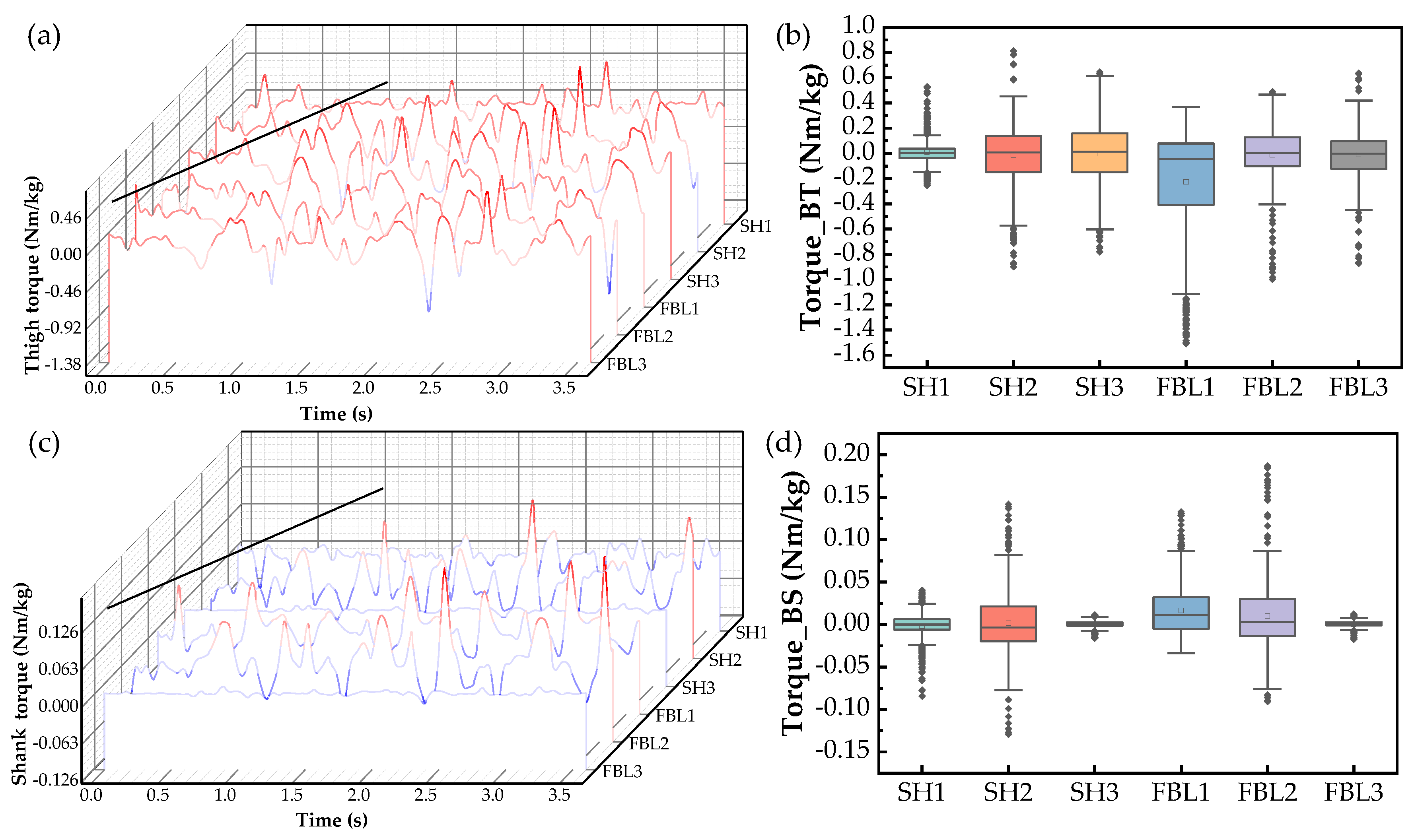
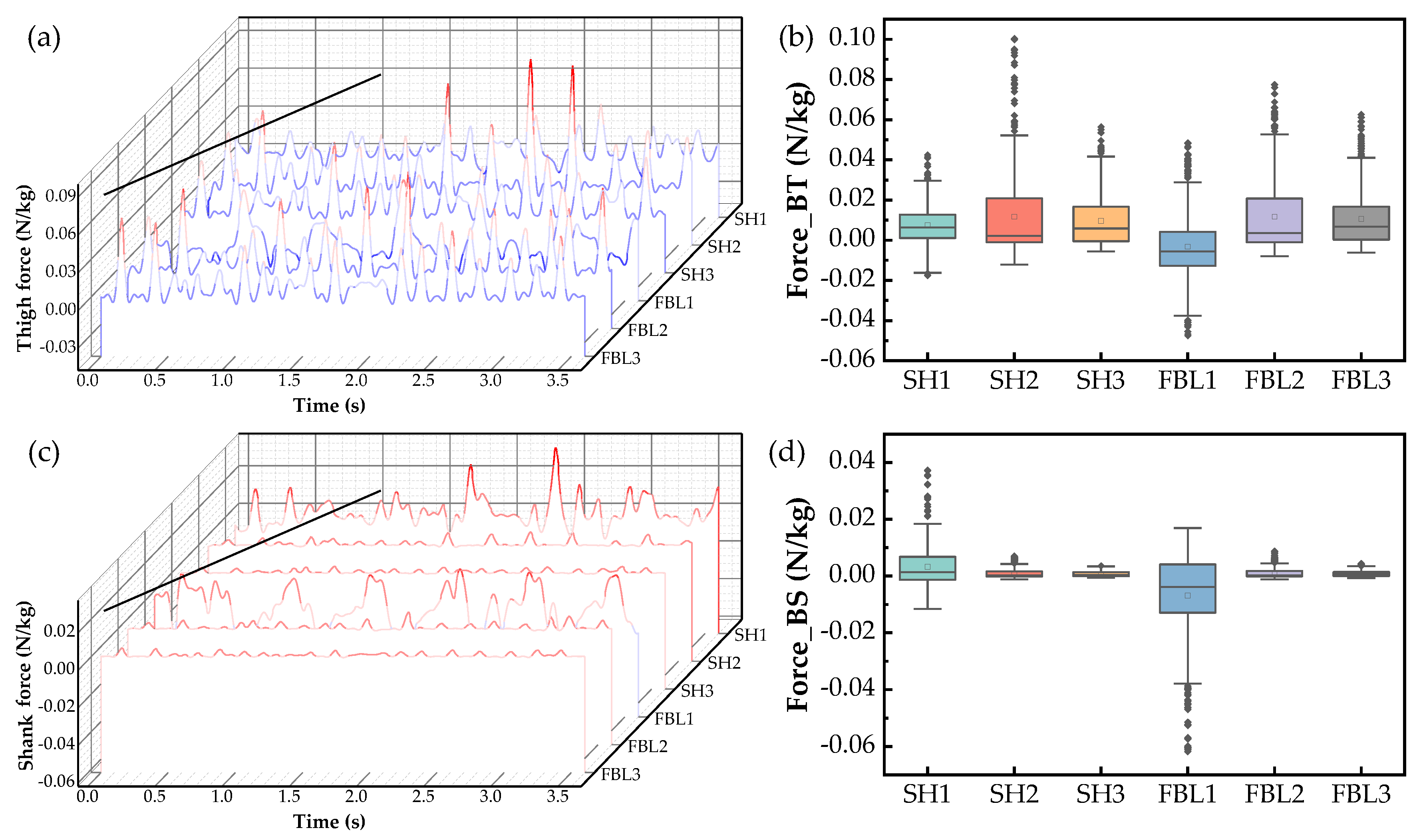
Considering the large and small legs of the human body as cylinders, we analyzed the radial torque generated around the legs, as well as the changes in axial force along the direction of the limbs. After wearing the knee joint exoskeleton simulation, the radial torque changes at the human–machine connection were obtained. As shown in Figure 14a,c, the torque changes in the thigh and shank over time were characterized, with red representing positive values and blue representing negative values. As shown in Figure 14b,d, the box plot for the data from this scheme over a period of time reflects the average, median, and fluctuation in the group data. The axial force changes along the leg at the fixed positions of the thigh and shank in the knee joint exoskeleton are shown in Figure 15a–c.
By calculating the mean, median, range and quartile spacing for each group of simulation data, the concentration of torque and force were obtained. The comfortable wearing effect should be to reduce the emergence of sudden torque and force. As shown in Figure 13 and Figure 14 and Table 7, the wearing results for the six mechanism configurations show that the torque and force at the thigh connection were much greater than those at the shank connection. The reason for this result is due to the mismatch between the device’s weight and wearing, which generates an external force. The thigh joint bears a large amount of inertial force during the movement process, which disperses most of the external force brought about by wearing the exoskeleton. From the changes in radial torsion of the thigh straps, it was found that the average values of thigh torque for the SH3 and FBL3 schemes were 15.1 × 10 4   Nm / kg and 95.4 × 10 4   Nm / kg , respectively. The average values of shank torque were 5.0 × 10 4 Nm / kg and 5.4 × 10 4   Nm / kg , respectively. All the values were lower than other configuration schemes within the group. Due to the use of rotating pairs in the driving of the human body simulation model, the SH3 mechanism had better human–machine compatibility compared to the FBL3 mechanism. From the changes in the axial force of the thigh strap, it was found that the SH1 and FBL1 schemes had the smallest force on the thigh ( 74.5 × 10 4   N / kg and 32.8 × 10 4   N / kg , respectively), while the shank had the highest force level within the group (32.3 ×   10 4   N / kg and −68.9 ×   10 4   N / kg , respectively). The force on the lower legs of the SH3 and FBL3 schemes was the smallest within the group (7.5 ×   10 4   N / kg and 8.5 ×   10 4   N / kg , respectively), while the force on the thighs was moderate within the group (96 N/kg and 105.4 N/kg, respectively). Additionally, in the SH3 and FBL3 schemes, the torque and force on the lower leg were more concentrated, and no extreme data appeared. Therefore, the SH3 and FBL3 schemes are the more preferred options.
It must be highlighted that (1) the simulation model only considers multiple rigid bodies, without considering muscles, tendons, ligaments, etc., and further in-depth research will be conducted in the later stage and (2) the corresponding simulation results need to be further verified by processing a prototype using experiments. In addition, to be sure that the protocol is universal, more subjects should be included representing both sexes, various physical conditions, and body shapes. So, these limitations will be considered seriously in our future research.

5. Conclusions

Using spatiotemporal data on human walking gait, a simplified mathematical model of lower limbs was established, and the mathematical models of kinematics and dynamics were simulated and verified. Based on the macro- and micro-motion mechanisms of the knee joint, a design scheme for the exoskeleton mechanism of the knee joint was proposed. The human–machine model was analyzed using Adams dynamics simulation software, and the kinematics and dynamics data were obtained under the wearing motion state. The radial torque and axial force imposed by the exoskeleton on the leg were mainly selected for analysis. The simulation results indicated that the SH3 and FBL3 schemes are the preferred options. Considering that the actual physiological movement of the knee joint is variable axis rotation, choosing the FBL3 scheme is better. The optimized exoskeleton configuration of the knee joint was verified to be more in line with human knee joint motion, and the exoskeleton gait is more in line with human gait.

Author Contributions

Conceptualization, X.T. and X.W.; methodology, X.T. and Y.X.; software, X.T.; validation, X.T., R.Y. and J.Y.; formal analysis, X.W.; investigation, R.Y.; resources, X.T.; data curation, X.T.; writing—original draft preparation, X.T.; writing—review and editing, X.W. and Y.X.; visualization, X.T.; supervision, X.W.; project administration, X.W.; funding acquisition, X.W. All authors have read and agreed to the published version of the manuscript.

Funding

This work was supported by the Ministry of Education Youth Fund Project (grant number 21XJC760003), the Outstanding Talents Support Program Project (grant number 106-451420001), and the Common technology and field fund for equipment pre research (grant numbers 106-418321001). The authors would like to express their appreciation to these agencies.

Institutional Review Board Statement

The study was conducted in accordance with the Declaration of Helsinki, and approved by the Institutional Review Board (or Ethics Committee) of Medical Ethics Committee of Children’s Hospital Affiliated to Xi’an Jiaotong University (Scientific ethics review number: 20230301-16).

Informed Consent Statement

Informed consent was obtained from all subjects involved in the study.

Data Availability Statement

The data presented in this study are available on request from the corresponding author.

Conflicts of Interest

The authors declare no conflict of interest.

References

  1. Weber, W.; Weber, E. Mechanik Der Menschlichen Gehwerkzeuge; Göttingen, Germany, 1836; pp. 1–496. [Google Scholar]
  2. Bresler, B.; Frankel, J. The Forces and Moments in the Leg During Level Walking. J. Appl. Mech. 1950, 72, 27–36. [Google Scholar] [CrossRef]
  3. Hao, Z.X.; Leng, H.J.; Qu, C.Y.; Wan, C. Biomechanics of the Bone and the Joint. J. Solid Mech. 2010, 31, 603–612. [Google Scholar]
  4. Fuge, A.; Herron, C.; Beiter, B.; Kalita, B.; Leonessa, A. Design, development, and analysis of the lower body of next-generation 3D-printed humanoid research platform: PANDORA. Robotica 2023, 41, 2177–2206. [Google Scholar] [CrossRef]
  5. Sun, Z.; Li, Y.; Zi, B.; Chen, B. Design, Modeling, and Evaluation of a Hybrid Driven Knee-Ankle Orthosis With Shape Memory Alloy Actuators. ASME J. Mech. Des. 2023, 145, 063301. [Google Scholar] [CrossRef]
  6. Sulzer, J.S.; Roiz, R.A.; Peshkin, M.A.; Patton, J.L. A Highly Back Drivable, Lightweight Knee Actuator for Investigating Gait in Stroke. IEEE Trans. Robot. 2009, 25, 539–548. [Google Scholar] [CrossRef] [PubMed] [Green Version]
  7. Chaichaowarat, R.; Kinugawa, J.; Kosuge, K. Unpowered Knee Exoskeleton Reduces Quadriceps Activity during Cycling. Engineering 2018, 4, 471–478. [Google Scholar] [CrossRef]
  8. Wang, D.; Lee, K.M.; Guo, J.J.; Yang, C.J. Adaptive Knee Joint Exoskeleton Based on Biological Geometries. IEEE/ASME Trans. Mechatron. 2014, 19, 1268–1278. [Google Scholar] [CrossRef]
  9. Douglas, A.D.; Mohamed, R.M.; Richard, D.K.; William, H. In Vivo Determination of Normal and Anterior Cruciate Ligament-Deficient Knee Kinematics. J. Biomech. 2005, 38, 241–253. [Google Scholar]
  10. Van Den Bogert, A.J.; Reinschmidt, C.; Lundberg, A. Helical Axes of Skeletal Knee Joint Motion during Running. J. Biomech. 2008, 41, 1632–1638. [Google Scholar] [CrossRef] [Green Version]
  11. Wolf, A. Instantaneous Screws of Weight-Bearing Knee: What Can the Screws Tell Us About the Knee Motion. J. Biomech. Eng. 2014, 136, 433–440. [Google Scholar] [CrossRef] [Green Version]
  12. Chen, J.T.; Yang, L.F.; Wang, Y.X.; Long, Q. The New Simulated Knee Prosthesis of Discontinuity Instantaneous Center Curve. Mach. Des. Manuf. 2014, 281, 183–185. [Google Scholar]
  13. Choi, B.; Lee, Y.; Kim, J.; Lee, M.; Lee, J.; Roh, S.G.; Choi, H.; Kim, Y.-J.; Choi, J.-Y. A Self-aligning Knee Joint for Walking Assistance Devices. In Proceedings of the 2016 38th Annual International Conference of the IEEE Engineering in Medicine and Biology Society (EMBC), Orlando, FL, USA, 16–20 August 2016; IEEE: Orlando, FL, USA, 2016; pp. 2222–2227. [Google Scholar]
  14. Zhang, L.; Liu, G.; Han, B.; Wang, Z.; Li, H.; Jiao, Y. Assistive devices of human knee joint: A review. Robot. Auton. Syst. 2020, 125, 103394. [Google Scholar] [CrossRef]
  15. Jiang, J.; Chen, P.; Peng, J.; Qiao, X.; Zhu, F.; Zhong, J. Design and Optimization of Lower Limb Rehabilitation Exoskeleton with a Multiaxial Knee Joint. Biomimetics 2023, 8, 156. [Google Scholar] [CrossRef] [PubMed]
  16. Shin, Y.J.; Kim, G.T.; Kim, Y. Optimal Design of Multi-linked Knee Joint for Lower Limb Wearable Robot. Int. J. Precis. Eng. Manuf. 2023, 24, 967–976. [Google Scholar] [CrossRef]
  17. Shuai, Y.M.; Xu, Z.; Li, S.Z.; Liu, X.H. Selection and Optimization of Multicentre Extremity Knee-Mechanism. J. Jianghan Pet. Inst. 2001, 23, 86–88. [Google Scholar]
  18. Bertomeu, J.M.; Lois, J.M.; Guillem, R.B.; Pozo, A.P.; Lacuesta, J.; Mollà, C.G.; Luna, P.; Vera, P.; Jaime, P. Development of a Hinge Compatible with the Kinematics of the Knee Joint. Prosthet. Orthot. Int. 2007, 31, 371–383. [Google Scholar] [CrossRef] [Green Version]
  19. Walker, P.S.; Kurosawa, H.; Rovick, J.S.; Zimmerman, R.A. External Knee Joint Design Based on Normal Motion. J. Rehabil. Res. Dev. 1985, 22, 9–22. [Google Scholar] [CrossRef]
  20. Jarrasse, N.; Morel, G. Connecting a Human Limb to an Exoskeleton. IEEE Trans. Robot. 2013, 28, 697–709. [Google Scholar] [CrossRef] [Green Version]
  21. Zhang, J.L. Design and Kinematic Analysis of Double Motor Driven Hexapod Upright Walking Mechanism. J. Mech. Transm. 2012, 42, 106–111. [Google Scholar]
  22. Denavit, J.; Hartenberg, R.S. Closure to “Discussions of ‘Approximate Synthesis of Spatial Linkages’”. ASME J. Appl. Mech. 1960, 27, 757–758. [Google Scholar]
  23. Bagheri, M.; Naseradinmousavi, P. Analytical and Experimental Nonzero-Sum Differential Game-Based Control of A 7-Dof Robotic Manipulator. J. Vib. Control 2022, 28, 707–718. [Google Scholar] [CrossRef]
  24. Li, X.; Sun, H.X.; Liao, L.J.; Song, J. Simulation and Comparison Research of Lagrange and Kane Dynamics Modeling for the 4-Dof Modular Industrial Robot. In Proceedings of the 5th International Conference on Advanced Design and Manufacturing Engineering, Shenzhen, China, 19–20 September 2015; Atlantis Press: Shenzhen, China, 2015. [Google Scholar]
  25. Gao, M.; Wang, Z.; Pang, Z.; Sun, J.; Li, J.; Li, S.; Zhang, H. Electrically Driven Lower Limb Exoskeleton Rehabilitation Robot Based on Anthropomorphic Design. Machines 2022, 10, 266. [Google Scholar] [CrossRef]
  26. Yu, C.; Yao, K.; Zong, Y.; Ye, J.; Chen, J. Rigid-Body Guidance Synthesis of Noncircular Gear-Five-Bar Mechanisms and Its Application in a Knee Joint Rehabilitation Device. Machines 2022, 10, 1110. [Google Scholar] [CrossRef]
  27. Shafiei, M.; Behzadipour, S. Adding Backlash to the Connection Elements can Improve the Performance of a Robotic Exoskeleton. Mech. Mach. Theory 2020, 152, 103937. [Google Scholar] [CrossRef]
  28. Zhang, Y.; Zhang, H.M.; Xuan, B.K.; Zhang, Y.C. Motion Analysis and Simulation of Lower Limb based on ADAMS. J. Syst. Simul. 2017, 29, 988–995. [Google Scholar]
  29. Li, X.H.; Hao, W.Y.; Xiao, X.F.; Wu, C.L. Simulation and Validation of Human Model in Landings Based on ADAMS. LifeMoD. Zhejiang Sport Sci. 2015, 37, 114–116. [Google Scholar]
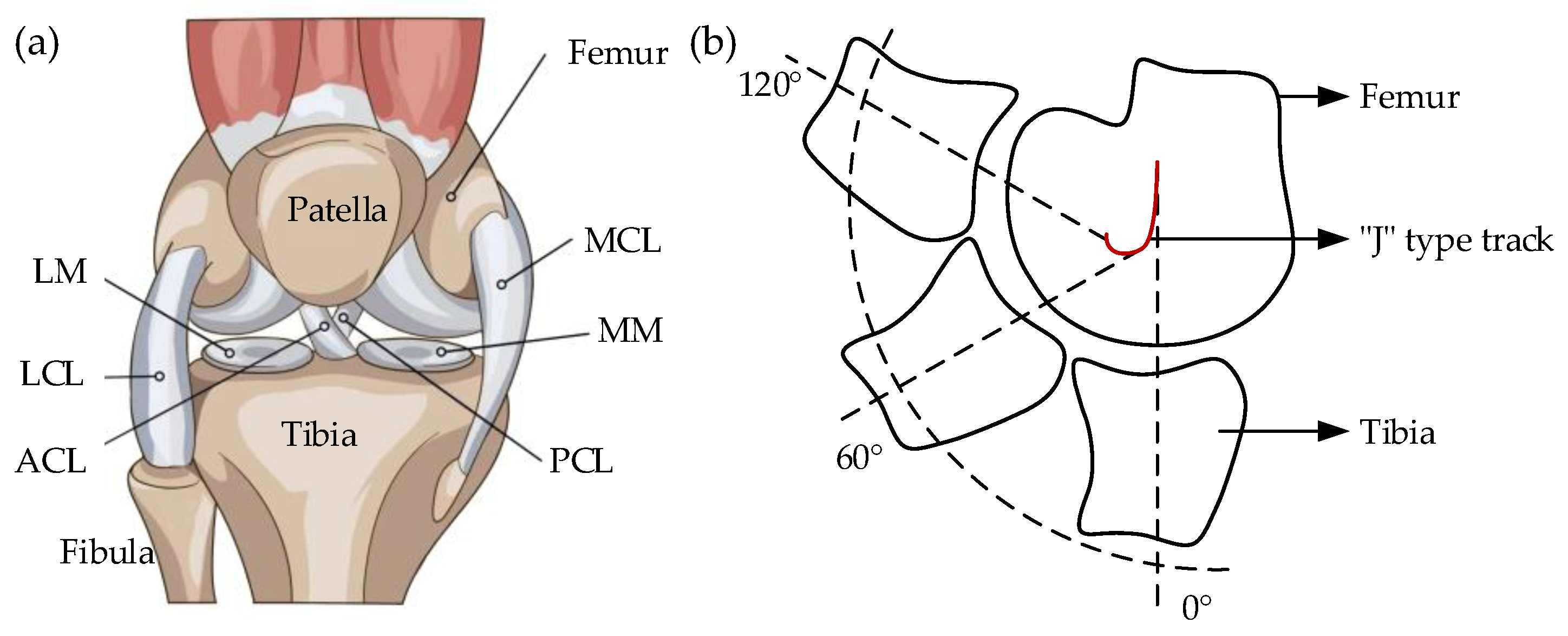
Figure 1. Composition and movement of the human knee joint. (a) An anatomical view of the human knee in the frontal plane, and (b) the ideal instantaneous center trajectory during knee joint movement in the sagittal plane [18].
Machines 11 00709 g001
Figure 2. The experimental setup and marker points. (a) The three-dimensional motion acquisition experimental setup. (b) A schematic diagram showing marker points during the motion data collection process.
Machines 11 00709 g002
Figure 3. The spatiotemporal motion of the marker points in the sagittal plane. (a) The spatiotemporal data for the marker points within a single gait cycle. (b) The macroscopic spatiotemporal data for each marker point under the fixed thigh marker point position and defined as the coordinate (0, 0) state.
Machines 11 00709 g003
Figure 4. Schematic diagram showing the feature point motion analysis.
Machines 11 00709 g004
Figure 5. Characteristic point motion of thigh fixation state.
Machines 11 00709 g005
Figure 6. Simulation model of the cross-four-bar mechanism.
Machines 11 00709 g006
Figure 7. Schematic diagram showing the optimization process.
Machines 11 00709 g007
Figure 8. Compatibility of the single degree of freedom exoskeleton motion.
Machines 11 00709 g008
Figure 9. Knee exoskeleton configuration. (a,d) use a single-hinge and a cross-four-link, respectively, with the addition of movable pairs to form (b,e). Based on this above, (c,f) additionally add ball joints.
Machines 11 00709 g009
Figure 10. Top view (left) and side view (right) of the simplified model.
Machines 11 00709 g010
Figure 11. Changes in hip and knee angles. (a,b) are comparative analysis of simulation results and theoretical calculation results for the hip and knee joints, respectively.
Machines 11 00709 g011
Figure 12. Establishing a simulation model.
Machines 11 00709 g012
Figure 13. Comparison of Simulation and Experimental Test Results.
Machines 11 00709 g013
Figure 14. Changes in radial torque at the human–machine connection. (a,c) The torque–time variation curves during a period of motion. (b,d) The corresponding box plots.
Machines 11 00709 g014
Figure 15. Changes in axial force at the human–machine connection. (a,c) The force–time curves during a period of motion. (b,d) The corresponding box plots.
Machines 11 00709 g015
Table 1. Ideal coordinate value for the instantaneous center of the knee [19].
Knee Flexion Angle/° x p / mm y p / mm Knee Flexion Angle/° x p / mm y p / mm
0007014129
1031478012130
2031879011131
30261071009132
40211181107132
50181241205133
60161271302133
Table 2. Optimization results for each parameter.
Parameter l 1 / mm l 2 / mm l 3 / mm l 4 / mm θ 1 / rad θ 4 / rad
Value34.13134.12649.62646.6670.1750.523
Table 3. Parameters of the D-H model.
L i α i a i d i θ i
1000 θ 1
20 L 1 0 θ 2
30 L 2 0 θ 3
Table 4. Regression equation coefficients for rotational inertia.
Body SegmentCoefficientMass (kg)Center of Mass (mm) I X   ( k g   m m 2 ) I Y   ( k g   m m 2 ) I Z   ( k g   m m 2 )
Neck B 0 2.954069.40027,149.4025,082.1018,641.00
B 1 0.04000.510−115.80−177.30−105.00
B 2 0.00010.0137.2211.543.82
Trunk B 0 −5.0010−66.650−234,173.20−143,387.90−51,335.70
B 1 0.1110−0.3301181.00772.601702.40
B 2 0.00501.121165.8897.5533.95
Upper arm B 0 −0.323015.150−18,962.40−18,962.40−195.30
B 1 0.03000.160165.60165.603.40
B 2 0.00010.08012.2312.230.92
Forearm B 0 −0.277012.940−8113.50−7438.30−627.90
B 1 0.01600.45042.9041.3021.40
B 2 0.00010.0545.044.640.05
Hand B 0 −0.424071.620///
B 1 0.00300.340///
B 2 0.00040.013///
Thigh B 0 −0.0930−122.520−370,537.70−366,488.906527.00
B 1 0.1520−0.310428.40554.90716.50
B 2 −0.00040.235286.21280.78−14.61
Shank B 0 −0.834023.470−30,104.40−29,916.40−1777.60
B 1 0.06100.500299.00293.0079.20
B 2 −0.00020.09520.1220.09−0.33
Foot B 0 −0.71535.130///
B 1 0.0060−0.020///
B 2 0.00070.003///
Table 5. Parameter settings for various body segments.
Body SegmentSize (mm)Mass (kg)Center of Mass (mm) I X   ( k g   m m 2 ) I Y   ( k g   m m 2 ) I Z   ( k g   m m 2 )
Neck29.4876.134131.0531,460.4032,556.6017,642.00
Trunk48.19732.1001057.19565,312.3458,110301,949.50
Upper arm33.1532.107171.1515,471.6016,171.101715.70
Forearm25.0181.103143.894176.004011.201067.10
Hand15.7150.521120.52///
Thigh44.10010.587277.23176,770.30180,532.6033,966.50
Shank51.3003.381231.9728,536.6028,220.603568.40
Foot7.2700.99539.03///
Table 6. Simulation Model Contact Parameter Settings [28].
ParameterVariableValue
Stiffness (N/mm) k 100
Force index F e 1.5
Damping (N·s/mm) D 1.0
Penetration depth (mm) P 0.0
Static friction coefficient μ s 0.3
Dynamic friction coefficient μ d 0.3
Table 7. Analysis of Moment and Axial Force at the Binding Structure.
ParameterGroup 1Group 2
SH1SH2SH3FBL1FBL2FBL3
Torque_BT
(Nm/kg)
Mean (10−4)115.4−139.6−15.1−2256.2−100.3−95.4
Median (10−4)20.667.3150.3−466.945.5−14.5
R ( m i n , m a x ) (10−2)168.1345.1297.2242.0322.1287.2
D ( Q 0.25 , Q 0.75 ) (10−3)73.9289.1308.6486.3227.8218.8
Torque_BS
(Nm/kg)
Mean (10−4)−16.716.85.0165.8101.25.4
Median (10−4)1.2−34.73.6115.330.83.0
R ( m i n , m a x ) (10−2)27.654.39.026.357.07.3
D ( Q 0.25 , Q 0.75 ) (10−3)12.341.14.037.143.23.7
Force_BT
(N/kg)
Mean (10−4)74.5116.896.0−32.8117.5105.4
Median (10−4)64.122.158.6−55.935.866.5
R ( m i n , m a x ) (10−2)12.542.620.516.726.021.3
D ( Q 0.25 , Q 0.75 ) (10−3)11.721.917.116.921.816.4
Force_BS
(N/kg)
Mean (10−4)32.39.47.5−68.910.18.5
Median (10−4)13.81.94.1−38.02.65.8
R ( m i n , m a x ) (10−2)12.73.71.212.72.81.4
D ( Q 0.25 , Q 0.75 ) (10−3)5.51.81.417.01.91.4
Bold: The minimum value of torque or force in SH and FBL schemes is highlighted in bold.
Disclaimer/Publisher’s Note: The statements, opinions and data contained in all publications are solely those of the individual author(s) and contributor(s) and not of MDPI and/or the editor(s). MDPI and/or the editor(s) disclaim responsibility for any injury to people or property resulting from any ideas, methods, instructions or products referred to in the content.