Abstract
Functional electrical stimulation (FES) has been widely used to treat spinal cord injury (SCI) patients. Many research studies employ a closed-loop FES system to monitor the stimulated muscle response and provide a precise amount of charge to the muscle. However, most closed-loop FES devices perform poorly and sometimes fail when muscle nonlinearity effects such as fatigue, time delay response, stiffness, spasticity, and subject change happen. The poor performance of the closed-loop FES device is mainly due to discrepancies in the feedback control algorithms. Most of the existing feedback control algorithms were not designed to adapt to new changes in patients with different nonlinearity effects, resulting in early muscle fatigue. Therefore, this research proposes an adaptive sliding mode (SM) feedback control algorithm that could adapt and fine-tune internal control settings in real-time according to the current subject’s nonlinear and time-varying muscle response during the rehabilitation (knee extension) exercise. The adaptive SM feedback controller consists mainly of system identification, direct torque control, and tunable feedback control settings. Employing the system identification unit in the feedback control algorithm enables real-time self-tuning and adjusting of the SM internal control settings according to the current patient’s condition. Initially, the patient’s knee trajectory response was identified by extracting meaningful information, which included time delay, rise time, overshoot, and steady-state error. The extracted information was used to fine-tune and update the internal SM control settings. Finally, the performance of the proposed adaptive SM feedback control algorithm in terms of system response time, stability, and rehabilitation time was analysed using a nonlinear knee model. The findings from the simulation results indicate that the adaptive SM feedback controller demonstrated the best control performance in accurately tracking the desired knee angle movement by having faster response times, smaller overshoots, and lower steady-state errors when compared with the conventional SM across four reference angle settings (20°, 30°, 40°, and 76°). The adaptive feedback SM controller was also observed to compensate for muscle nonlinearities, including fatigue, stiffness, spasticity, time delay, and other disturbances.
1. Introduction
Spinal cord injury (SCI) is caused by diseases or accidents that destroy the neural tissue of the spinal cord, as well as trauma that compresses, stretches, or tears this tissue. SCI is often irreversible, resulting in a partial or total loss of sensory function, paralysis, or both in areas of the body below the level of the lesion. An electrical current can be applied to excitable tissue to support or replace lost function in people with neurological disabilities. The electronic appliance that generates these electrical current pulses is a functional electrical stimulation (FES) device. The FES device causes an action potential in the neuronal axons by transmitting an electrical stimulation charge into the neural tissue. The administered stimulus charge depolarizes the neuron membrane artificially, producing an action potential that induces muscle contraction in the motor neurons [1]. The neurons are stimulated by a series of brief electrical pulses delivered via electrode pads [2]. Applying electrical currents to the motors of intact peripheral nerves makes it possible to contract paralysed or paretic muscles.
One of the essential areas in the healthcare industry is the rehabilitation of SCI patients using FES-assisted devices. The intervention of the FES-assisted device in rehabilitation exercises enables muscle movement through electrical stimulation to build voluntary strength. FES systems used to restore the loss of neurological control are also known as neuroprostheses. Examples of neuroprosthetic devices used in rehabilitation exercises are gripping, elbow extension, standing, walking, cycling, rowing, knee extension, and sitting down from a standing posture [3]. Over the last three decades, FES-assisted exercise has piqued the interest of doctors, engineers, and researchers. The development of such systems continues, with new technologies and methodologies being developed [4,5,6,7,8].
A stimulator controller is essential to any FES-assisted exercise system as it affects exercise efficiency. The FES device’s stimulation charge is administered directly to the targeted muscle to produce muscle force. It is considered a success if the stimulator controller can adapt to unpredicted muscle behaviour. However, the significant challenges faced in the design of an FES-assisted system are the nonlinearity of the musculoskeletal system and the rapid change in muscle properties due to fatigue [5,6], imprecise muscle force/torque control [6], spasticity [3,9], time-varying delay [10,11,12], and day-to-day variation [5,6,13,14,15]. As a result, more research is needed to design a control technique or algorithm that provides satisfactory tracking performance; is robust against time-varying properties of muscle dynamics, day-to-day variations, subject-to-subject variations, muscle fatigue, and external disturbances; and is simple to apply across experiment sessions [3,5,12,16,17]. Therefore, to design a robust controller for an FES-assisted device, all of the factors mentioned above must be fully considered for further investigation.
Most FES devices on the market use an open-loop stimulation strategy for neuromuscular applications to achieve the desired movement. Open-loop control systems, which need continual trial-and-error input from the operator, ultimately result in an early onset of muscle fatigue [4,18]. This is because the conventional stimulation technique of the current FES device, which typically employs a single open-loop stimulation channel, delivers a fixed stimulation pattern on the same motor unit synchronously, which results in the motor unit being overworked [3,5]. Furthermore, because of existing parameter variations (e.g., muscle fatigue), inherent time variation, time delay, and strong nonlinearities in the neuromuscular-skeletal system, the open-loop control FES performance was found to be unsatisfactory for accurate movement control [3,19]. Therefore, a feedback controller is needed to precisely control the generated movement due to the underlying neuromusculoskeletal system’s highly nonlinear and time-varying nature. A closed-loop FES system, which uses a feedback controller to monitor the stimulated muscle response and deliver the appropriate amount of charge to the muscle, has been proposed by numerous researchers as a solution to the open-loop control system problem in FES [4,5,6,17,20]. Several types of feedback controllers have been commonly used in the closed-loop FES system, which include proportional−integral−derivative (PID) [3,21,22], fuzzy logic (FL) [4,5,6,23], neuro-fuzzy [24], sliding mode (SM) [3,5,9,19], gain scheduling (GS) [3,25], and artificial neural network (ANN) [26,27].
Among the existing feedback control algorithms, the PID controller is mainly used by researchers in FES applications due to its simplicity, ease of implementation and tuning, and high degree of familiarity. However, the comparative study of closed-loop controllers conducted by a few researchers has indicated that the performance of PID controllers was degraded when muscle nonlinearity effects were included in the simulation [3,23]. The presented results demonstrate that the classical PID controller alone was not a suitable technique for practical FES applications due to its inferior performance in successfully regulating electrically stimulated muscle contractions when nonlinearity effects were considered [3,23]. An intelligent controller such as fuzzy logic is very popular, has a better capability of adapting to the dynamic characteristics of the muscles, and has long been recognised for its ability to manage a complex nonlinear system without creating a complex mathematical system model [6,23]. The fuzzy logic (FL) controller could also be tuned in real time, has less chattering, and performs better than the PID controller [28,29]. However, the FL controller has lower control bandwidth and convergence limitations, which result in slow joint movements in FES [30,31]. Furthermore, the FL controller is incapable of generalizing, or it only responds to what is written in its rule base and is not robust concerning topological changes in the system. Such changes in the system would necessitate changes in the FL controller rule base and limitations in updating the membership function and consequent parameters to obtain reasonable results [32,33]. Artificial neural networks (ANNs) are an attractive control technique for FES applications because they mimic how the brain is assumed to regulate muscle contractions. However, these techniques typically do not guarantee stability, which should be considered a mandatory control requirement for a system that interfaces with human users, such as FES applications. Another disadvantage of neural networks is that they are too slow for online adaptation, which requires lots of data in which the expected nonlinear conditions must be present during data training to make them work effectively, and thus need to be trained offline [19]. In the case of parameter variation, when FES is applied to different subjects, neural networks often need to be retrained, which is a time-consuming procedure [19]. Furthermore, when the network is overtrained, it suffers from overfitting, which results in poor generalisation when unseen data patterns are introduced to the system or when the system complexity is greater than the training data [34].
A modern controller such as sliding mode (SM) is also known for its robustness in dealing with uncertainties, nonlinearities, unmodeled dynamics, quickly varying parameters, and external disturbances [3,5,9]. Additionally, the SM controller was found to provide fast tuning and exhibit the best sinusoidal tracking performance [3]. However, the disadvantages of this SM controller are that it suffers from chattering [3,9,35] and requires a mathematical model to design the sliding surface [19,21]. The performance of this controller might be improved by using a more accurate model of the stimulated muscle response that includes nonlinearities or by using a different method to overcome the chattering problem. The gain scheduling (GS) controller works acceptably well for FES systems, but choosing a suitable scheduling variable that captures the system’s nonlinear behaviour is challenging. Moreover, the GS controller involves a lengthy tuning process because it uses multiple local controllers. This tuning process may have to be repeated daily to accommodate variations in the response of the stimulated muscles [3].
Although numerous types of feedback control algorithms have been used in the FES system for knee extension, Cheryl et al. (2012), Jazernik et al. (2004), and Montazeri et al. (2021) concluded that none of these feedback controllers was ready for real-world FES applications yet [3,5,19]. While it is expected that closed-loop control will improve the control performance, the actual performance of closed-loop controllers is insufficient for real-world applications because most feedback controllers exhibit a significantly degraded performance when real-world nonlinear effects of muscle, such as time-varying delay response, fatigue, stiffness, and spasticity, are considered [2,3,5,17,19]. This is because most existing feedback control algorithms were not designed with a system identification feature and an automatic tuning mechanism that can detect and quickly adapt to new system changes according to the subject’s muscle response and other nonlinear disturbances such as muscle fatigue, time delay, stiffness, and spasticity [13,14,15,17,20]. The feedback controllers were tuned only during the simulation design stage, where fatigue and other nonlinear disturbances were either not included or represented by a single predicted value to represent the nonlinear response of the muscle model [14,17]. However, the nonlinear effects of actual human muscles vary with time, and different subjects have different nonlinear muscle responses. Therefore, any new changes or disturbances that occur when a closed-loop FES system is in operation, such as different human subjects, nonlinear time-varying muscle response, and other disturbances (fatigue, stiffness, and spasticity), will cause changes in the FES system. This resulted in the internal control settings of the feedback control algorithm, which were obtained during the design phase, being no longer accurate and suitable for the real-world closed-loop FES controller [17]. The nonlinear muscle response causes the overall system to change, resulting in the feedback controller having an under performance and providing an inaccurate amount of stimulus charge to the patient [3,5,19]. The inaccurate amount of charge might lead to overstimulation, early muscle fatigue, and, consequently, muscle damage [36].
The nonlinear response of human muscle and other disturbance factors such as muscle fatigue, stiffness, and spasticity during FES-assisted activities has led to a time-varying delay response in the FES system. The large time delay in the real-world FES application will result in a poor performance of the closed-loop FES controller due to oscillation and stability issues. The time-varying delay becomes more obvious as the fatigue increases [13,37]. Most existing feedback controllers have no specific method to handle this large time-varying delay response.
Therefore, besides providing an accurate nonlinear knee model during the simulation stage, the design of feedback control algorithms in a closed-loop FES system must be significantly improved before they can be implemented in real-world applications [3,5,16,17]. Real-world FES devices must be able to accurately adjust the electrical stimulation pulse in real time to account for nonlinear muscle effects, such as time-varying delay responses, fatigue, spasticity, and retraining effects [3]. The conventional controller can only perform control loops to maintain the control variables at a dedicated set point. However, once the process starts to operate beyond such variables, the changes in functionality can be carried out by employing adaptive control [38]. To overcome the limitations of existing feedback control algorithms, much of the current research uses adaptive control methods in the FES closed-loop system [9,15,22,35,39,40,41,42]. Adaptive control is the control method a controller uses to adapt to a controlled system with parameters that vary or are initially uncertain [43].
The adaptive controller can be divided into a few categories, which are gain scheduling [3,25], self-tuning regulators [44,45], iterative learning controllers [46,47], feedforward controllers [48,49], model reference adaptive controllers (MRAC), and model identification adaptive controllers (MIAC) [50,51]. These last two adaptive controllers (MRAC and MIAC) utilise several feedback control units, such as PID, FL, NN, SM, and others, as part of their systems. The MIAC controller has a system identification to identify the status of the controlled system and to determine the relevant control laws and gain so that adjustments can be made to the feedback control unit settings [39,52]. Meanwhile, the MRAC type compares the observer and actual system outputs to adjust the system’s state variable under control. An observer can also be used in the MIAC type of adaptive controller, becoming a hybrid of the MIAC and MRAC adaptive controllers [50,51,52].
Several adaptive feedback control algorithms have recently been published to overcome the limitations of existing closed-loop FES. Kobravi and Erfanian (2012) used fuzzy logic as part of the adaptive system and the second-order SM controller in a complete adaptive system dealing with unknown and dynamic nonlinearities to control standing [35]. Fuzzy logic was used as a state variable representation. Sharma et al. (2017) employed integrator backstepping with a neural network used to estimate the state variables and the second-order SM controller to control knee extension in the presence of unknown dynamic nonlinearities and specific nonlinearities of fatigue and spasticity [53]. Cousin et al. (2022) used an SM with a feedforward neural network as an adaptive admittance controller for cadence rehabilitation to deal with unknown and dynamic nonlinearities [42]. Ajoudani and Erfanian (2009) used a neuro-sliding mode adaptive controller for controlling paralysed limbs in knee extension. Two neural networks were used to represent state variables to eliminate chattering [9]. Cousin (2020) employed two neural networks for adaptive admittance control of hybrid exoskeletons for the knee and ankle joints to deal with disturbances and unknown nonlinearities. The Lyapunov method was also used for stability [15]. Naoual et al. (2014) used an adaptive Takagi-Sugeno fuzzy SM for two-link robot exoskeletons against nonlinearities of dynamics, uncertainties, and disturbances of the exoskeleton’s motors [41]. Riani et al. (2018) used an integral terminal SM to eliminate singularities and dynamic uncertainties, resulting in less output chattering due to changes in person [40]. Wang et al. (2013) used an adaptive controller made of PD and a neural network to compensate for unstructured uncertainties [54]. JoAnne Riess (2000) employed a neural network and PD in combination as an adaptive feedforward, whereby the neural network was used to generate stimulation patterns to tackle the dynamic uncertainties of a nonlinear system of the shank [55]. Asadi and Erfanian (2012) used two adaptive neuro-fuzzy sliding modes to control rat ankles for flexor and extensor muscles in dynamic uncertainties [24]. Belkadi et al. (2017) reported that the adaptive PID controller with the modified PSO algorithm provided satisfactory results in tracking the desired trajectories in position and velocity [21]. Bkekri et al. (2019) reported that the robust adaptive SM controller for human-driven knee joint orthoses had a good tracking performance [56]. Li et al. (2020) used an adaptive controller to incorporate human and robot capabilities for knee-climbing trajectories [57]. Montazeri et al. (2021) successfully designed and simulated the fuzzy adaptive sliding mode controller to track the reference trajectories in the presence of time-varying system parameters, external disturbances, muscle fatigue, and unmodeled dynamics [5].
Although several authors have claimed success for the proposed adaptive feedback controller and control techniques or algorithms, no detailed analyses have been provided on how the proposed controller could handle specific nonlinearities such as fatigue, stiffness, spasticity, and time delay. Additionally, none of the published works has proven in detail that the proposed adaptive feedback control algorithms could still maintain their performance and compensate for each specific nonlinearity effect, which includes stiffness, spasticity, external disturbance, and time delay. To the best of the authors’ knowledge, no published work has demonstrated that the proposed feedback controller can optimize, maximize, or extend the duration of rehabilitation exercise and compensate for fatigue by adaptively changing the reference angle during the exercise. Therefore, many areas for improvement can still be studied and investigated for lower limb rehabilitation, such as knee extension involving FES. For instance, the adaptive type of MIAC controller has not been studied or found in the literature.
This paper proposes an adaptive SM feedback control algorithm for a closed-loop FES system that could monitor the progress of knee extension movement and ensure the closed-loop FES delivers an appropriate amount of stimulus charge according to the status of the patient under treatment. The adaptive SM feedback control algorithm was designed to automatically adjust the relevant internal control settings for self-tuning in real time to fit the condition of patients undergoing rehab treatment. The adaptive self-tuning of the feedback control algorithm ensures the closed-loop FES device delivers a precise amount of charge, indirectly preventing early muscle fatigue and consequently prolonging the rehabilitation exercise. The adaptive SM feedback controller consists mainly of a main control unit with a system identification feature and a tuneable SM feedback control unit. Initially, three conventional feedback control units (FCUs)—namely, PID, FL, and SM—were developed and tuned using particle swarm optimization (PSO). Then, the performances of the three FCUs regarding rise time, overshoot, steady-state error, and oscillation were evaluated. The SM feedback control unit was chosen for the adaptive feedback controller implementation in this work because it performed the best out of the three FCUs. Two types of knee extensions, namely physical-based and numerical models, were designed and developed with muscle nonlinearities such as fatigue, time delay, stiffness, and spasticity. The feedback controllers and the knee extension model were designed and developed in the MATLAB Simulink (Mathworks, Portola Valley, CA, USA) environment. Finally, the performance of the adaptive SM feedback controller in terms of system response time, stability, steady-state error, and rehabilitation time was analysed using the developed nonlinear knee extension model.
This paper is organised as follows: Section 2 presents the design methodology for the adaptive feedback control algorithm’s implementation. The explanation starts with a system overview of the closed-loop FES with an adaptive feedback controller for the knee extension application. After that, the implementation of the nonlinear knee extension models, the design of FCUs (PID, FL, and SM), and an adaptive SM feedback controller are elucidated. Each design phase is explained in detail, starting from modelling the nonlinear knee model using a physical-based model and numerical computation method, designing FCUs (PID, FL, and SM), tuning the designed FCUs using PSO, designing the adaptive SM feedback control algorithm, extracting the essential features from the knee response, and establishing the control laws and look-up table (LUT) of data after the optimization process. Section 3 discusses the performance of the three FCUs (PID, FL, and SM) from the obtained simulation results, and the performance of the adaptive SM feedback controller. In this section, the performance of the designed adaptive SM feedback controller is discussed and compared with the conventional SM feedback controller and from other research work. Finally, Section 4 presents the conclusion of the research work.
2. Materials and Methods
This section discusses the design methodology of the nonlinear knee extension model, the design and fine-tuning process of conventional FCUs (PID, FL, and SM) using PSO, and the implementation of an adaptive SM feedback controller. In this research, three main design phases were executed to implement an adaptive SM feedback controller for a nonlinear knee extension model. All design phases were implemented and tested using the MATLAB Simulink environment. The design process started with modelling the nonlinear knee extension for a closed-loop FES knee extension application. For performance comparison purposes, three FCUs, including SM, PID, and FL, were initially developed and fine-tuned at a reference angle of 40° using PSO. During the tuning phase, the key performance indicators of these FCUs in terms of rise time, overshoot, steady-state error, and oscillation were evaluated using a digital signal processing method to obtain the optimised gain settings (for SM and PID) and membership function (for FL). After the optimised gain and membership function settings were obtained, the three FCUs were tested with the nonlinear knee model. During the testing phase, the FCU that demonstrated the smallest value for rise time, settling time, overshoot, and steady-state error was selected for the adaptive feedback controller implementation. Additionally, the FCU that performed well at four reference angles (20°, 30°, 40°, and 76°), and that was robust against disturbances and nonlinearities was also taken into consideration as the best controller. Finally, among the three FCUs (PID, FL, and SM), the one with the best performance was chosen for the adaptive feedback controller implementation. The SM FCU, which exhibited the best performance, was fine-tuned once more to achieve optimal gains at a few ranges of reference angles (20°, 30°, 40°, and 76°) for adaptive controller implementation. Once the fine-tuning process of the SM feedback controller was completed, the optimised gains at different reference angle settings were stored in a look-up table (LUT) for reference. The adaptive SM feedback controller was then tested with the nonlinear knee extension model for performance evaluation. The following subsections provide detailed explanations of the nonlinear knee extension model development, the development of three FCUs (SM, PID, and FL), the tuning and performance evaluation of three FCUs (SM, PID, and FL) using PSO, and finally the design and testing of an adaptive SM feedback controller.
2.1. System Overview of Adaptive Feedback Controller
The proposed adaptive feedback controller was designed to control and generate an appropriate FES signal to maintain knee extension at a specific angle over long periods of rehabilitation exercise, to maintain control performance at different reference angles, to compensate for nonlinearity effects, and to be robust against external (sensors, FES device, power supply noise), and internal (model mismatch, muscle nonlinearities, and unknown dynamics) disturbances. Figure 1 depicts the basic system overview of an adaptive feedback controller with a nonlinear knee model.
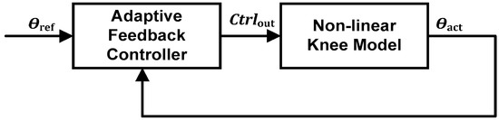
Figure 1.
System overview of an adaptive feedback controller.
The position error obtained from the comparison between the reference angle ( and the actual angle ( is calculated internally in the adaptive feedback controller to determine the appropriate control output signal (Ctrlout) or stimulus pulse that needs to be provided to the knee model.
2.2. Knee Movements and Maximum Muscle Torque for Knee Extension Model
The knee angle depicted in Figure 2 indicates the estimated knee movement of an SCI patient and its equivalent model using the closed-loop FES device.
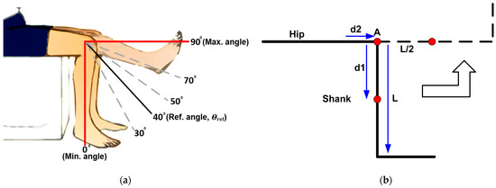
Figure 2.
Knee extension body mechanics: (a) knee extension; (b) knee extension equivalent model.
An illustration of knee movements from a resting position (0°) to a fully extended position (90°) is shown in Figure 2a. The knee angle is 0° in rest mode and remains in that position until the FES device provides a stimulus charge to the quadriceps muscles. The muscle contracts due to the administered stimulation charge, resulting in a knee extension movement. The angle (θact) generated by the limb’s movement is used as a feedback input by the adaptive feedback controller to calculate the amount of charge that must be adjusted throughout the stimulation operation. An example of a knee extension movement targeted to achieve a 40° reference knee angle (θref) is shown in Figure 2. Two types of input data can be derived from θref and θact. The first input datum is error (e), which is the difference between θref and θact. The second input datum is the change in error (de), which is the difference between the current and previous errors. The error (e) and error change (de) can be specified using Equations (1) and (2):
The adaptive feedback controller uses these input data ( and ) to calculate the amount of charge (pulse width duration) required to meet the targeted reference angle (θref). While negative denotes overstimulation of the charge, positive indicates that the applied charge is still insufficient. As a result, the feedback controller adjusts the stimulus pulse width (ΔT) appropriately (increasing or decreasing) until the desired target angle is reached [4]. Details of input data ( and ) processed by the feedback controller are explained in the following sections.
The body mechanics of the knee movement are then illustrated in Figure 2b for muscle torque calculation. The maximum muscle torque of a knee extension model is calculated by considering the human body weight of 117 kg with a lower leg weight of about 7 kg. Muscle torque is calculated by considering the body mechanics of knee movement. For knee extension modelling, a weight of 7 kg for the lower leg is used, and the centre of mass is 0.16 m of the total shank length (L), as shown in Figure 2b. The distance from the muscle pivot to the end of the muscle tendon (d2) is averaged at 1/5 of the shank length (L), which is 0.064 (0.32/5) metres. Consider the sum of moments at the knee pivot (A) for muscle torque calculation, as shown in Figure 2b. The muscle torque output calculations are shown in Equations (3)–(11), as listed below:
where,
| TA | : | Summation of torque at point A |
| m | : | Shank weight (7 kg) |
| g | : | Gravity (9.81 m/s2) |
| d1 | : | Half of the shank length |
| d2 | : | Muscle pivot |
| F | : | Force |
| L | : | Shank length |
| Tq | : | Muscle torque = F × d2 |
In this work, the muscle torque needed to lift a 7 kg weight with a lower leg from rest (0°) to full extension (90°) was calculated to be 10.99 Nm. Thus, the maximum muscle torque of 10.99 Nm was used as a reference for the maximum knee extension of 90°.
2.3. Nonlinear Knee Extension Model Development
Figure 3 depicts the internal block diagram of the nonlinear knee extension model. The developed nonlinear knee extension model consists mainly of the first-order muscle model (torque), the basic second-order Veltink’s knee extension model, and the nonlinear muscle models, which include time delay, fatigue, stiffness, and spasticity. The basic second-order knee extension model was designed following the Veltink et al. (1992) model [58], and the nonlinear muscle model parameters (time delay, fatigue, stiffness, and spasticity) were developed following the Lynch and Popovic (2012) and Ferrarin and Pedotti (2000) methods [3,59]. One new parameter for the nonlinear muscle model was time delay.
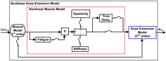
Figure 3.
The internal architecture of the nonlinear knee extension model.
The overall nonlinear knee extension model was first designed and developed using a physical-based model and later converted into a numerical model using Taylor series computation. This is because the conventional physical-based model may take some time to converge during tuning when running with the optimization tool. To increase the convergence’s speed while maintaining the system’s accuracy, the knee model is best represented in discrete form or numerical computation [60]. Therefore, the conversion of the physical-based model into a numerical computation model was done to increase convergence speed during the fine-tuning process using PSO.
When applied to the first-order muscle model, the feedback controller’s output (Ctrlout), in terms of stimulus pulse width, generates force, which is later converted into muscle torque. The muscle torque causes the knee extension movement after the second-order knee model. The muscle model’s nonlinear components, including fatigue, spasticity, time delay, and stiffness, were also modelled and incorporated into the system for feedback controller development, testing, and analysis purposes. Detailed explanations for each internal block are provided in the following subsections.
2.3.1. Second-Order Knee Extension Model
The second-order knee extension movement was modelled based on the mechanics of the human body using Veltink et al.’s (1992) control model [58]. As depicted in Figure 2, muscle force is required to lift the lower leg with no other load for the knee extension movement. The muscle force to lift the lower leg is converted into muscle torque by multiplying the muscle force by the acted muscle tendon distance. The Veltink et al. (1992) knee extension control model represents the limb parts, as shown in Figure 2a. The movement is described by a second-order equation that relates the torque and angle, as defined in Equation (12):
The physical-based model can be formed as in Equation (13):
where,
| M | : | Joint torque |
| θ | : | Joint angle |
| : | Joint angle velocity | |
| : | Joint angle acceleration | |
| θnom | : | The angle at which the steady-state torque equals zero |
| I | : | Inertia |
| B | : | Damping |
| C | : | Compliance with the load = |
| m | : | Shank Weight (7 kg) |
| l | : | Length to the centre of the shank |
| g | : | Gravity (9.81 m/s2) |
The Veltink et al. (1992) second-order knee extension control model is much simpler to implement and more linear, as it does not contain any nonlinear functions of sin or cosine in its mathematical model [58]. The mathematical model of the Ferrarin and Pedotti (2000) knee extension model has a sine function, which makes the system nonlinear [59]. The muscle models designed by Reiner et al. (1996 and 2002) focused on the muscle without the biomechanics of the knee extension model [7,8].
2.3.2. Nonlinear Muscle Model
The muscle nonlinearity effects, which include fatigue, time delay, stiffness, and spasticity, are incorporated into the knee model for accurate knee model representation. In this work, the muscle nonlinearities’ equations are combined to form a physical-based model and later converted into numerical computation. The muscle can also be modelled using a non-mathematical approach, such as fuzzy logic, genetic algorithm, and ANFIS, as reported by Ibrahim et al. (2011) [61] and Salleh et al. (2013) [62]. Detailed muscle nonlinearities, which include fatigue, time delay, stiffness, and spasticity, are explained in the following subsections.
- Fatigue
The fatigue effect causes muscle torque to decrease over time, and when the overstimulation effect persists, the fatigue effect increases [53]. Fatigue is implemented as a multiplier that modifies the electrically stimulated quadricep muscles’ torque [3]. The value of the fatigue waveform ( ranges between 0 and 1 in the time domain, with 1 corresponding to no fatigue and 0 corresponding to no measurable response to stimulation [3]. The higher the fatigue effect, the faster the torque input decreases. Equations (14) and (15) represent the fatigue effect in the time domain for mild and severe fatigue [63].
- 2.
- Stiffness
The muscle stiffness was designed based on Lynch and Popovic (2012) [3] and Ferrarin and Pedoti’s (2000) [59] models. The stiffness effect is according to Equation (16).
Stiffness causes a reduction in muscle torque when the movement starts from a standstill and disappears when the knee trajectory angle reaches a certain degree of resting elastic knee angle () [3].
- 3.
- Time Delay
The muscle time delay nonlinearity is challenging as it can cause the system to become uncontrollably unstable. The transfer function first order plus time delay () is given by Equation (17). The exponential term represents a time delay [64].
where,
| τs | : | Time constant |
| K | : | System gain |
| θS | : | Delay angle (in transfer function format) |
The Pade approximation was used to represent the time delay, allowing the root locus, bode plot, linear quadratic regulator (LQR), and H infinity controllers to work. In this work, the time-delay effects were developed using MATLAB Simulink transportation delay in the range of 10 ms (minimum) to 260 ms (maximum) [11,12,30,65].
- 4.
- Spasticity
The spastic hamstring torque is expressed as in Equation (18) [3].
where is the hamstring tension resulting from the spasm. We assumed that = 5 cm was the distance between the centre of rotation of the knee and the insertion point of the biceps femoris on the fibula. The angle between the longitudinal axis of the hamstrings and the axis of the shank can be expressed as in Equations (19) and (20).
The hamstring tension was determined by
where Td = 40 ms was the delay between the stretch and the onset of the resulting contraction, and was the maximum spastic torque elicited at the maximum knee angular velocity [3].
2.4. Design and Development of Feedback Control Units
The three FCUs, namely PID, FL, and SM, were first developed using MATLAB Simulink. Details for each controller are explained in the following subsections.
2.4.1. Design and Implementation of PID Control Unit
The PID controller was developed based on the mathematical equations represented in the Laplace transform, shown in Equations (21)–(25). From the equations, represents the PID controller’s output signal (Ctrlout) or stimulus pulse that needs to be provided to the knee model.
where,
| Kp | : | Proportional controller gain |
| Ki | : | Integral controller gain |
| Kd | : | Derivative controller gain |
| Td | : | Derivative time |
| Ti | : | Integration time |
| u(t) | : | Controller output in the time domain |
| e(t) | : | Error in the time domain |
| u(s) | : | Controller output in s domain |
| e(s) | : | Error in s domain |
The PID controller’s final gain settings ( were determined during PSO tuning optimization. The PID equations were then transformed into an algorithm that works on discrete controllers.
2.4.2. Design and Implementation of FL Control Unit
As indicated in Figure 2, the angle (θact) generated from the limb’s movement serves as the feedback input to the FL control unit to determine the required amount of charge during the stimulation operation. The error () and change of error () shown in Equations (1) and (2) are initially calculated for the FL control unit’s input data. The FL control unit processes these input data ( and ) to determine the amount of charge (pulse width duration) required to meet θref.
Trapezoidal and triangular shapes are used to define the membership function (MF) and degree of MF. The MFs for errors () and changes in errors (), which include the negative big (NB), negative small (NS), zero (ZE), positive small (PS), and positive big (PB), are shown in Figure 4. As depicted in Figure 4 and described in Table 1, the limits of the triangle MFs for error (e) and change in error (de) are equally divided.
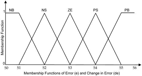
Figure 4.
Membership function (MF) of error (e) and change in error (de). The input MFs are negative big (NB), negative small (NS), zero (ZE), positive small (PS), and positive big (PB).

Table 1.
Membership function (MF) of error (e) and change of error (de). The input MFs are negative big (NB), negative small (NS), zero (ZE), positive small (PS), and positive big (PB).
The Takagi–Sugeno singleton method was employed to represent the output of the MF due to its simplicity and reduced computational complexity [4]. In this Takagi–Sugeno model, the singleton MFs of fuzzy output are represented as values of 1 at a single location and 0 at all other locations. Figure 5 depicts the singleton MF of the fuzzy output at a reference angle of 40°. As listed in Table 2, the 25 rules (min 1–min 25) are developed because the FL control unit has two inputs (error () and change in error ()) and five MFs (NB, NS, ZE, PS, and PB) for each input. Any combination of two linguistic variables triggers at least one rule. The 25 fuzzy singleton outputs are also referred to as c1–c25.

Figure 5.
MF of fuzzy output (reference angle = 40°). The singleton output MFs are zero (ZE), small (SM), medium (ME), big (BG), and very big (VB).
Table 2.
Fuzzy rule-based table mapping for two inputs, error (e) and change in error (de), and singleton outputs. The input MFs are negative big (NB), negative small (NS), zero (ZE), positive small (PS), and positive big (PB). The singleton output MFs are zero (ZE), small (SM), medium (ME), big (BG), and very big (VB).
Examples of fuzzy rules in IF−THEN statements for min 1–min 5 using the Takagi-Sugeno method are shown in Equations (26)–(30). These equations are generated based on the set of rules from Table 2. Similar IF−THEN statements are also applicable for min 6–min 25.
The MF output grades of each rule are accumulated into a single value to represent the final fuzzy output signal. The defuzzy output was computed using the centre of gravity (COG) approach. The advantage of this COG approach is that it can lower computational complexity and generate quick results [4]. This COG technique was implemented by multiplying the final accumulated fuzzy output from the MF output grades by its associated singleton value, then dividing this multiplied value with the final accumulated fuzzy outputs from the MF output grades, as shown in Equation (31). The defuzzy output (crisp output) represents the output signal (Ctrlout) or stimulus pulse that the FL control unit must deliver to the knee model.
2.4.3. Design and Implementation of SM Control Unit
The sliding mode (SM) control, which is one of the variable structure control (VSC) approaches, is usually used in a system for excellent disturbance rejection and set point tracking [5,66]. VSC has nonlinear feedback, which is discontinuous. SM control is nonlinear because the input switches rapidly between two or more control limits. The system’s structure can be changed or switched as it crosses each discontinuity surface, using this control as the feedback. When the trajectory moves on the sliding surface, the equivalent control operates internally and controls the system. Two types of SM controls were developed: conventional SM and second-order unchattered sliding mode (USM). The mathematical equations for the conventional SM and USM are shown in Method 1 and Method 2 below:
- Method 1: Conventional SM Control Unit
The simplest form of SM mathematical equations is listed in Equations (32)–(35) in their canonical form. The sliding surface is defined as in Equations (36) and (37); the final implementation and controller output are as in Equation (38) [3,5,9]. The gain setting for λ can be determined using trial and error, or PSO.
u represents sliding input, y represents knee angle, represents the state variable, is the state variable representing knee angle acceleration, and defines the state variable representing knee angle velocity.
Define sliding surface (s) as in Equation (36)
Define the equivalent sliding surface as in Equation (37), where is rate of error, is the gain constant, and is the error.
The derivative of Equation (37) is shown in Equation (38).
Using control law [67], u = , the controller is designed as in Equation (39)
The term is nullified by the first order, and will always go to zero in finite time. In this work, the SM controller’s final gain setting for from Equation (39) was set equal to the maximum muscle torque (), and the final gain setting for λ from Equation (37) is 0.5, which was determined during PSO tuning optimization.
- 2.
- Method 2: Unchattered SM (USM) Second order
The second-order SM is one of the best sliding mode control algorithms, significantly reducing the chattering effect [56,68]. It has good resistance against external force disturbances during knee movement and provides good tracking of the desired trajectory set by the therapist or the subject [56]. The system can be converted into canonical form, as shown in Equation (40). Feeding in state variables and parameters results in Equations (40) and (41).
where,
| I | : | Inertia () |
| B | : | Damping () |
| D | : | State variable constant (D = ) |
| M | : | Joint torque (10.99 Nm) |
| m | : | Shank weight (7 kg) |
| l | : | Length to the centre of the shank (0.16) |
| g | : | Gravity (9.81 m/s2) |
The conversion of a state-space model to a transfer function model was done using the MATLAB Simulink function (ss2tf) [69].
The sliding mode controller must be transformed into a state-space controllable form. Thus, the linear differential in Equation (12) can be written in transfer function in the time domain, as shown in Equation (43). Equations (44)–(47) are the state space in canonical form.
where
| : | knee angle | |
| : | knee velocity | |
| : | State variable | |
| : | State variable |
The state space model in the controllable canonical form [69] is shown in Equation (48).
As shown in Equation (48), the state space model has been tested using the quadratic local Lyapunov function for stability evaluation [70]. The obtained values of the P11 matrix (1.954) and determinant (0.053) are greater than 0. Therefore, the system is considered stable.
Then, the sliding surface is determined as shown in Equation (49)
e denotes tracking error and λ must be greater than zero (0). The tracking error and its derivatives can be expressed by Equations (50)–(52)
where denotes the desired position (reference angle ) and θ denotes the actual position (actual angle ). The Lyapunov function is defined by Equation (53).
To ensure stability, the derivative of the Lyapunov function must satisfy V < 0, as shown in Equation (54)
The derivation of the sliding mode function is shown in Equations (55)–(57).
Thus, the derivation of the Lyapunov function is shown in Equation (58) [66].
Substituting Equation (59) into (58), Equation (60) is obtained.
where
The controller is designed, as in Equation (60), to meet the condition of , as stated in Equation (54).
2.5. Tuning and Testing Feedback Control Units
The developed FCUs (SM, PID, and FL) were first tuned using PSO to obtain the best performance for four reference angles: 20°, 30°, 40°, and 76°. Figure 6 illustrates the tuning of three FCUs (SM, PID, and FL) using PSO with the assistance of system identification and performance evaluator units. For the FCUs’ tuning, the previously developed knee extension model using a physical-based method was first transformed into a numerical computation model using Taylor series computation for fast convergence [70].
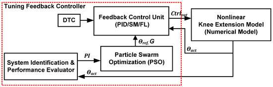
Figure 6.
Tuning feedback control units (FCUs) using PSO, system identification, and the knee extension model.
The system identification was used to extract essential features from the acquired knee trajectory output response (, which include rise time, steady-state error, and overshoot, for system performance evaluation during the tuning phase in order to find the best gain settings for the FCUs (SM, PID, and FL).
The PSO used 50 particles, representing the possible gains for each FCU at a reference angle of 40°. Details of the parameter settings’ range used for each FCU are listed in Table 3. This work used a reference angle of 40° to represent the medium knee angle reference during the rehabilitation exercise. Each particle was tested for 100 iterations. Therefore, for 50 particles, 5000 steps of iterations are required for each FCU. The performance of the designed FCUs (SM, PID, and FL) was evaluated in terms of their time response, overshoot, steady-state error, and oscillation. Each parameter has a performance indicator (PI) setting of 0% as the lowest mark and 25% as the highest mark. The grading performance for each parameter setting ranging from 0 to 25% is listed in Table 4. For example, the rise time is graded 0% for a duration above 5 s and 25% for a duration less than 3.3 s. Between 3.3 s and 5 s, the rise time is graded accordingly to determine the percentage mark. Similarly, for the other parameters (overshoot, steady-state error, and oscillation), specific value settings are used to grade the performance between 0% and 25%. Therefore, the combination of four parameters (rise time, overshoot, steady-state error, and oscillation) accumulates into one single PI that ranges from 0 to 100%. The highest PI represents the best performance for the tested FCU. The optimised gain (G) or MF was saved in a look-up table (LUT), and adaptive control laws were formulated for the FCU references.
Table 3.
The range of gain and membership function settings for each feedback control unit (FCU).
Table 4.
The minimum and maximum ratings for each parameter.
After the tuning process, the FCUs (SM, PID, and FL) were tested again on the four reference angles (20°, 30°, 40°, and 76°) using the nonlinear knee extension model. The knee muscle model nonlinearities, which include stiffness, fatigue, spasticity, and time delay, were included in the FCUs’ performance evaluation. The FCU incorporated a direct torque control technique (DTC) when a higher time delay (260 ms) was detected. The FCU that manifested the best performance (smallest values of rise time, overshoot, steady-state error, and oscillation) was chosen for the final implementation of the adaptive feedback controller design. The SM exhibited the best performance among the three FCUs in this work. Details of the performance analysis are provided in the Results and Discussion sections.
2.6. Adaptive Sliding Mode Feedback Controller
Figure 7 depicts the adaptive SM feedback controller’s internal architecture, consisting of a main control unit with a system identification feature, tuneable SM and USM feedback control units, a DTC, and a LUT.
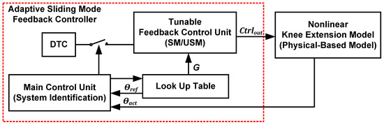
Figure 7.
The internal architecture of the adaptive SM feedback controller.
The function of the main control unit is to monitor and supervise the overall operation of the adaptive SM feedback controller. The function of the system identification feature incorporated in the main control unit is to extract essential features such as rise time, time delay, steady-state error, and overshoot from the acquired knee trajectory output response to identify the patient’s knee muscle status during the testing phase. The two types of employed FCUs, namely SM and USM, are activated according to the patient’s condition. DTC is incorporated into the adaptive controller and is activated when a larger system time delay (260 ms) is detected. LUT is used to store the optimised gain (G) and reference angle (
The adaptive SM feedback control algorithm has two primary operations, namely open-loop and closed-loop stimulations. The adaptive SM feedback controller’s operation begins with an open-loop stimulation. The main control unit initiates open-loop stimulation by sending a preset pulse width value (corresponding to a medium reference angle of 45°) to the nonlinear knee extension model. The nonlinear knee extension model generates knee movement with a certain trajectory angle in response to the delivered stimulus pulse or control output signal (Ctrlout) from the adaptive SM feedback controller. During the open-loop operation, the knee trajectory output response ( was acquired and stored in three memory units for the system identification process, where the status of a patient under treatment was identified. The system identification unit extracted and processed important features (rise time, time delay, steady-state error, and overshoot) from the knee trajectory output response during the open-loop operation. Based on the extracted features from the acquired knee response of the tested nonlinear knee model (or patient’s knee in the real-world closed-FES application), the appropriate gain setting, reference angle, and control laws were determined for the tunable FCU (SM or USM). The FCU (SM or USM) was then tuned accordingly by modulating the stimulus pulse width or control output signal (Ctrlout) to provide an accurate amount of stimulus charge to the nonlinear knee model (or patient’s knee in the real-world closed-FES application).
Thereafter, the closed-loop stimulation begins, and the main control unit starts to monitor time delay, stiffness, spasticity, and fatigue. An example of a pseudocode for the monitoring control laws is shown in Algorithm 1. The monitoring control laws start with checking the time delay nonlinearity, followed by lower muscle torque, spasticity, stiffness, and fatigue. If a time delay in the system is detected, the main control unit will select the appropriate FCU (SM or USM), DTC, reference angle (Ref. angle), and gain based on the time delay duration. If stiffness or spasticity is detected, the main control unit will determine the appropriate reference angle (Ref. angle) and gain setting for SM. If fatigue is detected, the main control unit will adapt to the patient’s condition by changing the appropriate reference angle (Ref. angle) and gain settings to prolong the rehabilitation exercise.
| Algorithm 1. Monitoring Control Laws Algorithm | |
| 1. | #1. Check for time delay and control settings. |
| 2. | If time delay > 0.26 s. |
| 3. | Activate USM and DTC; Ref. angle = Steady state; Gain = Time delay × constant |
| 4. | If 0.05 s < time delay < 0.26 s |
| 5. | Activate USM; Ref. angle = Steady state; Gain = Time delay × constant |
| 6. | If time delay < 0.05 s |
| 7. | Activate SM; Ref. angle = Steady state; Gain = Time delay × constant |
| 8. | #2. Check for lower muscle torque and control settings. |
| 9. | If the steady state value is lower than (45°/2) |
| 10. | Activate SM; Ref. angle = Steady state − 10°; Gain = 4 |
| 11. | #3. Check for spasticity and control settings. |
| 12. | If spasticity detected |
| 13. | Activate SM; Ref. angle = Steady state; Gain = 24 |
| 14. | #4. Check for stiffness and control settings. |
| 15. | If stiffness detected |
| 16. | Activate SM; Ref. angle = Steady state; Gain = 14 |
| 17. | #5. Check for fatigue and control settings. |
| 18. | If fatigue (Tfat(t)) detected during an open loop |
| 19. | Activate SM; Ref. angle = Steady state/2; Gain = 4 |
| 20. | If fatigue (Tfat(t)) detected during closed-loop |
| 21. | Tfat(t) < −0.01; Ref. angle = Ref. angle −10; Gain = 4 |
| 22. | Tfat(t) < −0.03; Ref. angle = Ref. angle −12.5; Gain = 4 |
| 23. | Tfat(t) < −0.06; Ref. angle = Ref. angle −15; Gain = 4 |
| 24. | #6. Control settings for a condition without any nonlinearities |
| 25. | Else |
| 26. | Activate SM; Ref. angle = steady state; Gain = 2 |
Details of the system identification operations, processes, and algorithms are explained in the following subsection.
2.6.1. System Identification
System identification was used to extract essential features (time delay, rise time, overshoot, and steady-state error) from the acquired knee response during the fine-tuning and testing phases. During the tuning phase, the extracted features (rise time, overshoot, steady-state error, and oscillation) from the system identification process were used to evaluate the performance of the three FCUs (SM, PID, and FL) and finally obtain the optimised gain setting, reference angle, and control laws. During the testing phase, the extracted features (time delay, rise time, overshoot and steady-state error, stiffness, spasticity, and fatigue) from the system identification process were used to determine the status of the patients under treatment and to select appropriate control laws, gain settings, and reference angles. An example of system identification flow during the testing phase is indicated in Algorithm 2. A three-point moving average method consisting of three memory units (M1, M2, and M3) and an internal counter were used to extract the essential features (time delay, rise time, overshoot, steady-state error, stiffness, spasticity, and fatigue) from the knee response. The following subsections explain the details and illustrations of each feature extraction operation.
| Algorithm 2. System Identification Algorithm (During Testing Phase) | |
| 1. | #1. Calculate the time delay. |
| 2. | FES System starts to operate and activate the internal counter |
| 3. | Acquire knee angle data every 0.05 ms and store in three memory units (M1, M2, and M3) |
| 4. | Use the three-point (M1, M2, and M3) moving average and counter to calculate the time delay |
| 5. | Calculate the time delay if M3>M2 and M1 = 0 |
| 6. | #2. Calculate the rise time |
| 7. | If the acquired knee angle is >10% and <90% of the target angle (45°), calculate the rise time using a counter that counts when the knee angle hits 10% and stops when it reaches 90% |
| 8. | #3. Calculate the steady-state value, error, and time |
| 9. | If time delay and rise time have been calculated and the counter value > 50 |
| 10. | Check three points (M1, M2, and M3) moving average |
| 11. | If the difference between M1, M2, and M3 is 0.1 then calculate the steady state value |
| 12. | Then calculate the steady-state error: Reference angle − steady state value angle |
| 13. | Calculate steady state time: Counted value x internal time delay (0.01 s) |
| 14. | #4. Calculate overshoot |
| 15. | Find the maximum peak using moving averages of three points (M1, M2, and M3) |
| 16. | If M2 > M1 and M2 > M3, then store the maximum peak value (M2) |
| 17. | Calculate overshoot: Maximum peak (M2) − steady state value |
| 18. | #5. Detection of stiffness, spasticity, and fatigue |
| 19. | Convert the acquired knee response to a rate of change response |
| 20. | Find the maximum and minimum peaks using three points (M1, M2, and M3) moving average |
| 21. | If there is only one maximum peak, then the knee response has no nonlinearities |
| 22. | If there are two maximum peaks and one minimum peak, stiffness is detected |
| 23. | If there are several maximum and minimum peaks, spasticity is detected |
| 24. | If the acquired knee rate of change response goes below zero, fatigue is detected |
- Extraction of Time Delay from Knee Angle Response
Figure 8 illustrates the extraction of time delay from the acquired knee angle trajectory using a three-point moving average method. The acquired knee angle data are stored in the three memory units (M1, M2, and M3) separated by a 0.05 ms time interval. When the FES starts to operate in an open-loop stimulation, an internal counter is activated to begin counting immediately at 0.01 s intervals. The knee angle data are acquired every 0.05 ms and stored in three memory units (M1, M2, and M3). Every new point of acquired data is stored in M3, while the previous points in M3 and M2 are shifted to M2 and M1, respectively. The values stored in the three memory units are checked and compared. The internal counter is stopped if the value stored in M3 is greater than that in M2 and the value stored in M1 is zero. As shown in Equation (62), the time delay is calculated by multiplying the internal counter-counted value by the time interval (0.01 s) and subtracting the acquired two-point interval.
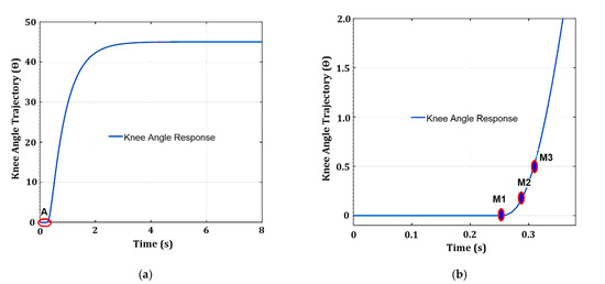
Figure 8.
Extraction of time delay using a three-point (M1, M2, and M3) moving average method from knee angle response. (a) knee angle response with a time delay at point A; (b) zoomed view into the marked area A of the knee angle response with a three-point average (M1, M2, and M3).
The time delay is calculated for every new patient in real time. This value is used to determine the types of FCUs to be used. The SM FCU is used for small time delays (0–0.06 s). For moderate time delays (0.07–0.13 s), the USM FCU unit is used. For high-time delays (above 0.26 s), the USM FCU with DTC is used. The results section explains detailed analyses and justifications for using SM or USM FCU according to the time delay duration.
- 2.
- Extraction of Rise Time from Knee Angle Response
In this work, during the open-loop stimulation, the knee torque output is set to operate at a target angle of 45°. Figure 9 illustrates the extraction of the rise time from the acquired knee angle trajectory response using an internal counter. Once the FES open loop system starts to operate, the internal counter is activated when the acquired knee angle is at 10% (4.5°) of the target angle (45°). The counter stops counting when the acquired knee angle reaches 90% (40.5°) of the target angle (45°). Therefore, once the acquired knee angle reaches a value of 40.5°, the internal counter stops counting, and the rise time is calculated by multiplying the counted value by its time interval (0.01 s). The calculated rise time is 1.21 s (121 counted values × 0.01 s).
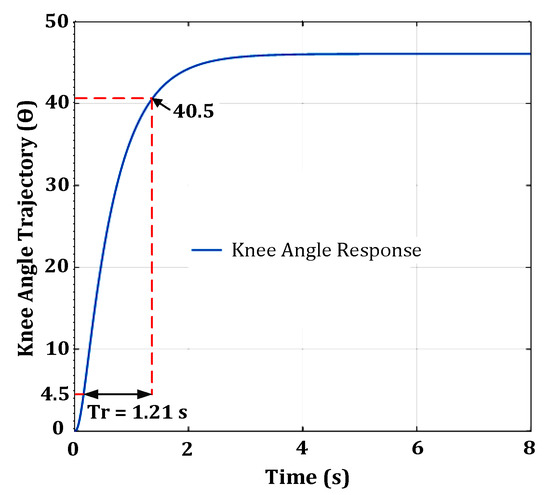
Figure 9.
Extraction of rise time using an internal counter from the knee angle response.
The calculated rise time is used to determine the suitable reference angle and the SM gain for that patient. A smaller SM gain will be required for a fast rise time, and a higher SM gain will be required for a slow rise time.
- 3.
- Extraction of Overshoot from Knee Angle Response
The overshoot is calculated by subtracting the steady-state value from the maximum peak value, as depicted in Figure 10a and shown in Equation (63). The maximum peak value is calculated using the three-point (M1, M2, and M3) moving average method, as shown in Figure 10b in the zoomed view. The peak point is determined when M2 is greater than M1 and M3, as illustrated in Figure 10b. The calculated overshoot value is used to determine a suitable SM gain setting during the closed-loop operation. When an overshoot occurs, a lower SM gain setting will be used.
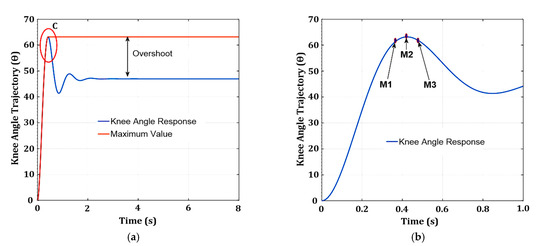
Figure 10.
Extraction of overshoot using a three-point (M1, M2, and M3) moving average method from the knee angle response: (a) knee angle response with overshoot; (b) zoomed view into marked area C of knee angle response with the three-point (M1, M2, and M3) moving average.
- 4.
- Extraction of Steady State Value, Error, and Time
The steady-state value is extracted using the three-point (M1, M2, and M3) moving average method, as illustrated in Figure 11. The three points (M1, M2, and M3) are separated by 0.05 ms, as shown in the zoomed view in Figure 11b. The steady-state value is extracted after the system passes the time delay calculation and the internal counter value is above 50. The steady-state value is determined when the three-point (M1, M2, and M3) values are almost similar and the differences among the three are less than 0.1. The steady-state value is used to determine the suitable reference angle setting for the system. Once the steady-state value is known, Equation (64) determines the steady-state error by subtracting the steady-state value from the reference angle.
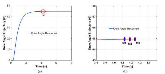
Figure 11.
Extraction of steady-state value, error, and time using a three-point (M1, M2, and M3) moving average method from the knee angle response: (a) knee angle response with steady-state value at point B; (b) zoomed view into marked area B of the knee angle response with the three-point average (M1, M2, and M3).
Additionally, when the system reaches its steady-state value, the steady-state time is found by multiplying the counted value of the internal counter by the time interval of the counter delay (0.01 s), as shown in Equation (65).
After determining the steady-state value, error, and time, the closed-loop system can operate with the relevant reference angle setting.
- 5.
- Detection of Stiffness, Fatigue, and Spasticity from Knee Angle Response
The stiffness, spasticity, and fatigue are detected by transforming the acquired knee angle response into a rate of change response. The rate of change response is obtained by subtracting the previously acquired knee angle data from the current knee angle data. For stiffness and spasticity, the internal minimum and maximum counters and the three-point (M1, M2, and M3) moving average method are used to determine the number of maximum and minimum peaks from the knee angle rate of change response. The three-point (M1, M2, and M3) moving average method determines the maximum or minimum value. The maximum peak point is determined when M2 is greater than M1 and M3. The minimum peak point is determined when M2 is smaller than M1 and M3. The maximum counter is increased whenever there is a maximum peak, and the minimum counter is increased whenever there is a minimum peak. As depicted in Figure 12a, for a normal knee angle response (without any nonlinearities), the rate of change has only one maximum peak value. When the knee angle rate of change response has two maximum peaks with one minimum peak in between, stiffness is detected, as illustrated in Figure 12b. However, spasticity is detected when the knee angle rate of change response has several maximum and minimum peaks, as shown in Figure 12c. Figure 12d shows that the knee angle rate of change response is less than zero when fatigue is present.
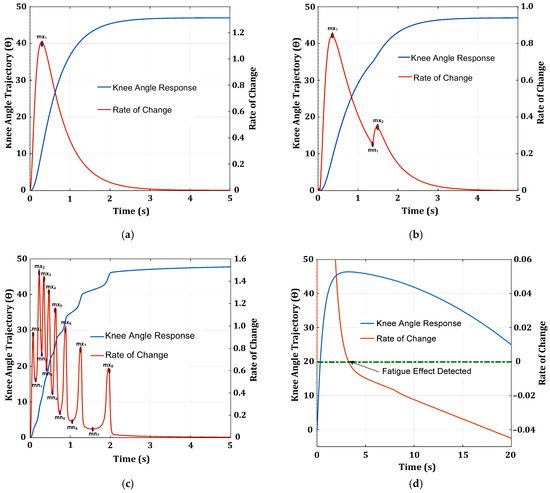
Figure 12.
Detection with and without nonlinearities from the knee angle response: (a) knee angle response without nonlinearities; (b) knee angle response with stiffness; (c) knee angle response with spasticity; (d) knee angle response with fatigue.
2.6.2. Tunable Feedback Control Unit (SM/USM)
The function of the tunable feedback control unit (SM or USM) is to provide an accurate amount of charge (pulse width) to stimulate the quadricep muscles for knee angle movement. Two types of FCUs, SM and USM, were designed for the adaptive feedback controller. These FCUs were designed to be tunable in real time or online in response to muscle nonlinearities, disturbances, and system changes. After the system identification process, the main control unit determines the appropriate gain, reference angle, and control law settings for the FCUs (SM and USM) according to the status of the patient under treatment. Based on the selected gain, reference angle, and control laws, the FCU (SM or USM) calculates the appropriate control output (Ctrlout) or stimulus pulse width that needs to be provided for stimulation purposes. If the system has a time delay, the main control unit activates the USM FCU when the time delay is above 0.05 s and turns on DTC (for time delays above 0.26 s) to reduce the oscillating effect of the time delay.
2.6.3. Direct Torque Control (DTC) for Time Delay System
DTC is used to deal with the system’s time delay problem in this adaptive feedback controller design. According to previous research [11], as the system’s time delay increases, the feedback controller system begins to oscillate and becomes unstable [64], and overshoots will also increase [10,11,30]. Therefore, when the time delay is calculated to be above 260 ms, DTC is activated to operate together with the USM FCU. DTC works very well when associated with the USM FCU.
The DTC technique changes the control reference, originally based on the reference angle, into an equivalent torque, as shown in Figure 13. The converted equivalent torque has a smaller value compared with the knee angle. Therefore, the calculated error between the reference and actual angles is much smaller when the equivalent torque conversion values are used. These small errors keep the controller from acting quickly and roughly because it works at lower error rates. Hence, the DTC techniques prevent the controller from reaching its maximum output, which keeps it from oscillating [71].
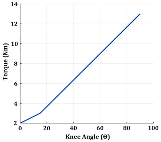
Figure 13.
Angle to torque conversion look-up table (LUT) for direct torque control (DTC).
3. Results
This section discusses the performance of the three FCUs (SM, PID, and FL) when tested with and without nonlinearities (fatigue, time delay, stiffness, and spasticity). In this work, because the SM feedback control unit exhibited the best performance compared with PID and FL, SM was used for the adaptive feedback controller implementation. The performance of the adaptive SM feedback control algorithm tested with the nonlinear knee model is also discussed.
3.1. Three Feedback Control Units Performance Using Optimized Gain
This section discusses the simulation results of three FCUs (SM, PID, and FL) tested on a knee model with and without nonlinearities.
3.1.1. Knee Model without Nonlinearities
Figure 14 depicts the knee angle response at four reference angles (20°, 30°, 40°, and 76°) without nonlinearity and with fatigue nonlinearity for three FCUs (SM, PID, and FL). Figure 14a,c,e shows the knee angle responses of the SM, PID, and FL FCUs in the absence of any nonlinearity. Although the FCUs tuning was conducted only at 40°, all FCUs observed could meet the target angles except for FL, which exhibits the largest steady-state error at a reference angle of 76°. The PID feedback control unit has a smooth knee angle response at all reference angles.
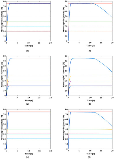
Figure 14.
Knee angle response without nonlinearities and with fatigue nonlinearity using three FCUs (SM, PID, and FL): (a) knee angle response without nonlinearities for SM; (b) knee angle response with fatigue for SM; (c) knee angle response without nonlinearities for PID; (d) knee angle response with fatigue for PID; (e) knee angle response without nonlinearities for FL; (f) knee angle response with fatigue for FL. The reference angle (ref) and knee response (resp) are represented in different coloured lines as follows: (i) ref 76°: orange and resp: blue; (ii) ref 40°: light green and resp: yellow; (iii) ref 30°: light blue and resp: purple; (iv) ref 20°: red and resp: blue.
The key performance parameters of the three FCUs (SM, PID, and FL), which include rise time, settling time, overshoot, and steady-state error at four reference angles (20°, 30°, 40°, and 76°), are tabulated in Table 5. The tabulated results show that the rise time and settling time for the three FCUs (SM, PID, and FL) increase as the reference angles increase. The rise time and settling time for SM and FL are almost the same across all reference angles. PID is observed to have the highest values for rise time and settling time among the three FCUs across all reference angles. The overshoot for SM and FL is more pronounced at lower reference angles (20°, 30°, and 40°) and less so at a higher reference angle (76°). The steady-state error of FL is the highest (1.688°) among the three FCUs at a higher reference angle (76°).
Table 5.
FCU (SM, PID, and FL) performance (rise time, settling time, overshoot, and steady-state error) tested on the knee model (without nonlinearities) at four reference angles (20°, 30°, 40°, and 76°).
3.1.2. Knee Model with Fatigue Nonlinearity
When fatigue is incorporated into the knee model, as depicted in Figure 14b,d,f, the FCUs (SM, PID, and FL) maintain their performance at lower reference angles (20°, 30°, and 40°). However, the performance of the FCUs (SM, PID, and FL) starts to degrade around 12 s for the higher reference angle of 76°. At around 12 s, the performance of all FCUs (SM, PID, and FL) starts to decline, and the knee angle trajectories begin to drop significantly. Muscle fatigue results in small oscillations in the knee angle trajectory response for the SM FCU before the knee drops. The drop in knee angle trajectory after 12 s indicates that muscle fatigue significantly affects the knee angle trajectory at a higher reference angle (76°). Consequently, the steady-state error increases substantially after 12 s, reaching a value around 30° (76° − 46° = 30°) at the reference angle of 76°, as shown in Figure 14b,d,f. The steady-state error of FL is still the highest among the three FCUs across all times, at a reference angle of 76°.
3.1.3. Knee Model with Stiffness Nonlinearity
The knee angle responses of three FCUs (SM, PID, and FL) with stiffness at four different reference angles (20°, 30°, 40°, and 76°) are shown in Figure 15a,c,e. It is observed that the SM FCU is robust and immune to the effect of stiffness because the knee responses are quite stable, with minimal steady-state errors (0.1° to 0.2°) at all reference angles. For the PID FCU, the stiffness effect causes overshoot around the value of 1° to 1.8° in the knee response, especially at lower reference angles (20°, 30°, and 40°). For FL FCU, the stiffness does not affect the knee response and still has a similar large steady-state error (1.69°) at a higher reference angle (76°). This is expected as the FL controller has a lower control bandwidth [30,31].
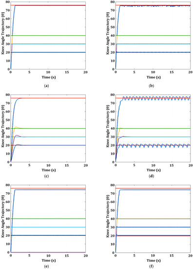
Figure 15.
Knee angle response with stiffness and spasticity using three FCUs (SM, PID, and FL): (a) knee angle response with stiffness for SM; (b) knee angle response with spasticity for SM; (c) knee angle response with stiffness for PID; (d) knee angle response with spasticity for PID; (e) knee angle response with stiffness for FL; (f) knee angle response with spasticity for FL. The reference angle (ref) and knee response (resp) are represented in different coloured lines as follows: (i) ref 76°: orange and resp: blue; (ii) ref 40°: light green and resp: yellow; (iii) ref 30°: light blue and resp: purple; (iv) ref 20°: red and resp: blue.
3.1.4. Knee Model with Spasticity Nonlinearity
The knee angle responses for the three FCUs (SM, PID, and FL) with spasticity at four different reference angles (20°, 30°, 40°, and 76°) are shown in Figure 15b,d,f. For SM and PID FCUs, the spasticity effect causes the knee response to oscillate at reference angles of 20° and 76°. The oscillation of the knee response for PID FCU is more prominent and more significant compared with the SM FCU at the lower reference angle (20°) and the higher reference angle (76°). The oscillation of the knee response for the SM FCU increases at a higher reference angle (76°). The knee response for the FL FCU is not affected much by the spasticity effect, except for small overshoots (0.4° to 0.5°) at lower reference angles (20° and 30°). The steady-state error of the FL FCU is still high (1.69°) at the reference angle of 76°. The PID FCU exhibits the worst performance, with a significant oscillation of knee response at smaller and higher reference angles (20° and 76°). PID FCU has the highest steady-state error (4°) at smaller and higher reference angles (20° and 76°). From the knee-angle trajectory oscillating response behaviour, it is observed that SM and PID controllers cannot compensate for the effect of spasticity, especially at smaller and higher reference angles (20° and 76°). FL FCU is found to be robust to the nonlinear spasticity effect.
3.1.5. Knee Model with Time Delay (10 ms, and 260 ms) Nonlinearity
The knee angle responses of three FCUs (SM, PID, and FL) with a time delay of 10 ms at four different reference angles (20°, 30°, 40°, and 76°) are shown in Figure 16a,c,e. The knee response for the PID FCU seems relatively smooth, with no oscillation at any reference angles. The time delay causes small oscillations at all reference angles for the SM FCU. However, for the FL FCU, the time delay of 10 ms has a higher oscillation when compared with the SM FCU.
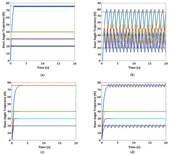
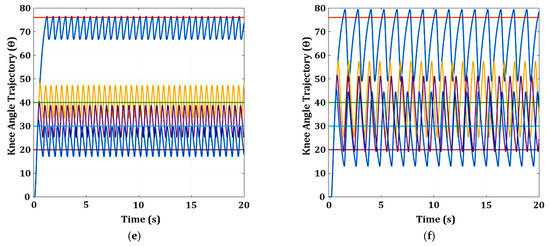
Figure 16.
Knee angle response with time delay 10 ms and 260 ms using three FCUs (SM, PID, and FL): (a) knee angle response with a time delay of 10ms for SM; (b) knee angle response with a time delay of 260 ms for SM; (c) knee angle response with a time delay of 10 ms for PID; (d) knee angle response with time a delay of 260 ms for PID; (e) knee angle response with a time delay of 10 ms for FL; (f) knee angle response with a time delay of 260 ms for FL. The reference angle (ref) and knee response (resp) are represented in different coloured lines as follows: (i) ref 76°: orange and resp: blue; (ii) ref 40°: light green and resp: yellow; (iii) ref 30°: light blue and resp: purple; (iv) ref 20°: red and resp: blue.
The knee angle responses of three FCUs (SM, PID, and FL) with a time delay of 260 ms at four different reference angles (20°, 30°, 40°, and 76°) are shown in Figure 16b,d,f. The large time delay (260 ms) causes bigger oscillations in the knee response for SM and FL FCUs at all reference angles. It is observed that the SM and FL FCUs could not eliminate the time delay effect at all reference angles and had a degraded closed-loop performance. SM FCU has the highest overshoot and steady-state errors in the range of 15° to 24° at all reference angles (20°, 30°, 40°, and 76°). FL FCU has the second-highest overshoot and steady-state errors in the range of 2° to 22° at all reference angles (20°, 30°, 40°, and 76°). The knee response for PID FCU also shows small oscillations at reference angles of 20° and 76°.
3.1.6. Knee Model with Time Delay Nonlinearity Using DTC (260 ms)
To overcome heavy oscillation in the knee response when a higher time delay exists in the system, DTC was employed in all FCUs (SM, PID, and FL). Additionally, to reduce the significant effect of chattering in the SM at a higher time delay, the SM was replaced with a USM FCU. The knee angle response with a time delay of 260 ms is shown in Figure 17a when USM FCU is used. The heavy oscillation is significantly reduced compared with the SM FCU (as shown in Figure 16b).
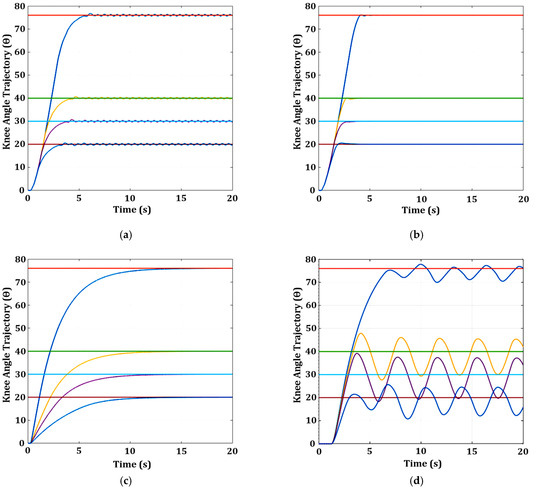
Figure 17.
Knee angle response with a 260 ms time delay using three FCUs (USM, PID, and FL): (a) knee angle response with a time delay of 260 ms for USM; (b) knee angle response with a 260 ms time delay for USM with DTC; (c) knee angle response with a 260 ms time delay for PID with DTC; (d) knee angle response with a 260 ms time delay for FL with DTC. The reference angle (ref) and knee response (resp) are represented in different coloured lines as follows: (i) ref 76°: orange and resp: blue; (ii) ref 40°: light green and resp: yellow; (iii) ref 30°: light blue and resp: purple; (iv) ref 20°: red and resp: blue.
Figure 17b–d depicts the knee angle response for the three FCUs (USM, PID, and FL) with DTC activation for a 260 ms time delay at four different reference angles (20°, 30°, 40°, and 76°). It is observed that the knee response of USM FCU with DTC (Figure 17b) activation is relatively smooth at four reference angles (20°, 30°, 40°, and 76°) when a time delay of 260 ms exists in the system. As shown in Table 6, USM FCU with DTC activation has a much faster rise time at a lower reference angle (20° and 30°) than the USM FCU operating alone. Although the PID FCU with DTC (Figure 17c) has a smooth knee response (no oscillation), the rise time at all reference angles is quite large (ranging from 5.26 s to 6.42 s) when compared with the PID FCU that operates alone (shown in Figure 16d). The knee response for the FL FCU with DTC (Figure 17d) still oscillates. However, the knee response has shown some reduction in the oscillation amplitude and frequency at four reference angles (20°, 30°, 40°, and 76°) with an increment in the rise time value when compared with the FL FCU that operates alone (shown in Figure 16f).
Table 6.
Rise time for USM, USM with DTC, PID with DTC, and FLC with DTC for the knee extension model with a time delay of 260 ms.
From the results of all the knee response simulations, USM FCU with DTC works best when the time delay in the system is high.
3.1.7. Knee Model with Disturbance Nonlinearity
To evaluate the performance of the tested FCUs against the internal and external disturbances, the knee model was further injected with a sinusoidal signal that emulated other disturbances from internal muscle and external forces, as depicted in Figure 18a. The internal disturbance represents the mismatch model, dynamic uncertainties, and changes in dynamic parameters such as shank weight, shank length, and damping effect variations. The knee angle responses for the three FCUs (SM, PID, and FL) with signal disturbances are shown in Figure 18b,c,d at four reference angles (20°, 30°, 40°, and 76°). SM exhibits minimal oscillations at four reference angles (20°, 30°, 40°, and 76°), as shown in Figure 18b. FL is also observed to have minimal oscillations at four reference angles (20°, 30°, 40°, and 76°). However, the steady-state error still exists at the higher reference angle (76°), as depicted in Figure 18d. PID is observed to exhibit the most prominent oscillations among the three FCUs at four reference angles (20°, 30°, 40°, and 76°), as depicted in Figure 18c. As listed in Table 7, PID has the highest overshoot (2.02°) and steady-state errors (2.4° to 3.6°) among the three FCUs. Based on the simulation results, SM FCU performed better than the PID and FL FCUs at all reference angles (20°, 30°, 40°, and 76°) in terms of robustness against signal disturbances.
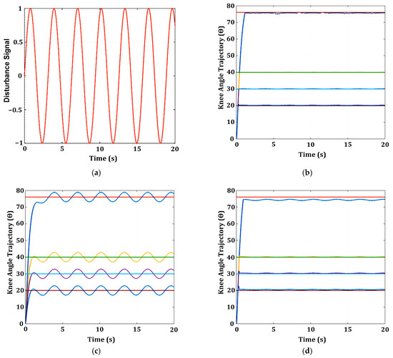
Figure 18.
Knee angle response with disturbance using three feedback controllers (SM, PID, and FL): (a) sinusoidal signal as disturbance; (b) knee angle response with disturbance for SM; (c) knee angle response with disturbance for PID; (d) knee angle response with disturbance for FL. The reference angle (ref) and knee response (resp) are represented in different coloured lines as follows: (i) ref 76°: orange and resp: blue; (ii) ref 40°: light green and resp: yellow; (iii) ref 30°: light blue and resp: purple; (iv) ref 20°: red and resp: blue.
Table 7.
FCU (SM, PID, and FL) performance (rise time, settling time, overshoot, and steady-state error) tested on a nonlinear knee model (disturbance) at four reference angles (20°, 30°, 40°, and 76°).
3.1.8. Summary of Performance Analyses for Three Feedback Control Units
This section summarises the overall findings of the three FCUs (SMC, PID, and FL) that led to the final decision to select the best FCU among the three.
For the knee extension model without any nonlinearity, all three FCUs (SM, PID, and FL) were able to perform and track the four reference angles (20°, 30°, 40°, and 76°), except for FL, which has a sizeable steady-state error (1.69°) at the reference angle of 76°. When the fatigue nonlinearity element was introduced into the knee model, the three FCUs could only maintain their performance when tracking the small ranges of reference angles (20°, 30°, and 40°). At a higher reference angle (76°), the three FCUs could no longer track the reference angle at 13 s, where the FCUs’ performance started to degrade, and the knee angle started to drop. The drop in the knee angle trajectory implied that muscle fatigue significantly affects the knee trajectory at the higher reference angle (76°).
When stiffness was incorporated into the knee model, all three FCUs were observed to be immune and robust against stiffness nonlinearity. Only the PID FCU had a little bit of overshoot (1° to 1.8°), especially at lower reference angles (20°, 30°, and 40°). The FL was also observed to be immune and robust against stiffness, except that it still had a sizeable steady-state error (1.69°) at the higher reference angle (76°). The performance of the three FCUs (SM, PID, and FL) was also observed when the knee extension model was incorporated with spasticity at the four reference angles (20°, 30°, 40°, and 76°). The spasticity affected the SM and PID FCUs, which caused the knee response to oscillate, especially at the smaller and higher reference angle (20° and 76°, respectively). The oscillation of the knee response in PID was higher than in SM FCU. FL FCU was resistant to the nonlinear spasticity effect, except for having a steady-state error of 1.69° at a higher reference angle (76°).
When the knee model was incorporated with a larger time delay (260 ms), heavy oscillations were observed in the knee responses of SM and FL FCUs. The controllers could not eliminate the time delay effect at all reference angles and had a poor closed-loop performance. To overcome the SM chattering effect on the knee angle response when a larger time delay exists in the system, an unchattered SM FCU was introduced. Therefore, the chattering SM was replaced with the unchattering SM (USM) when a more prolonged time delay (>0.05 s) was detected. Additionally, a DTC was employed in the feedback controller to remove the oscillatory effect. The USM FCU and DTC were activated when the time delay was equal to or above 0.26 s. The performance was improved, and heavy oscillation in the knee response was tremendously reduced when the USM FCU with DTC was employed. The knee response of the USM FCU with DTC showed smooth tracking at all four reference angles (20°, 30°, 40°, and 76°) when a higher time delay (>0.26 s) existed in the system.
The three FCUs (SM, PID, and FL) were also tested with a knee model with disturbance nonlinearity, representing the mismatch model, dynamic uncertainties, and changes in dynamics parameters such as shank weight, shank length, and damping effect variations. The controllers were observed to have oscillations in the knee response at four reference angles (20°, 30°, 40°, and 76°). PID FCU had the most prominent oscillations and the highest overshoot and steady-state errors compared to the other two FCUs. The SM and FL showed the smallest oscillations at all reference angles. However, FL still had a high steady-state error at a higher reference angle (76°). Among the three controllers, SM FCU demonstrated the best performance with minimal oscillations and robustness against the disturbances at all reference angles.
After evaluating the three FCUs’ performances with the nonlinear knee model, the SM FCU was observed to exhibit the best performance at four reference angles (20°, 30°, 40°, and 76°) among the three FCUs. In general, the SM and FL FCUs were observed to demonstrate relatively small rise time, settling time, overshoot, and steady-state error at low reference angles (20°, 30°, and 40°), compared with PID. However, at a higher reference angle (76°), SM FCU performed better than the FL FCU by having the smallest overshoot and steady-state error. When nonlinear disturbances were incorporated into the knee model, SM FCU was observed to be robust by having the smallest steady-state error and overshoot among the three FCUs. Additionally, by modifying the SM into a USM and coupling it with DTC, it was observed that the USM FCU could also eliminate heavy oscillation in the knee response when a larger time delay (0.26 s) existed in the system.
Therefore, SM FCU was used to implement the adaptive SM feedback controller with a system identification feature and a tunable internal FCU (SM or USM) to provide an accurate stimulus charge according to the patient’s condition. The system identification unit was used to extract essential features (rise time, overshoot, and steady-state error) of the knee response and to detect the knee model’s nonlinear element (time delay, fatigue, stiffness, and spasticity). Based on the output results obtained from the system identification unit, the gain and control laws for the tunable internal FCU (SM or USM) were adjusted accordingly.
3.2. Adaptive Sliding Mode Feedback Controller
The previous section’s simulation results show that SM FCU exhibited the best performance compared with PID and FL. Therefore, SM FCU was used to implement the adaptive feedback controller. As mentioned in the previous section, the adaptive SM feedback control algorithm was designed with a system identification feature that could identify the condition of the patient under treatment and fine-tune the internal FCU settings (gain, reference angle, and control laws) to adapt and provide accurate stimulus charges according to the patient’s current condition. The operation of the FES system using the adaptive SM feedback control algorithm starts with open-loop stimulation to identify the patient’s condition, followed by closed-loop operation.
This section discusses the simulation results of the adaptive SM feedback controller with the nonlinear knee extension model. The performance of the adaptive SM feedback control algorithm was evaluated at several knee model nonlinearities, which include low muscle torque output, a large time delay (260 ms), fatigue, stiffness, spasticity, and other disturbances. Additionally, the performance of the adaptive SM feedback controller was compared with the conventional SM feedback controller and other previous research for analysis purposes.
3.2.1. Knee Model with Low-Power Muscle Torque
This section discusses the results of low muscle torque output, which mimics the condition of SCI patients in early rehabilitation exercises [72]. Figure 19 depicts the knee angle responses for the conventional SM feedback controller (Figure 19a) and the adaptive SM feedback controller (Figure 19b) when the muscle torque output is low. From the simulation results, it is observed that, for the conventional SM feedback controller, the fixed reference angle of 45° caused the knee response to decline around 3 s due to low muscle torque output, which could not meet the target angle. For the adaptive SM feedback controller, after the system identification process during open-loop stimulation, the main control unit set a suitable reference angle of 13°, as depicted in Figure 19b. Thus, the knee response could meet the newly set target angle with a minimal steady-state error. The closed-loop FES was observed to maintain the knee at a 13° angle for up to 7 s before the knee started to fatigue and drop.
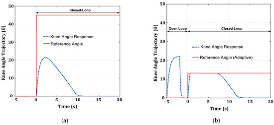
Figure 19.
Knee angle response with low power muscle torque for conventional SM and adaptive SM feedback controllers: (a) knee angle response with low power muscle torque for the conventional SM feedback controller; (b) knee angle response with low power muscle torque for the adaptive SM feedback controller.
Table 8 lists the conventional and adaptive SM feedback controllers’ settling time, drop time, and knee extension duration. The knee extension duration is calculated by subtracting the settling time from the drop time. The calculated knee duration for the conventional SM feedback controller is 1 s, while the knee duration for the adaptive SM feedback controller is 6 s. Therefore, the improvement in the knee extension duration by the adaptive SM feedback controller is 83% compared with the conventional feedback controller.
Table 8.
Conventional and adaptive SM feedback controller performance tested on low power muscle torque at a reference angle of 45°.
3.2.2. Knee Model with Time Delay (260 ms) Nonlinearity
Figure 20 depicts the knee angle response with a time delay of 260 ms included in the knee model for the conventional SM feedback controller (Figure 20a), adaptive SM feedback controller (Figure 20b), adaptive USM feedback controller (Figure 20c), and adaptive USM feedback controller with DTC (Figure 20d). The simulation results show that the knee response oscillates significantly throughout the entire time at a reference angle set at 45° for the conventional SM feedback controller (Figure 20a). For the adaptive SM feedback controller (Figure 20b), the knee response also oscillates heavily throughout the entire time during the closed-loop operation. The oscillation of the knee response is reduced to a smaller value when the adaptive USM feedback controller is used, as shown in Figure 20c. However, when the adaptive USM feedback controller is combined with DTC, the oscillation of the knee angle response is eliminated, as shown in Figure 20d. Therefore, when the time delay is high (260 ms), the best option for the adaptive feedback controller is to use USM with DTC to ensure stability and avoid oscillation in the knee response.
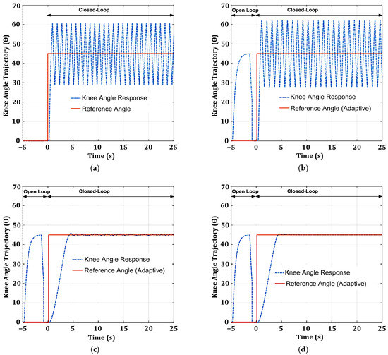
Figure 20.
Knee angle response with a 260 ms time delay for conventional SM and adaptive SM feedback controllers: (a) knee angle response with a 260 ms time delay for the conventional SM feedback controller; (b) knee angle response with a 260 ms time delay for the adaptive SM feedback controller; (c) knee angle response with a 260 ms time delay for the adaptive USM feedback controller; (d) knee angle response with a 260 ms time delay for the adaptive USM feedback controller and DTC.
As listed in Table 9, the conventional SM feedback controller has a higher overshoot (±15°) and steady-state error (14.38°) compared with the adaptive USM feedback controller with DCT, which has no overshoot and a minimal steady-state error (0.44°). However, the USM feedback controller with DTC has a higher rise time (2.71 s) and settling time (4.03 s) than the conventional SM feedback controller. The higher rise time and settling times produced by the adaptive USM with DTC are still acceptable for stimulation operations as they occur at the beginning of the knee exercise and are not critical. The essential parameters are overshoot, steady error, and oscillation. Heavy oscillation in the knee response indicates instability in the controller. Therefore, the adaptive USM with DTC performed better than conventional SM by having a 100% reduction in overshoot and a 96.9% reduction in steady-state error. Additionally, oscillation was also eliminated from the system.
Table 9.
Conventional SM and adaptive USM feedback controller performance (rise time, settling time, overshoot, and steady-state error) was tested on a nonlinear knee model (time delay = 260 ms) at a reference angle of 45°.
3.2.3. Knee Model with Fatigue Nonlinearity
Figure 21a depicts the knee response of the conventional SM feedback controller with mild fatigue at a reference angle of 45°. The simulation result shows that at 32 s, the knee starts to fatigue and drops drastically to 0° from the reference angle (45°). As a result, the duration of an FES rehabilitation exercise is around 32 s for the conventional SM feedback controller. Figure 21b depicts the knee response of the adaptive SM feedback controller with mild fatigue at a 45° reference angle. As the adaptive feedback controller was designed with the capability to detect fatigue, the controller is adjusted to a lower reference angle value (35°) when fatigue is detected at around 22 s. The adaptive feedback controller then maintains its reference angle of 35° until the second fatigue is detected at around 44 s. At this point, the controller reduces its reference angle to another lower value of 25°. The adaptive feedback controller then maintains its reference angle of 25° until the third fatigue is detected at around 66 s. The controller reduces its reference angle to another lower value of 15°. Finally, when the fifth fatigue is detected at 74 s, the knee response drops drastically to 0°. The knee can no longer follow the newly set reference angle of 15° around 74 s. The total duration of the closed-loop FES operation is around 74 s. As a result, the total knee extension duration of adaptive SM feedback controller operation is greater than that of the conventional SM feedback controller operation. The overall duration for the adaptive SM feedback controller to maintain the knee response at the dynamically adaptive target angle according to muscle fatigue conditions is greater than that of the conventional SM feedback controller by 131%.
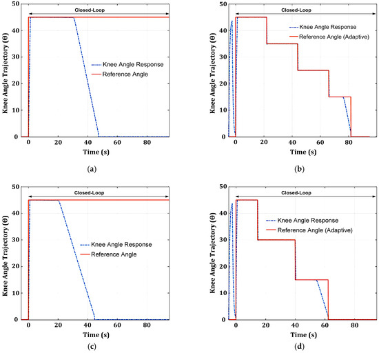
Figure 21.
Knee angle response with fatigue for conventional SM and adaptive SM feedback controllers: (a) knee angle response with mild fatigue for the conventional SM feedback controller; (b) knee angle response with mild fatigue for the adaptive SM feedback controller; (c) knee angle response with severe fatigue for the conventional SM feedback controller; (d) knee angle response with severe fatigue for the adaptive SM feedback controller.
Figure 21c depicts the knee response of the conventional SM feedback controller with severe fatigue at a reference angle of 45°. The simulation result shows that at 20 s, the knee starts to fatigue and drops drastically to 0° from the reference angle (45°). As a result, the duration of an FES rehabilitation exercise is around 20 s for the conventional SM feedback controller. Figure 21d depicts the knee response of the adaptive SM feedback controller with severe fatigue at a 45° reference angle. As the adaptive feedback controller was designed with the capability to detect fatigue, the controller is adjusted to a lower reference angle value (30°) when fatigue is detected at around 17 s. The adaptive feedback controller then maintains its reference angle of 30° until the second fatigue is detected at around 40 s. At this point, the controller reduces its reference angle to another lower value of 15°. The adaptive feedback controller then maintains its reference angle of 15° until the third fatigue is detected at around 54 s. Finally, when the fifth fatigue is detected at 54 s, the knee response drops drastically to 0°. The knee can no longer follow the newly set reference angle of 15° at around 54 s. The total duration of the closed-loop FES operation is around 54 s. As a result, the total duration of the adaptive SM feedback controller operation is greater than that of the conventional SM feedback controller operation. The overall duration for the adaptive SM feedback controller to maintain the knee response at the dynamically adaptive target angle according to muscle fatigue conditions is greater than that of the conventional SM feedback controller by 170%.
Table 10 summarises the duration of the knee angle response for the conventional and adaptive SM feedback controllers with mild and severe fatigue incorporated into the knee model. The conventional SM feedback controller employed a fixed reference angle (45 °), while the adaptive SM feedback controller employed an adaptive reference angle throughout the exercise duration. For mild fatigue, the conventional SM feedback controller could only operate for up to 32 s, while the adaptive SM feedback controller could operate for up to 74 s. The adaptive SM feedback controller is observed to have a 42 s prolongation time that accounts for 131% improvement compared with the conventional SM feedback controller. For severe fatigue, the conventional SM feedback controller could only operate for up to 20 s, while the adaptive SM feedback controller could operate for up to 54 s. The adaptive SM feedback controller is observed to have a 34 s prolongation time, which accounts for a 170% improvement compared with the conventional SM feedback controller. The results prove that the adaptive SM feedback controller could prolong the knee extension exercise by changing the reference angle to a lower value that suited the muscle torque output once fatigue was detected.
Table 10.
Conventional and adaptive SM feedback controller performance tested on a nonlinear knee model (fatigue) at a reference angle of 45°.
3.2.4. Knee Model with Stiffness Nonlinearity
Figure 22 depicts the knee response for the conventional SM (Figure 22a) and adaptive SM feedback (Figure 22b) controllers when the knee model has stiffness. It is observed that both conventional and adaptive SM feedback controllers could compensate for the nonlinear stiffness effect in the knee model. The knee angle responses for both controllers are smooth, with no chattering, and are capable of meeting the target angle.
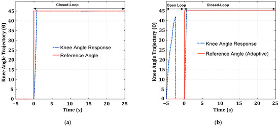
Figure 22.
Knee angle response with stiffness for conventional SM and adaptive SM feedback controllers: (a) knee angle response with stiffness for the conventional SM feedback controller; (b) knee angle response with stiffness for the adaptive SM feedback controller.
3.2.5. Knee Model with Spasticity Nonlinearity
Figure 23a depicts the knee response for the conventional SM feedback controller with spasticity in the knee model at a reference angle of 45°. The knee angle response is seen to have small oscillations throughout the entire duration. Figure 23b depicts the adaptive SM feedback controller’s knee response when spasticity exists in the knee model at a reference angle of 45°. In the adaptive SM feedback controller, the gain is adjusted to compensate for the effect of chattering in the knee response during the closed-loop operation. The knee response was relatively smooth and could maintain a minimal steady-state error throughout the operation. Table 11 shows that the conventional SM and adaptive feedback controllers have comparatively similar values of rise time, settling time, overshoot, and steady-state error. However, the adaptive SM feedback controller has a smooth knee response compared with the conventional SM feedback controller, which has a small oscillation in the knee response.
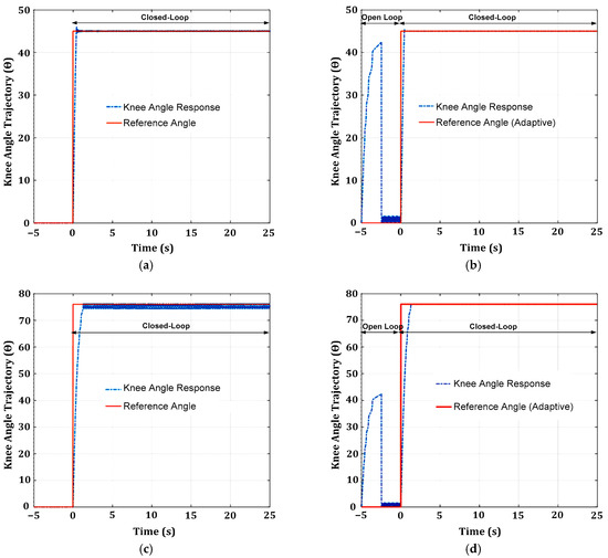
Figure 23.
Knee angle response with spasticity for conventional SM and adaptive SM feedback controllers: (a) knee angle response with spasticity for the conventional SM feedback controller at a ref. angle of 45°; (b) knee angle response with spasticity for the adaptive SM feedback controller at a ref. angle of 45°; (c) knee angle response with spasticity for the conventional SM feedback controller at a ref. angle of 76°; (d) knee angle response with spasticity for the adaptive SM feedback controller at a ref. angle of 76°.
Table 11.
Conventional and adaptive SM feedback controller performance (rise time, settling time, overshoot, and steady-state error) was tested on a nonlinear knee model (spasticity) at two reference angles (45° and 76°).
Figure 23c shows the knee response for the conventional SM feedback controller with spasticity in the knee model at a reference angle of 76°. The knee angle response oscillates throughout the duration and has a higher rise time (0.92 s), as listed in Table 11. Figure 23d depicts the adaptive SM feedback controller’s knee response when spasticity exists in the knee model at a reference angle of 76°. The reference angle was purposely increased to a higher value of 76° (regardless of the open-loop steady state value) to observe the adaptive SM feedback controller’s performance at a higher reference angle. The gain was adjusted to compensate for the oscillation effect in the knee response of the adaptive SM feedback controller. The knee response was relatively smooth and could maintain a small steady-state error throughout the operation, as shown in Figure 23d, compared with the conventional SM feedback controller. As listed in Table 11, at a higher reference angle (76°), the overshoot and steady-state error for the adaptive SM feedback controller has been reduced tremendously to a lower value of 0.06° compared with the conventional SM feedback controller. Therefore, the adaptive SM feedback controller performed better than conventional SM by having a 94% reduction in overshoot and a 97% reduction in steady-state error.
3.2.6. Knee Model with Disturbance Nonlinearity
Figure 24 depicts the knee response for the conventional and adaptive SM feedback controllers with nonlinear disturbance in the knee model at four reference angles (20°, 30°, 40°, and 76°). Figure 24a depicts the conventional SM feedback controller’s knee angle responses with nonlinear disturbances. The knee angle responses exhibit small oscillations at the four reference angles (20°, 30°, 40°, and 76°). Figure 24b depicts the adaptive SM feedback controller’s knee angle responses to nonlinear disturbances. The knee angle responses are quite smooth and stable, and could compensate for the effect of nonlinear disturbances by having short rise and settling times, small overshoots, and small steady-state errors and could still track the four reference angles (20°, 30°, 40°, and 76°), although the tuning was conducted at a reference angle of only 40°. Table 12 indicates that the conventional SM and adaptive feedback controllers have almost similar values for rise time, settling time, overshoot, and steady-state error at lower reference angles (20°, 30°, and 40°). However, at higher reference angle (76°), the adaptive SM feedback controller performs better than the conventional SM feedback controller by having a 19% reduction in rise time, a 20% reduction in settling time, and a 93% reduction in steady-state error.
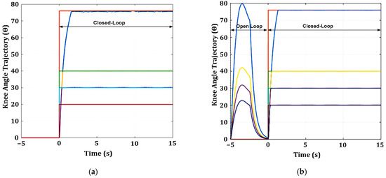
Figure 24.
Knee angle response with disturbance for conventional SM and adaptive SM feedback controllers at four reference angles (20°, 30°, 40°, 76°): (a) knee angle response with disturbance for conventional SM feedback controller; (b) knee angle response with disturbance for adaptive SM feedback controller. The reference angle (ref) and knee response (resp) are represented in different coloured lines as follows: (i) ref 76°: orange and resp: blue; (ii) ref 40°: light green and resp: yellow; (iii) ref 30°: light blue and resp: purple; (iv) ref 20°: red and resp: dark blue.
Table 12.
Conventional and adaptive SM feedback controller performance (rise time, settling time, overshoot, and steady-state error) was tested on a nonlinear knee model (disturbance) at four reference angles (20°, 30°, 40°, 76°).
3.2.7. Comparative Analysis of Conventional and Adaptive SM Feedback Controller
The performance of the designed conventional and adaptive SM feedback controllers was further investigated and compared with other SM feedback controllers reported by other researchers, as listed in Table 13 and Table 14.
Table 13.
Comparison of conventional SM feedback controller performance from the knee trajectory response.
Table 14.
Comparison of adaptive SM feedback controller performance from the knee trajectory response.
Table 13 compares the performance of the conventional SM feedback controller designed in this work with that of Lynch and Popovic (2012) [3], who used similar knee extension exercises. The tabulated results indicate that for the reference angle of 40°, our designed conventional SM feedback controller obtained the smallest rise time (0.31 s), settling time (0.44 s), overshoot (0.0068°), and steady-state error (0.0054°) to achieve the desired target angle compared with the results reported by Lynch and Popovic (2012) [3]. Thus, our conventional SM feedback controller performed better than Lynch and Popovic (2012) [3] by having a 33% reduction in rise time, a 63% reduction in settling time, a 99% reduction in overshoot, and a 99% reduction in steady-state error.
Table 14 compares the performance of the designed adaptive SM feedback controller with those reported by Benahmed et al. (2017) [73] and Li et al. (2017) [74]. From the trajectory response characteristics shown in Table 14, it is observed that for the reference angle of 40°, our designed adaptive SM feedback controller obtained the smallest rise time (0.2 s), settling time (0.26 s), overshoot (0.005°), and steady-state error (0.003°) to achieve the desired target angle compared with the results reported by Benahmed et al. (2017) [73]. Similarly, for the reference angle of 30°, our designed adaptive SM feedback controller also obtained the smallest rise time (0.13 s), settling time (0.17 s), overshoot (0.016°), and steady-state error (0.012°) to achieve the desired target angle compared with the results reported by Li et al. (2017) [74].
As shown in Table 13 and Table 14, our designed conventional and adaptive SM feedback controllers had the best performance compared with all other conventional or adaptive SM feedback controllers developed by other researchers. This is because our designed feedback controllers exhibited the shortest rise and settling times and the smallest overshoot and steady-state errors for both reference angles (30° and 40°). It is important to note that the short rise and settling times of both conventional and adaptive SM feedback controllers indicate that the closed-loop FES system could respond quickly to the desired reference angle. The designed adaptive SM feedback controller had the smallest overshoot (0.005° to 0.016°) and steady-state errors (0.003° to 0.012°), ensuring stability and no overstimulation. At both reference angles of 30° and 40°, the proposed adaptive SM feedback controller had a better performance compared with Li et al. (2017) [74] and Benahmed et al. (2017) [73] by having a 67 to 69% reduction in rise time, a 71 to 94% reduction in settling time, a 99% reduction in overshoot, and a 99% reduction in steady-state error. Additionally, the small value of steady error produced by the designed adaptive SM feedback controller indicates a suitable feedback control system as the controller can provide an accurate stimulus charge to reach the target angle. The most important criteria for the closed-loop FES knee extension exercise are that patients can maintain the target angle for a specific duration and perform the exercise repeatedly for a more extended period according to their conditions. Therefore, low steady-state errors and small overshoots are essential to prevent overstimulation and early fatigue.
3.2.8. Summary of Performance Analyses of Adaptive SM Feedback Controller
This section summarises the overall findings of the adaptive SM feedback controller. It compares the performance of the adaptive SM feedback controller with that of the conventional SM feedback controller and other research work.
The simulation results show that the adaptive SM feedback controller could adjust the reference angle to a suitable value according to the condition of the knee response during the open-loop operation. For knee response with a low power torque output, the reference angle was adjusted to a suitable value for the adaptive SM feedback controller to ensure that the knee response could track the newly adjusted reference angle. The knee response for the conventional SM FCU could not track the preset reference angle (45°), and the knee response drop occurred immediately at 3 s. However, the adaptive SM could adjust the reference angle according to knee response observation during the open loop, and hence the knee extension exercise could be conducted for 6 s during the closed-loop stimulation. The performance of knee extension duration for the adaptive SM feedback controller was improved by 83% compared with the conventional SM feedback controller.
When a large time delay (260 ms) was incorporated into the knee model, it was observed that the conventional SM feedback controller could not eliminate the effect of the time delay by exhibiting more significant oscillations throughout the entire stimulation time. Similarly, the adaptive SM feedback controller was also observed to be unable to compensate for the large time delay effect and had a significant oscillation and steady-state error (14.38°) in the knee response. The adaptive USM feedback controller was discovered to be capable of significantly compensating for the profound oscillation effect of the time delay by producing a minimal oscillation. However, once the adaptive USM was coupled with DTC, the oscillation of the knee angle response was eliminated with a minimal steady-state error (0.44°), thus ensuring stability in the knee response. The adaptive USM with a DTC feedback controller performed better than the conventional SM by having a 100% and 96.9% reduction in overshoot and steady-state error, respectively. Additionally, the profound oscillation effect was also eliminated from the system.
When fatigue (mild or severe) was incorporated into the knee model, the adaptive SM feedback controller was observed to be able to prolong the knee extension exercise duration by changing the reference angle to a lower value that suited the muscle torque output once fatigue was detected. Thus, when the adaptive SM feedback controller was used, the duration of the knee extension exercise was prolonged and improved by 131% for mild fatigue and 170% for severe fatigue compared with the conventional SM feedback controller.
The stiffness in the knee model had no significant effect on the knee response for both the conventional SM and adaptive SM feedback controllers. Both conventional and adaptive SM feedback controllers were observed to be robust against stiffness nonlinearity. When spasticity was incorporated into the knee model, the adaptive SM feedback controller was observed to compensate for the effect of spasticity by reducing the oscillations in the knee response at smaller and higher reference angles (45° and 76°). The adaptive SM feedback controller performed better at a higher reference angle than conventional SM by having a 94% and 97% reduction in overshoot and steady-state error, respectively.
The adaptive SM feedback controller was also observed to be robust against nonlinear disturbance effects. The knee response was observed to be relatively smooth and could maintain small steady-state errors throughout the stimulation at four reference angles (20°, 30°, 40°, and 76°). The adaptive SM feedback controller performed better than the conventional SM at a higher reference angle (76°), with a 19% reduction in rise time, a 20% reduction in settling time, and a 93% reduction in steady-state error.
The performance of the designed conventional and adaptive SM feedback controllers was further investigated by comparing them with those reported from other research works. The designed adaptive SM feedback controller was found to demonstrate the best performance by having the smallest rise time (0.13 s to 0.2 s), settling time (0.17 s to 0.26 s), overshoot (0.005° to 0.016°), and steady-state errors (0.003° to 0.012°) when compared with other research works. The adaptive SM feedback controller showed a better performance in terms of rise time, settling time, overshoot, and steady-state error compared with other research works.
4. Conclusions
The adaptive SM feedback control algorithm and nonlinear knee extension model were designed and developed using MATLAB Simulink software. Before developing an adaptive SM feedback control algorithm, three FCUs, including SM, PID, and FL, were developed, tested, and evaluated using a nonlinear knee model. A knee extension model with and without nonlinearity elements, including fatigue, stiffness, spasticity, and time delay, was incorporated in the closed-loop FES simulation to mimic the actual situation. The simulation results of the knee response were thoroughly explained and elucidated. The FCUs’ performance was evaluated in terms of their rise time, settling time, overshoot, steady-state error, and robustness for compensating for the nonlinear (time delay, fatigue, stiffness, spasticity, and disturbances) effects of the knee model at four reference angles (20°, 30°, 40°, and 76°). SM FCU exhibited the best performance among the three and was used for adaptive feedback controller implementation. The adaptive SM feedback controller was later fine-tuned and tested with the nonlinear knee model. The performance of the adaptive SM feedback controller was compared with that of the conventional SM feedback controller and other research work for analysis purposes. With the system identification feature and autotuning mechanism incorporated into the adaptive SM feedback control algorithm, it was observed that the proposed adaptive feedback controller could outperform the conventional SM feedback controller by eliminating the heavy oscillation effect from the closed-loop FES system when time delay existed, prolonging the knee extension exercise by adjusting the reference angle to a lower value when fatigue existed, and being robust against stiffness, spasticity, and other disturbances. Additionally, the proposed adaptive SM feedback controller was also observed to have the smallest rise time, settling time, overshoot, and steady-state error when compared with other research work. These findings imply that the proposed adaptive SM feedback control algorithm could provide stability in the closed-loop FES system, provide an accurate stimulus charge to track the reference angle, and perform the knee exercise repeatedly for an extended period according to patient conditions. In short, the proposed adaptive SM feedback controller was more effective than the conventional SM feedback controller. Based on the encouraging findings obtained from the adaptive SM feedback controller simulation results, it was proven that the adaptive SM feedback control algorithm using the MIAC technique was robust and best at compensating the nonlinearity effects, which included time delay, fatigue, stiffness, and spasticity.
It is important to note that the proposed adaptive SM feedback controller was tested with a nonlinear knee model that only activated one nonlinearity (time delay, stiffness, spasticity, or fatigue) effect at a time. Therefore, the adaptive SM feedback controller should be tested with multiple nonlinearities operating in parallel for future work. Additionally, the current adaptive SM feedback control algorithm had some limitations in the design implementation to obtain an optimised adaptive feedback controller. The tuning phase, which used the PSO method, required a longer duration to obtain the optimised gain parameter settings. Therefore, an observer will be embedded in the proposed adaptive SM feedback control algorithm for future implementation. Incorporating the observer in the adaptive SM feedback control algorithm eliminates the lengthy tuning process and provides the internal control unit with accurate control settings. Thus, the implementation phase of the adaptive SM feedback control algorithm can be shortened.
The observer will be formulated to imitate the dynamic muscle and knee extension responses and will be fine-tuned according to the patient’s knee response during open-loop stimulation. Employing an observer with a system identification feature in the algorithm enables accurate real-time self-tuning of the observer’s control settings according to the current patient’s condition. Thereafter, the observer settings will be used as a reference to tune the internal feedback control settings in real time. The observer could also provide more precise controller gain settings, improving the controller’s performance. Additionally, when a large time delay exists in the system, the observer could be used as part of the internal closed-loop configuration in the proposed adaptive SM feedback control algorithm to provide a faster output response and eliminate the effect of a large time delay.
The proposed adaptive SM feedback control algorithm with an embedded observer could also be implemented in hardware (downloaded onto a microcontroller) for actual test setup on patients. As the existing knee model was designed using the numerical computation method, this knee model can be easily converted into an observer for future adaptive SM feedback controller implementation. The overall adaptive SM feedback control algorithm with an embedded observer is feasible to implement in hardware as the algorithm is coded in numerical digital domain style.
Author Contributions
Conceptualization, S.A. and E.N.; methodology, S.A. and E.N.; software, S.A.; validation, E.N., S.A., Z.H. and S.Z.Y.; formal analysis, E.N., S.A. and Z.H.; investigation, S.A.; resources, S.A. and E.N.; data curation, S.A. and E.N.; writing—original draft preparation, E.N. and S.A.; writing—review and editing, E.N., S.A., Z.H., S.Z.Y., Y.M.A., M.K.S. and M.H.A.; visualization, E.N. and S.A.; supervision, E.N., S.Z.Y. and Z.H.; project administration, E.N.; funding acquisition, E.N. All authors have read and agreed to the published version of the manuscript.
Funding
The APC and research work were funded by the Ministry of Higher Education (MOHE) Malaysia through the Fundamental Research Grant Scheme (FRGS) with grant number: FRGS/1/2021/TK0/UITM/03/1.
Data Availability Statement
Not applicable.
Acknowledgments
The authors would like to thank the Ministry of Higher Education (MOHE) Malaysia and Universiti Teknologi MARA, Cawangan Pulau Pinang, for the research facilities provided during the experimental work.
Conflicts of Interest
The authors declare no conflict of interest. The funders had no role in the design of the study; in the collection, analyses, or interpretation of data; in the writing of the manuscript, or in the decision to publish the results.
References
- Ward, T.; Grabham, N.; Freeman, C.; Wei, Y.; Hughes, A.M.; Power, C.; Tudor, J.; Yang, K. Multichannel biphasic muscle stimulation system for post stroke rehabilitation. Electronics 2020, 9, 1–13. [Google Scholar] [CrossRef]
- Popovic-Maneski, L.; Aleksic, A.; Metani, A.; Bergeron, V.; Cobeljic, R.; Popovic, D.B. Assessment of Spasticity by a Pendulum Test in SCI Patients Who Exercise FES Cycling or Receive only Conventional Therapy. IEEE Trans. Neural Syst. Rehabil. Eng. 2018, 26, 181–187. [Google Scholar] [CrossRef] [PubMed]
- Lynch, C.L.; Popovic, M.R. A comparison of closed-loop control algorithms for regulating electrically stimulated knee movements in individuals with spinal cord injury. IEEE Trans. Neural Syst. Rehabil. Eng. 2012, 20, 539–548. [Google Scholar] [CrossRef]
- Noorsal, E.; Arof, S.; Yahaya, S.Z.; Hussain, Z.; Kho, D.; Ali, Y.M. Design of an FPGA-Based Fuzzy Feedback Controller for Closed-Loop FES in Knee Joint Model. Micromachines 2021, 12, 968. [Google Scholar] [CrossRef]
- Montazeri, M.; Yousefi, M.R.; Shojaei, K.; Shahgholian, G. Fast adaptive fuzzy terminal sliding mode control of synergistic movement of the hip and knee joints (air-stepping) using functional electrical stimulation: A simulation study. Biomed. Signal Process. Control 2021, 66, 102445. [Google Scholar] [CrossRef]
- Pandiangan, R.M.S.; Arifin, A.; Risciawan, A.; Baki, S.H.; Dikairono, R. Design of Fuzzy Logic Control in Functional Electrical Stimulation (FES) Cycling Exercise for Stroke Patients. In Proceedings of the CENIM 2020-Proceeding: International Conference on Computer Engineering, Network, and Intelligent Multimedia 2020, Surabaya, Indonesia, 17–18 November 2020; pp. 23–28. [Google Scholar]
- Riener, R.; Fuhr, T.; Schneider, J. On The Complexity of Biomechanical Models Used for Neuroprostheses Development. J. Mech. Med. Biol. 2002, 2, 389–404. [Google Scholar] [CrossRef]
- Riener, R.; Quintern, J.; Schmidt, G. Biomechanical model of the human knee evaluated by neuromuscular stimulation. J. Biomech. 1996, 29, 1157–1167. [Google Scholar] [CrossRef]
- Ajoudani, A.; Erfanian, A. A neuro-sliding-mode control with adaptive modeling of uncertainty for control of movement in paralyzed limbs using functional electrical stimulation. IEEE Trans. Biomed. Eng. 2009, 56, 1771–1780. [Google Scholar] [CrossRef] [PubMed]
- Alibeji, N.; Kirsch, N.; Sharma, N. Dynamic surface control of neuromuscular electrical stimulation of a musculoskeletal system with activation dynamics and an input delay. In Proceedings of the American Control Conference, Chicago, IL, USA, 1–3 July 2015; pp. 631–636. [Google Scholar]
- Allen, B.C.; Cousin, C.A.; Rouse, C.A.; Dixon, W.E. Cadence Tracking for Switched FES Cycling with Unknown Input Delay. In Proceedings of the 2019 IEEE 58th Conference on Decision and Control (CDC), Nice, France, 11–13 December 2019; pp. 60–65. [Google Scholar]
- Allen, B.C.; Stubbs, K.J.; Dixon, W.E. Characterization of the Time-Varying Nature of Electromechanical Delay during FES-Cycling. IEEE Trans. Neural Syst. Rehabil. Eng. 2020, 28, 2236–2245. [Google Scholar] [CrossRef] [PubMed]
- Li, Z.; Yin, Z. A Method for FES Control of Human Knee Joint with Time-dependent Model Parameters. In Proceedings of the 2019 IEEE 15th International Conference on Control and Automation (ICCA), Edinburgh, UK, 16–19 July 2019; pp. 1302–1306. [Google Scholar]
- Cheung, V.C.K.; Niu, C.M.; Li, S.; Xie, Q.; Lan, N. A Novel FES Strategy for Poststroke Rehabilitation Based on the Natural Organization of Neuromuscular Control. IEEE Rev. Biomed. Eng. 2019, 12, 154–167. [Google Scholar] [CrossRef]
- Cousin, C.A. Adaptive Admittance Control of Hybrid Exoskeletons. In Proceedings of the American Control Conference, Denver, CO, USA, 1–3 July 2020; pp. 545–550. [Google Scholar]
- Huo, B.; Liu, Y.; Qin, Y.; Chu, B.; Freeman, C.T. Disturbance Observer Based Iterative Learning Control for Upper Limb Rehabilitation. In Proceedings of the 46th Annual Conference of the IEEE Industrial Electronics Society, IECON 2020, Singapore, 19–21 October 2020; pp. 2774–2779. [Google Scholar]
- Sa-e, S.; Freeman, C.T.; Yang, K. Iterative learning control of functional electrical stimulation in the presence of voluntary user effort. Control Eng. Pract. 2020, 96, 104303. [Google Scholar] [CrossRef]
- Noorsal, E.; Yahaya, S.Z.; Hussain, Z.; Bouldville, R.; Ibrahim, M.N.; Ali, Y.M. Analytical study of flexible stimulation waveforms in muscle fatigue reduction. Int. J. Electr. Comput. Eng. 2020, 10, 690–703. [Google Scholar] [CrossRef]
- Jazernik, S.; Wassink, R.G.V.; Keller, T. Sliding Mode Closed-Loop Control of FES: Controlling the Shank Movement. Trans. Biomed. Eng. 2004, 51, 263–272. [Google Scholar] [CrossRef] [PubMed]
- Chang, C.; Duenas, V.H.; Sanyal, A. Model Free Nonlinear Control with Finite-Time Estimation Applied to Closed-Loop Electrical Stimulation Induced Cycling. In Proceedings of the 2020 American Control Conference (ACC), Denver, CO, USA, 1–3 July 2020; pp. 5182–5187. [Google Scholar]
- Belkadi, A.; Oulhadj, H.; Touati, Y.; Khan, S.A.; Daachi, B. On the robust PID adaptive controller for exoskeletons: A particle swarm optimization based approach. Appl. Soft Comput. J. 2017, 60, 87–100. [Google Scholar] [CrossRef]
- Kobravi, H.R.; Erfanian, A. Decentralized adaptive robust control based on sliding mode and nonlinear compensator for the control of ankle movement using functional electrical stimulation of agonist-antagonist muscles. J. Neural Eng. 2009, 6, 046007. [Google Scholar] [CrossRef] [PubMed]
- Watanabe, T.; Tadano, T. Design of closed-loop fuzzy FES controller and tests in controlling knee extension movements. IEICE Trans. Inf. Syst. 2017, E100D, 2261–2264. [Google Scholar] [CrossRef]
- Asadi, A.R.; Erfanian, A. Adaptive neuro-fuzzy sliding mode control of multi-joint movement using intraspinal microstimulation. IEEE Trans. Neural Syst. Rehabil. Eng. 2012, 20, 499–509. [Google Scholar] [CrossRef]
- Previdi, F.; Carpanzano, E. Design of a Gain Scheduling Controller for Knee-Joint Angle Control by Using Functional Electrical Stimulation. IEEE Trans. Control Syst. Technol. 2003, 11, 310–324. [Google Scholar] [CrossRef]
- Adamczyk, M.M.; Crago, P.E. Simulated Feedforward Neural Network Coordination of Hand Grasp and Wrist Angle in a Neuroprosthesis. IEEE Trans. Rehabil. Eng. Eng. 2000, 8, 297–304. [Google Scholar] [CrossRef]
- Sharma, N.; Gregory, C.M.; Johnson, M.; Dixon, W.E. Closed-loop neural network-based NMES control for human limb tracking. IEEE Trans. Control Syst. Technol. 2012, 20, 712–725. [Google Scholar] [CrossRef]
- Qiu, S.; He, F.; Tang, J.; Xu, J.; Zhang, L.; Zhao, X.; Qi, H.; Zhou, P.; Cheng, X.; Wan, B.; et al. Intelligent algorithm tuning PID method of function electrical stimulation using knee joint angle. In Proceedings of the 2014 36th Annual International Conference of the IEEE Engineering in Medicine and Biology Society, EMBC 2014, Chicago, IL, USA, 26–30 August 2014; pp. 2561–2564. [Google Scholar]
- Jamaludin, J.; Rahim, N.A.; Hew, W.P. An elevator group control system with a self-tuning fuzzy logic group controller. IEEE Trans. Ind. Electron. 2010, 57, 4188–4198. [Google Scholar] [CrossRef]
- Sakaino, S.; Kitamura, T.; Mizukami, N.; Tsuji, T. High-precision control for functional electrical stimulation utilizing a high-resolution encoder. IEEJ J. Ind. Appl. 2021, 10, 124–133. [Google Scholar] [CrossRef]
- Jiang, C.; Zheng, M.; Li, Y.; Wang, X.; Li, L.; Song, R. Iterative Adjustment of Stimulation Timing and Intensity During FES-Assisted Treadmill Walking for Patients After Stroke. IEEE Trans. Neural Syst. Rehabil. Eng. 2020, 28, 1292–1298. [Google Scholar] [CrossRef]
- Vieira, J.; Dias, F.M.; Mota, A. Neuro-fuzzy systems: A survey. In Proceedings of the 5th WSEAS NNA international conference on neural networks and applications, Udine, Italy, 25 March 2004; pp. 1–6. [Google Scholar]
- Tavoosi, J.; Mohammadzadeh, A.; Pahlevanzadeh, B.; Kasmani, M.B.; Band, S.S.; Safdar, R.; Mosavi, A.H. A machine learning approach for active/reactive power control of grid-connected doubly-fed induction generators. Ain Shams Eng. J. 2022, 13, 101564. [Google Scholar] [CrossRef]
- Urolagin, S.; Prema, K.V.; Reddy, N.V.S. Generalization capability of artificial neural network incorporated with pruning method. In Lecture Notes in Computer Science (Including Subseries Lecture Notes in Artificial Intelligence and Lecture Notes in Bioinformatics); Springer: Berlin/Heidelberg, Germany, 2012; pp. 171–178. [Google Scholar]
- Kobravi, H.R.; Erfanian, A. A decentralized adaptive fuzzy robust strategy for control of upright standing posture in paraplegia using functional electrical stimulation. Med. Eng. Phys. 2012, 34, 28–37. [Google Scholar] [CrossRef]
- Naeem, J.; Hamzaid, N.A.; Azman, A.W.; Bijak, M. Electrical stimulator with mechanomyography-based real-time monitoring, muscle fatigue detection, and safety shut-off: A pilot study. Biomed. Tech. 2020, 65, 461–468. [Google Scholar] [CrossRef]
- Downey, R.J.; Merad, M.; Gonzalez, E.J.; Dixon, W.E. The Time-Varying Nature of Electromechanical Delay and Muscle Control Effectiveness in Response to Stimulation-Induced Fatigue. IEEE Trans. Neural Syst. Rehabil. Eng. 2017, 25, 1397–1408. [Google Scholar] [CrossRef] [PubMed]
- Dumont, G.A.; Huzmezan, M. Concepts, methods and techniques in adaptive control. In Proceedings of the American Control Conference, Anchorage, AK, USA, 8–10 May 2002; pp. 1137–1150. [Google Scholar]
- Swarnkar, P.; Jain, S.K.; Nema, R.K. Adaptive Control Schemes for Improving the Control System Dynamics: A Review. IETE Tech. Rev. 2014, 31, 17–33. [Google Scholar] [CrossRef]
- Riani, A.; Madani, T.; Benallegue, A.; Djouani, K. Adaptive integral terminal sliding mode control for upper-limb rehabilitation exoskeleton. Control Eng. Pract. 2018, 75, 108–117. [Google Scholar] [CrossRef]
- Naoual, R.; Mellouli, E.M.; Boumhidi, I. Adaptive fuzzy sliding mode control for the two-link robot. In Proceedings of the 2014 9th International Conference on Intelligent Systems: Theories and Applications, SITA 2014, Rabat, Morocco, 7–8 May 2014. [Google Scholar]
- Cousin, C.A.; Deptula, P.; Rouse, C.A.; Dixon, W.E. A Switched Lyapunov-Passivity Approach to Motorized FES Cycling Using Adaptive Admittance Control. IEEE Trans. Control Syst. Technol. 2022, 30, 740–754. [Google Scholar] [CrossRef]
- Narendra, K.S.; Han, Z. Adaptive control using collective information obtained from multiple models. In Proceedings of the IFAC Proceedings Volumes (IFAC-PapersOnline), Milano, Italy, 28 August–2 September 2011; pp. 362–367. [Google Scholar]
- Baayoun, M.; Daher, N.; Liermann, M. Reduced order indirect self-tuning regulator for a novel pneumatic tele-operation system. Proc. Inst. Mech. Eng. Part I J. Syst. Control Eng. 2019, 234, 370–383. [Google Scholar] [CrossRef]
- Eren-Oruklu, M.; Cinar, A.; Colmekci, C.; Camurdan, M.C. Self-tuning controller for regulation of glucose levels in patients with type 1 diabetes. In Proceedings of the 2008 American Control Conference, Seattle, WA, USA, 11–13 June 2008; pp. 819–824. [Google Scholar]
- Ai, Q.; Ke, D.; Zuo, J.; Meng, W.; Liu, Q.; Zhang, Z.; Xie, S.Q. High-Order Model-Free Adaptive Iterative Learning Control of Pneumatic Artificial Muscle With Enhanced Convergence. IEEE Trans. Ind. Electron. 2020, 67, 9548–9559. [Google Scholar] [CrossRef]
- Li, X.; Liu, Y.-H.; Yu, H. Iterative learning impedance control for rehabilitation robots driven by series elastic actuators. Automatica 2018, 90, 1–7. [Google Scholar] [CrossRef]
- Sousa, F.M.M.; Fonseca, R.R. Application of Adaptive Feedforward-Feedback Control on Multiple Effect Evaporator Process. Chem. Prod. Process Model. 2019, 14, 20180040. [Google Scholar]
- Son, N.N.; Kien, C.V.; Anh, H.P.H. A novel adaptive feed-forward-PID controller of a SCARA parallel robot using pneumatic artificial muscle actuator based on neural network and modified differential evolution algorithm. Robot. Auton. Syst. 2017, 96, 65–80. [Google Scholar] [CrossRef]
- Dančová, P.; Woś, P.; Dindorf, R.; Novosad, J. Modeling and Identification of the Hydraulic Servo Drive. EPJ Web Conf. 2019, 213, 5. [Google Scholar]
- Müller, H.; Villegas, N. Runtime Evolution of Highly Dynamic Software. In Evolving Software Systems; Mens, T., Serebrenik, A., Cleve, A., Eds.; Springer: Berlin/Heidelberg, Germany, 2014; pp. 229–264. [Google Scholar]
- Oreg, Z.; Shin, H.S.; Tsourdos, A. Model identification adaptive control-Implementation case studies for a high manoeuvrability aircraft. In Proceedings of the 27th Mediterranean Conference on Control and Automation, MED 2019-Proceedings, Akko, Israel, 1–4 July 2019; pp. 559–564. [Google Scholar]
- Sharma, N.; Kirsch, N.A.; Alibeji, N.A.; Dixon, W.E. A non-linear control method to compensate for muscle fatigue during neuromuscular electrical stimulation. Front. Robot. AI 2017, 4, 68. [Google Scholar] [CrossRef]
- Wang, Q.; Sharma, N.; Johnson, M.; Gregory, C.M.; Dixon, W.E. Adaptive inverse optimal neuromuscular electrical stimulation. IEEE Trans. Cybern. 2013, 43, 1710–1718. [Google Scholar] [CrossRef]
- Riess, J.; Abbas, J.J. Adaptive neural network control of cyclic movements using functional neuromuscular stimulation. IEEE Trans. Rehabil. Eng. 2000, 8, 42–52. [Google Scholar] [CrossRef]
- Bkekri, R.; Benamor, A.; Alouane, M.A.; Fried, G.; Messaoud, H. Robust adaptive super twisting controller: Methodology and application of a human-driven knee joint orthosis. Ind. Robot 2019, 46, 481–489. [Google Scholar] [CrossRef]
- Li, Z.; Deng, C.; Zhao, K. Human-Cooperative Control of a Wearable Walking Exoskeleton for Enhancing Climbing Stair Activities. IEEE Trans. Ind. Electron. 2020, 67, 3086–3095. [Google Scholar] [CrossRef]
- Veltink, P.H.; Chizeck, H.J.; Crago, P.E.; El-Bialy, A. Nonlinear Joint Angle Control for Artificially Stimulated Muscle. IEEE Trans. Biomed. Eng. 1992, 39, 368–380. [Google Scholar] [CrossRef]
- Ferrarin, M.; Pedotti, A. The relationship between electrical stimulus and joint torque: A dynamic model. IEEE Trans. Rehabil. Eng. 2000, 8, 342–352. [Google Scholar] [CrossRef]
- Moniri, Z.; Moghaddam, B.P.; Roudbaraki, M.Z. An Efficient and Robust Numerical Solver for Impulsive Control of Fractional Chaotic Systems. J. Funct. Spaces 2023, 2023, 9077924. [Google Scholar] [CrossRef]
- Ibrahim, B.S.K.K.; Tokhi, M.O.; Huq, M.S.; Jailani, R.; Gharooni, S.C. Fuzzy modelling of knee joint with genetic optimization. Appl. Bionics Biomech. 2011, 8, 85–99. [Google Scholar] [CrossRef]
- Salleh, S.M.; Jailani, R.; Tokhi, M.O. Quadriceps muscle models using fuzzy logic and ANFIS. In Proceedings of the 2013 IEEE 3rd International Conference on System Engineering and Technology, ICSET 2013, Shah Alam, Malaysia, 19–20 August 2013; pp. 406–410. [Google Scholar]
- Lynch, C.L. Closed-Loop Control of Electrically Stimulated Skeletal Muscle Contractions; University of Toronto: Toronto, ON, Canada, 2011. [Google Scholar]
- Tavakoli, S.; Tavakoli, M. Optimal tuning of PID controllers for first order plus time delay models using dimensional analysis. In Proceedings of the International Conference on Control and Automation, Montreal, QC, Canada, 12 June 2003; pp. 942–946. [Google Scholar]
- Vette, A.H.; Masani, K.; Popovic, M.R. Time delay from muscle activation to torque generation during quiet stance: Implications for closed-loop control via FES. Biomed. Tech. 2008, 53 (Suppl. S1), 423–425. [Google Scholar]
- Maheswararaoch, U.; Babu, Y.S.K.; Amaresh, K. Sliding mode speed control of a DC Motor. In Proceedings of the 2011 International Conference on Communication Systems and Network Technologies, CSNT 2011, Katra, India, 3–5 June 2011; pp. 387–391. [Google Scholar]
- Lynch, C.L.; Graham, G.M.; Popovic, M.R. Including non-ideal behavior in simulations of functional electrical stimulation. In Proceedings of the 2011 5th International IEEE/EMBS Conference on Neural Engineering, Cancun, Mexico, 27 April–1 May 2011; pp. 499–502. [Google Scholar]
- Boukattaya, M.; Mezghani, N.; Damak, T. Adaptive nonsingular fast terminal sliding-mode control for the tracking problem of uncertain dynamical systems. ISA Trans. 2018, 77, 1–19. [Google Scholar] [CrossRef]
- Ma’arif, A.; Çakan, A. Simulation and arduino hardware implementation of dc motor control using sliding mode controller. J. Robot. Control JRC 2021, 2, 582–587. [Google Scholar]
- Feng, M.; Harris, C.J. Piecewise lyapunov stability conditions of fuzzy systems. IEEE Trans. Syst. Man. Cybern. Part B Cybern. 2001, 31, 259–262. [Google Scholar] [CrossRef]
- Cousin, C.A.; Duenas, V.H.; Rouse, C.A.; Dixon, W.E. Admittance Trajectory Tracking using a Challenge-Based Rehabilitation Robot with Functional Electrical Stimulation. In Proceedings of the 2018 Annual American Control Conference (ACC), Milwaukee, WI, USA, 27–29 June 2018; pp. 3732–3737. [Google Scholar]
- Kostka, J.; Niwald, M.; Guligowska, A.; Kostka, T.; Miller, E. Muscle power, contraction velocity and functional performance after stroke. Brain Behav. 2019, 9, e01243. [Google Scholar] [CrossRef]
- Benahmed, S.; Tadjine, M.; Kermia, O. Adaptive super twisting controller: In search of a universal controller for the paraplegic knee movement using FES. In Proceedings of the 2017 5th International Conference on Electrical Engineering-Boumerdes, ICEE-B 2017, Boumerdes, Algeria, 29–31 October 2017; pp. 1–6. [Google Scholar]
- Li, M.; Meng, W.; Hu, J.; Luo, Q. Adaptive Sliding Mode Control of Functional Electrical Stimulation (FES) for Tracking Knee Joint Movement. In Proceedings of the 2017 10th International Symposium on Computational Intelligence and Design, ISCID, Hangzhou, China, 9–10 December 2017; pp. 346–349. [Google Scholar]


Disclaimer/Publisher’s Note: The statements, opinions and data contained in all publications are solely those of the individual author(s) and contributor(s) and not of MDPI and/or the editor(s). MDPI and/or the editor(s) disclaim responsibility for any injury to people or property resulting from any ideas, methods, instructions or products referred to in the content. |
© 2023 by the authors. Licensee MDPI, Basel, Switzerland. This article is an open access article distributed under the terms and conditions of the Creative Commons Attribution (CC BY) license (https://creativecommons.org/licenses/by/4.0/).