Monitoring Built-Up Edge, Chipping, Thermal Cracking, and Plastic Deformation of Milling Cutter Inserts through Spindle Vibration Signals

Abstract

Condition monitoring provides insights into the type of damage occurring in the cutting tool during machining to facilitate its timely maintenance or replacement. By detecting and analyzing machining consequences (vibrations, chatter, noise, power consumption, spindle load, etc.), correlating them with different tool conditions enables real-time monitoring and the automated detection of tool failures. Machine learning (ML) plays a vital role in making tool condition monitoring (TCM) frameworks intelligent, and most research is geared toward classifying various types of tool wear. However, monitoring built-up edges, chipping, thermal cracking, and plastic deformation of milling cutter inserts are challenging and need careful consideration. To effectively monitor these phenomena, spindle vibrations can narrate the corresponding dynamic behavior of tool conditions and therefore have been investigated in this research. The acquired vibration data are then analyzed using histogram features and trained through the Partial C4.5 (PART) classifier to extract meaningful recommendations related to the milling cutter inserts condition.

1. Introduction

Machining operations are used to shape and finish workpieces by removing material from them through the coordination of the cutting tool, workpiece, and machining center. One widely used machine center is milling, e.g., lathes, drilling, grinders, shapers, planers, etc. Milling covers a range of machine tools and operations with respect to single or multiple-axes degrees of freedom, operating parameters, and applications starting from micro-cutting to heavy-duty operations [1]. A rotary tool consisting of two or more cutting edges (inserts) is called a milling cutter, and each edge removes material from the workpiece being fed past the tool [2]. The milling cutter is generally moved at 90° to its axis. Thus, material removal occurs on the cutter’s circumference. The cutting flutes (edges or teeth or tips of an insert) of the milling cutter repeatedly cut into and exit the material as it enters the workpiece, removing the swarf (chips) with each pass. The cutting occurs due to shearing distortion; thus, the material is extracted from the work in minor clusters (varies with the material), forming chips. The cutter removes material by multiple separate and minor cuts [3]. The variants in cutting style can be executed by considering different configurations of input parameters such as depth of cut, table feed, speed, number of teeth or inserts, etc.

Cutting speed describes how fast the metal is removed from the workpiece. The feed is defined as the rate at which the workpiece is advanced or fed to the cutter. As the cutting tool displaces into the workpiece material, the distance it moves is the depth of the cut. According to the directions of the cutter and workpiece, milling is categorically subdivided into peripheral milling and face milling. The former is when the generated surface is parallel to the axis of the cutter, and cutting happens to the teeth on the cutter’s periphery [4]. These teeth can have straight, helical, or spiral forms and are generally applicable for cutting slots, threads, and gear teeth. The latter style is when the generated surface is perpendicular to the cutter axis, and cutting happens by the peripheral and face or end cutting edges [5]. Due to its complex mechanism, varying chip thickness, and intermittent cutting, the milling operation needs careful observation of its cutting tool [6]. The variation in machining force is the primary contributor leading to tool wear and breakage [7], showcased through excessive vibrations, stress and strain, temperature, actuator energy, acoustic emissions, chatter, etc. as shown in Figure 1. Tool wear/breakage leads to deterioration of machining accuracy, poor quality, and variation in the dimension of the product [8]. Condition monitoring provides insights into the type of damage occurring in the cutting tool during machining to facilitate its timely maintenance or replacement [9]. It provides better health conditions, continuous monitoring of specific parameters, promises higher productivity, reduced maintenance cost, saves idle time, and enhances tool and machine life [10]. Formulating a realistic and valuable mathematical model that accurately describes the tool condition and gives a reliable, unique solution is impractical. Therefore, condition monitoring based on real-time cutting tool observation has gained so much importance. Figure 2 shows the layout of sensor-based tool condition monitoring. Correlating and analyzing machining consequences (vibrations, chatter, noise, power consumption, spindle load, etc.) with different tool conditions enables real-time monitoring and automated detection of tool failures [11,12,13,14]. The primary survey has been carried out to identify the significant signal affecting tool condition, which is represented in Table 1. From this, it is clear that the vibration signal is widely held among all others.

Machine learning empowers improved decision-making by automating the analysis of new real-time information against present data and recommends possible predictions. This would assist the requirement of self-monitoring so that the analysis and diagnosis can be done without human intervention. Patra et al. [15] demonstrated a flank wear simulation based on tool vibrations and presented that the neural network based on fuzzy radial basis function can precisely distinguish the signatures from the time-domain response. A study proposed by Sugumaran et al. [16] and Elangovan et al. [17] introduced time-dependent histogram and statistical attribute extraction from vibration signals. The comparison stated that statistical attributes offered higher classification accuracy as compared to histogram attributes. Furthermore, Elangovan et al. [18] presented the use of Principal Component Analysis (PCA) for deriving statistics from the time-dependent vibration data. The study demonstrated a better time-based, feature-classifier combination for the turning process. The two investigations described by Guofeng Wang et al. described the utility of both time and frequency domain features under different tool wear states in milling. It was demonstrated that time-dependent features perform as superior as frequency domain features to classify tool defects. During the machining of Ti-6Al-4V, Krishnakumar et al. [19] estimated statistics from the time-dependent vibration signatures to demonstrate a simple machine-learning-based framework. The SVM-based fault diagnosis presented by Fatima et al. [20] uses vibration-based time-domain data only. This approach showed that a basic classification study could be implemented without any frequency features or spectral analysis methods. The use of time-domain data makes the system fast, easy, and suitable to implement for online fault classification. Drouillet et al. [21] examined the trend of milling tool degradation by considering the time-dependent signal, and the root mean square feature was observed to be sensitive to tool wear.

Table 1. Type of signal acquired for tool condition monitoring by researchers.

Type of Signal Acquired for Tool Condition Monitoring					Authors (Year), [Ref.]
Sound	AE	Motor Current	Vibration	Cutting Force
-	-	-	√	√	Ross et al. (2023) [22]
-	-	-	√	√	Laghari et al. (2023) [23]
-	√	-	-	-	Ahmed et al. (2023) [24]
-	-	-	√	√	Natarajan et al. (2023) [25]
-	-	-	-	√	Mohanraj et al. (2022) [26]
-	-	√	-	-	Ou (2021) [27]
-	-	-	√	-	Mohanraj et al. (2021) [28]
-	-	-	√	√	Yao et al. (2021) [29]
√		-	√	-	Shrivastava and Singh (2021) [30]
√	√	√	√	√	Kuntoglu et al. (2021) [31]
-		-	√	-	Xu et al. (2021) [32]
-		-	√	√	Finkeldey et al. (2020) [33]
-		√	-	-	Bobyr et al. (2020) [34]
-		-	√	√	M. Postel et al. (2020) [35]
-	-	-	√	-	Hesser and Markert (2019) [36]
-		-	√	-	Herwan et al. (2019) [37]
√	-	√	√	√	Cuka and Kim (2017) [38]
√	√	-	√	√	Harris et al. (2016) [39]
-	-	-	√	√	Sevilla et al. (2015) [40]
-	-	-	-	√	Wang et al. (2014) [41]
-	-	-	√	-	Hsieh, Lu and Chiou (2012) [42]
-	-	-	√	-	Xu and Hualing (2009) [43]
-	-	-	√	-	Zhang and Chen (2008) [44]
-	-	-	√	-	Yesilyurt and Ozturk (2006) [45]

Table 1. Type of signal acquired for tool condition monitoring by researchers.

Type of Signal Acquired for Tool Condition Monitoring					Authors (Year), [Ref.]
Sound	AE	Motor Current	Vibration	Cutting Force
-	-	-	√	√	Ross et al. (2023) [22]
-	-	-	√	√	Laghari et al. (2023) [23]
-	√	-	-	-	Ahmed et al. (2023) [24]
-	-	-	√	√	Natarajan et al. (2023) [25]
-	-	-	-	√	Mohanraj et al. (2022) [26]
-	-	√	-	-	Ou (2021) [27]
-	-	-	√	-	Mohanraj et al. (2021) [28]
-	-	-	√	√	Yao et al. (2021) [29]
√		-	√	-	Shrivastava and Singh (2021) [30]
√	√	√	√	√	Kuntoglu et al. (2021) [31]
-		-	√	-	Xu et al. (2021) [32]
-		-	√	√	Finkeldey et al. (2020) [33]
-		√	-	-	Bobyr et al. (2020) [34]
-		-	√	√	M. Postel et al. (2020) [35]
-	-	-	√	-	Hesser and Markert (2019) [36]
-		-	√	-	Herwan et al. (2019) [37]
√	-	√	√	√	Cuka and Kim (2017) [38]
√	√	-	√	√	Harris et al. (2016) [39]
-	-	-	√	√	Sevilla et al. (2015) [40]
-	-	-	-	√	Wang et al. (2014) [41]
-	-	-	√	-	Hsieh, Lu and Chiou (2012) [42]
-	-	-	√	-	Xu and Hualing (2009) [43]
-	-	-	√	-	Zhang and Chen (2008) [44]
-	-	-	√	-	Yesilyurt and Ozturk (2006) [45]

Rubeo et al. [46] studied the variation of cutting forces with respect to time and used it for examining motion study and spindle deflections. The study by Liu et al. presented the use of time-based vibration signals collected and its comparison with reference signals by similarity analysis [47]. Very recently, the research by Samin et al. [48], Aralikatti et al. [49], Alemelu, and Jegadeeshwaran [50] presented an encouraging study on fault diagnosis using time-domain statistical features alone.

Table 2. Milling tool faults processed in past research.

Workpiece/Milling Cutter	Tool Faults	Method of Monitoring	Authors (Year), [Ref.]
Mild steel/High-Speed Steels (HSS 18:4:1)	Initial, Severe flank wear	Silver–Polyester Thick Film Sensor	Jegadeeshwaran et al. (2022) [51]
Ti-6Al-4/End cutter and TiSiN coated	Initial, Severe flank wear	Stacked bidirectional GRU	Wang et al. (2023) [52]
-	Initial, Normal, Severe flank wear	Sparse decomposition and machine vision	Zhu et al. (2023) [53]
Normalized Steel (HB160 ~ 197)/Sandvik CNMG120408-PM	Flank wear	Stacked Multilayer Denoising AutoEncoders	Song et al. (2023) [54]
ISO TC 120 (SK2 steel)/-	Sharp, worn, average tooltip	Spindle Vibration and AE Signal Feature	Huang et al. (2023) [55]
Inconel 625/End mill	Fresh, working, and Dull tool	MLP, k-NN, Trees, SVM	Mohanraj et al. (2021) [28]
TC18 titanium alloy/Cutter with 2 milling inserts	Initial wear, Normal wear, Severe wear	CNN $+$ BIGRU CNN $+$ BILSTM	Ma et al. (2021) [56]
Titanium alloy TC21/End mill with 2 carbide flutes	-	Back calculation Acceleration	Yao et al. (2021) [29]
Low carbon steel (AISI 1018)/Tungsten carbide inserts	Lower to higher Chatter index	ANOVA	Shrivastav and Singh (2021) [30]
Med. carbon steel with high chromium/Carbide-coated	Break and flank wear (progressive)	Fuzzy logic	Kuntoglu et al. (2021) [31]
Ti–6Al–4V/Cemented carbide end mill	Wear states—initial, steady, and accelerated	TPIM and SVM	Zhou et al. (2020) [57]
Grey cast iron (FC250)/CBN insert	Usable and worn tool	ANN	Herwan et al. (2019) [37]
AISI 1045 steel/End mill with 2-flutes	small, medium, and accelerated wear	Fuzzy logic inference	Cuka et al. (2017) [38]
Titanium alloy Ti–6Al–4V/4-flutes	Broken and normal tool	PCA	Wang et al. (2016) [41]
CGI 450/5-flutes face milling	High, medium, and low wear	3rd deg. regression	Stavropoulos et al. (2016) [58]
Aluminum alloy6061-T6/3-flutes face mill	Severe, partially worn, and healthy	Threshold	Sevilla et al. (2015) [40]
Steel/1-flute end mill 1018	Severe, medium, Low wear	Naïve Bayes classifiers	Karandikar et al. (2015) [59]
Steel/ball end with 2-flute mill	Sharp tool and worn tool	Fuzzy logic system	Ren et al. (2014) [60]
AISI 1020 low carbon steel/HSS 4-flute end mill	Sharp, slightly worn workable, dull	Current rise index	Ammouri et al. (2014) [61]
Mild still	Flank, nose, notch, crater wear	Bayesian network	Bajaj et al. (2022) [62]
SK2 steel/Steel mill with 2-flutes	Sharp tool and worn tool	Learning vector quantification	Yen et al. (2013) [63]
SK2 steel/Micro-end mill	Sharp and worn	HMM	Lu et al. (2013) [64]
SK2 steel/Micro-end mill	Normal and broken teeth	BPNN	Hsieh et al. (2012) [42]
ASSAB718HH/End mill EGD 4440R	Worst, bad, and medium wear	CHMM	Wang M et al. (2012) [65]
Aluminum alloy6061-T6/3-flutes face mill	Tool normal and tool breakage	Arithmetic mean of asymmetry	Sevilla et al. (2011) [40]
TA6V Titanium alloy/4-flutes mill	Tool normal and tool breakage	Rotational freq. analysis	Girardin et al. (2010) [66]
7075 aluminum/Face mill cutter	Normal and damage	SVM	Hsueh et al. (2009) [67]
Cast iron/Face mill with 1 and 5 flutes	Tool normal and tool breakage	Threshold	Shao H et al. (2004) [68]
Carbon steel S45C/TPMN322-CH550	Break, severe, slight, mid wear	ANN	Chen et al. (2000) [69]

presents a summary of past research concerning the workpiece material, type of milling cutter, tool faults, and monitoring methods used.

As far as ML in TCM is considered, it plays a vital role in making framework intelligent, and most research is persuaded towards classifying various types of tool wear. However, monitoring built-up edges, chipping, thermal cracking, and plastic deformation of milling cutter inserts are challenging and need careful consideration. To effectively monitor these phenomena, spindle vibrations can narrate the corresponding dynamic behavior of tool conditions and thus have been investigated in this research. The acquired vibration data are then analyzed using histogram features and trained through Partial C4.5 (PART) classifier to extract meaningful recommendations related to milling cutter inserts condition.

2. Tool Faults Considered

Faults that may occur during a machining operation strongly affect the tool condition. As presented in Figure 3, faults are broadly categorized into two sets. Soft faults develop progressively over time, forming gradual tool degradation. Oppositely, hard faults are instantaneous in nature, causing a sudden and unexpected operation cut-off [70]. Simply speaking, soft faults have predictable nature as they are developed progressively over some interval, and this makes them suitable for monitoring. In contrast, due to their random and erratic nature, hard faults become unpredictable and need careful attention [71,72,73].

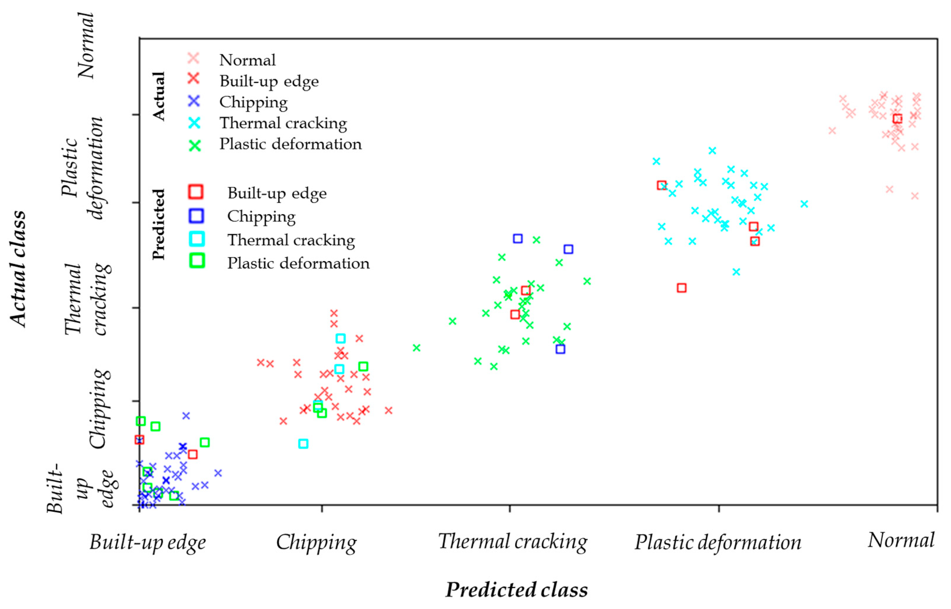
• Built-up edge: Built-up edge is produced due to the adhesion of workpiece material pressure welded to the tooltip as a consequence of sufficient temperature, high pressure, and chemical affinity at the tool–work interface [74]. In due course, the built-up edge breaks down and takes cutting-edge pieces, leading to rapid flank wear and chipping. Built-up edges appear as shiny portions built on the cutting tool’s flank face, leading to cutting-edge chipping and smaller craters or pits on the tool’s rake face [75]. This mode of failure typically occurs while machining stainless steels, superalloys, and non-ferrous materials with lower cutting feeds and speeds. Its prevention requires increased feed rate and speed, selection of a sharper insert with a smoother rake face, and application of coolants at an improved concentration [76].
• Chipping: Chipping occurs due to two main reasons; one is in-built cracks within the material, and the other is the unstable mechanical behavior of the material. Additionally, excessive machining vibrations also lead to cutting-edge chipping. Moreover, rigid inclusions on the surface of the work and intermittent cutting results in localized stress concentrations forming cracks and, ultimately, causing chipping [77]. The appearance of chipping is smaller bits generated due to the breaking of the cutting edge. Machining of hardening work material usually leads to cutting-edge chipping because of abrasion. Its prevention requires controlled tool–workpiece interaction, minimized deflection, and the use of tough carbide grades. Also, reduced feed and higher cutting speed prevent chipping, particularly at cutter entry or exit [78].
• Thermal cracks: Thermal cracks mainly happen due to excessive thermal loadings affected by higher temperatures at the tool–workpiece interface) or changing temperature gradients. Due to these reasons, stress cracks develop approximately perpendicular to the tool edge, ultimately pulling out carbide pieces from the edge to the chip produced [79]. Thermal cracks are primarily witnessed in interrupted turning and milling. This also affects the cooling of tools and workpieces due to the intermittent flow of coolant, leading to thermal cracks. Its prevention requires the application of uninterrupted coolant flow, selecting tough carbide grades, reducing feed and speed, and using a tool with free-cutting geometry to reduce heat [80].
• Plastic deformation: A thermally overloaded tool–workpiece interface leads to plastic deformation. Extreme heating makes the work material soften and is followed by mechanical overloads; the pressure acting on the cutting edge deforms the tooltip and finally breaks down, or rapid flank wear occurs [81]. A deformed cutting edge is the typical appearance of plastic deformation in a tool. One should be cautious when differentiating plastic deformation from flank wear as they resemble one another. Due to their high strength, machining superalloys, strain-hardened surfaces, or hard steels cause plastic deformation. The main reason behind this is the generation of higher cutting temperatures due to high cutting speeds and feeds. Its prevention requires the application of uninterrupted coolant, reduced cutting speeds and feeds, use of a large nose radius, and choosing a wear-resistant and harder carbide grade [82].

3. Experimentation for Signal Acquisition

The signal acquisition process was undertaken in the industrial environment of TAN ENGINEERS Ltd., Pune. The arrangement was set for performing face-milling operations that consisted of a Machining Center, Mild Steel cuboid in the proportion of ${ 8}^{″}\times 6^{″}\times {0.5}^{″}$, HSS milling cutter of four carbide-coated flutes, accelerometer, and data acquisition system as shown in Figure 4. This acquired signal corresponds to the vibration signatures generated due to healthy and faulty tools during the machining process. Researchers commonly employ vibration signals to gain valuable insights into the machining process, as these vibrations are inherent to any machining operation. The operation utilized a spindle speed of $800 \mathrm{r}\mathrm{p}\mathrm{m}$, a feed rate of $500 \mathrm{m}\mathrm{m}/\mathrm{m}\mathrm{i}\mathrm{n}$, and a depth of cut of $0.25 \mathrm{m}\mathrm{m}$. Sensor selection is crucial in collecting authenticated data on which the complete machining learning model is built. Thus, a MEMS-built accelerometer $ADXL335 \left(ATmega2560\right)$ was employed. ADXL335 is a compact and low-power accelerometer. It changes its output by $330 \mathrm{m}\mathrm{i}\mathrm{l}\mathrm{l}\mathrm{i}\mathrm{v}\mathrm{o}\mathrm{l}\mathrm{t}\mathrm{s}$ per input acceleration of $9.81 {\mathrm{m}/\mathrm{s}}^2$ yielding a sensitivity of $330 \mathrm{m}\mathrm{i}\mathrm{l}\mathrm{l}\mathrm{i}\mathrm{v}\mathrm{o}\mathrm{l}\mathrm{t}\mathrm{s}/\mathrm{g}$. The acceleration can be measured in the range of $\pm 3 \mathrm{g}$. Moreover, it offers specific bandwidth selection by three capacitors ($C_X, C_Y, C_Z$) at the $X-out, Y-out, Z-out$ channels, making it appropriate and reliable for use cases within a frequency span of $0.5 \mathrm{H}\mathrm{z} \mathrm{to} 1600 \mathrm{H}\mathrm{z}$ for the $X \mathrm{a}\mathrm{n}\mathrm{d} Y axes$, and $0.5 \mathrm{H}\mathrm{z} \mathrm{to} 550 \mathrm{H}\mathrm{z}$ for the $Z-axis$. Therefore, the signal can be filtered to the desired bandwidth by selecting appropriate capacitors. A suitable microcontroller was utilized for data processing, which provides 16 analog ports for reading the analog data from the accelerometer and converting it into digital format for further processing. The programming was carried out using the Integrated Development Environment.

The sampling frequency was set at 500 Hz in this research, which is considerably higher than the minimum sampling frequency according to the Nyquist criterion. The acquired data were recorded column-wise into Microsoft Excel for seamless analysis. The pilot study was conducted with the inclusion of signals pertaining to all three directions. However, the findings of this study demonstrate that the signal in the Z direction exhibits a higher degree of sensitivity toward the faults that were investigated. Therefore, we consciously opted to focus on the Z direction for signal analysis, as it corresponds to the vertical orientation along the axis of the milling cutter. The vertical rotation of the milling cutter holds profound significance in monitoring the tool’s axial vibrations. Axial vibrations are indicative of cutting forces leading to tool faults. The analysis of the Z-direction signal facilitated the identification of abnormal tool behavior, including occurrences of abnormal tool behavior of built-up edges, chipping, plastic deformation, tool breakage, etc. The cutter in this experiment utilized four carbide-coated flutes and five tool configurations/labels. The first label, designated as “A”, introduced all-new flutes making it a healthy configuration. In addition, label “B” consisted of the three all-new flutes, the same as label “A”, while the flute with a built-up edge was placed at the last position. Similarly, label “C” involved a flute with chipping in the fourth place, “D” involved a flute with thermal cracking, and “E” involved a flute with plastic deformation. These distinctive tool labels offer a range of typical vibration signatures for training and testing the accuracy of the classifiers while also enabling a comprehensive comparison of the results.

4. Signal Representation and Transformation

Vibration signals are primarily captured using accelerometers, and describe their variation with respect to time; therefore, the signal is called a time-domain signal. They narrate the trend of mechanical oscillations or vibrations of an object or system as shown in Figure 5. Most commonly, their application is found in the domains of fault diagnosis—condition monitoring of structures or machine elements. Transforming vibration signals from the time domain to frequency domains using Fourier transform (FT) is a standard practice of signal processing that enables the analysis of distinct frequency components in a signal corresponding to faults or abnormalities in structures or machine elements. FT decomposes the signal into a summation of sine and cosine waves at different frequencies allowing the recognition of dominating frequencies accountable for specific mechanical faults, such as imbalance or resonance, assisting condition monitoring for fault diagnosis. Figure 5 shows the time-domain vibration signal corresponding to various tool conditions. The signal can also be transformed into a time–frequency domain to analyze the dynamic behavior of vibration signals signified by transient events or non-stationary behavior. Time–frequency transformation describes the change in the frequency content of a signal over time, assisting in the discovery of time-varying or intermittent defects. Wavelet transformation deals with localized time–frequency analysis, providing frequency evidence as well as transient event timing. Therefore, it becomes suitable to catch the temporal variations of a signal or identify transient failures. Wavelet analysis offers a high time resolution in interest regions.

The entire signal (from the tool’s entry into the workpiece to its exit) obtained from the sensor was utilized for calculating measures. The entire signal from start to finish was analyzed to capture the complete vibration behavior of the cutting tool during the entire machining process. This approach assists the capability of machine learning algorithms to recognize the dynamic variations in the tool’s condition throughout its usage. Once the primary transformation is undertaken while analyzing vibration signals, some statistical tools are used to quantify the faulty events. One such tool is histograms, which provide insights into quantifying signal characteristics and distribution as shown in Figure 6. A few signal characteristics and distributions exhibited by histograms are discussed.

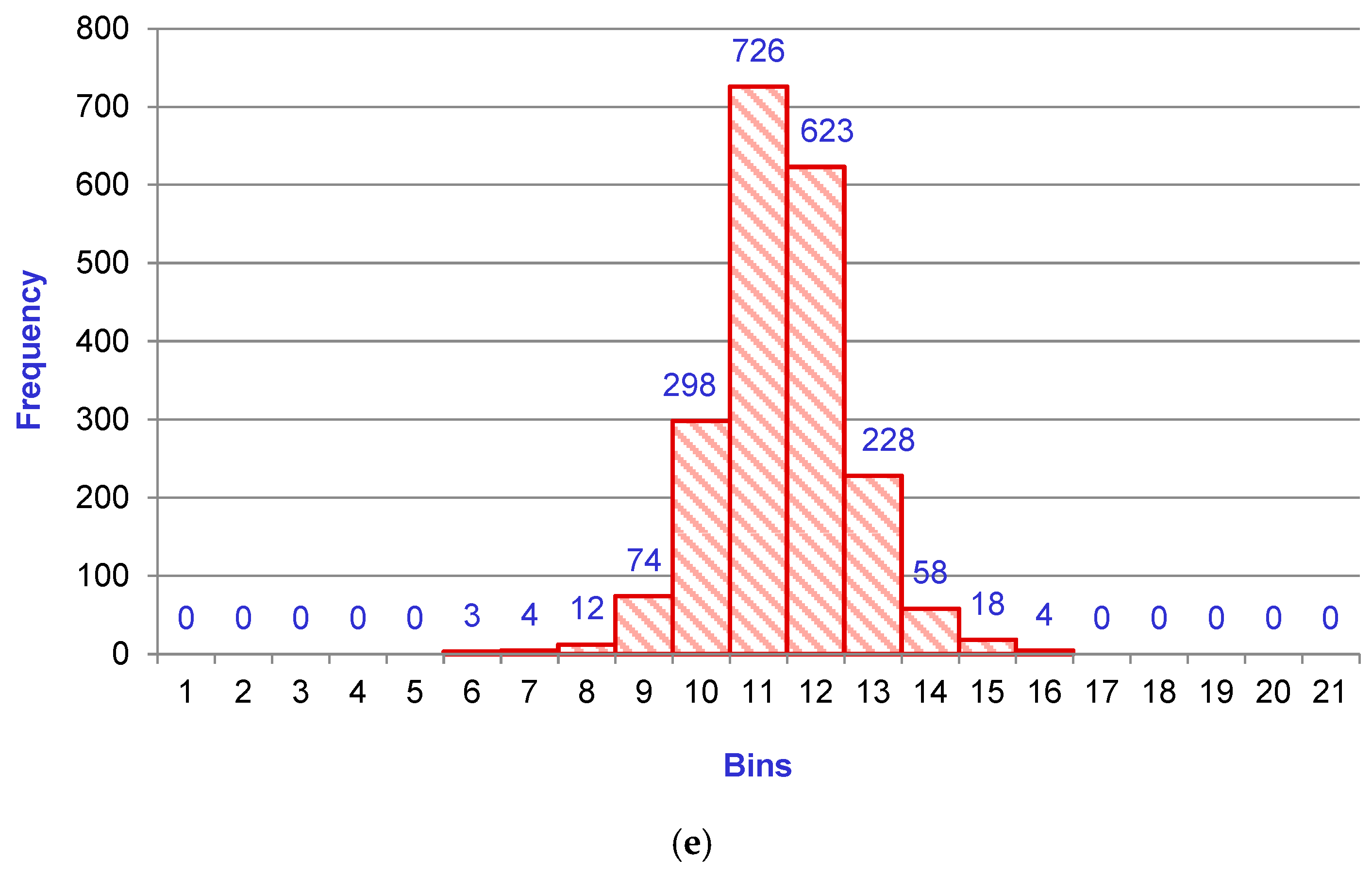
• Amplitude Distribution: A histogram built of vibration signals provides evidence of the amplitude distribution within the collected signal to exhibit its spread and range.
• Peak Values: The histogram highlights the peak frequency and its incidence corresponding to certain abnormalities or events in structures or machine elements being monitored.
• Statistical Parameters: Histograms also assist in the calculation of statistical features of the vibration signal, such as skewness, kurtosis, and standard deviation, to judge the variability, shape, and central tendency of the vibration signal distribution.
• Energy Distribution: Histograms built based on the energy contained inside specific frequency bands allow the analysis of the vibration signals’ frequency-dependent features.
• Signal Characteristics: Histograms also reveal modes or patterns of vibration. For instance, clusters or multi-peaks in a typical histogram designate the existence of different vibration components or modes.
• Trends and Changes: Rapid deviations or shifts in the normal histogram distribution indicate wear, faults, or other changes in structures or machine elements.

Plotting histograms of vibration signals is employed for various reasons, for example, to classify abnormal patterns, discover anomalies or faults, assess the health of structures or machine elements, and provide insights for predictive maintenance strategies. The selection of appropriate histogram smoothing and binning techniques needs careful consideration based on the particular vibration characteristics.

5. Feature Engineering

A widespread feature engineering method for vibration signals is extracting statistical measures such as mean, standard deviation, skewness, and kurtosis to understand the signal’s central tendency, variability, shape, etc. Histogram features are one such statistical representation of data in a graphical form. The dataset is divided into discrete bins or intervals to count the number of data points within each bin. Some standard histogram features include:

• Bin counts: Bin counts specify that the number of observations falls within every bin of the histogram indicating the frequency of specific incidence.
• Bin heights: Bin height specifies the altitude of every bin of the histogram representing the graphic view of the distribution’s shape through the relative frequency of observations within a particular bin.
• Bin widths: Bin widths specify the thickness of every bin of the histogram determining the range of observations considered by every bin which affects the granularity or smoothness of the distribution.
• Bin centers: Bin centers specify the central value or midpoint of every bin.
• Skewness: Skewness specifies the histogram’s asymmetry indicating whether the observations are skewed to the right or left from its mean value.
• Kurtosis: Kurtosis specifies a histogram’s flatness or peakedness quantifying deviation from a normal distribution.
• Mean: To judge the central tendency, the average value of the observations plays an important role.
• Standard Deviation: Standard deviation measures the spread or dispersion of the observations around their average value indicating the variability of the distribution.

The procedure used for plotting histograms is stated here.

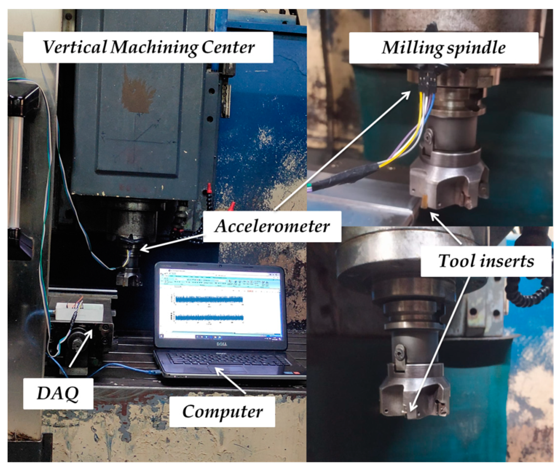
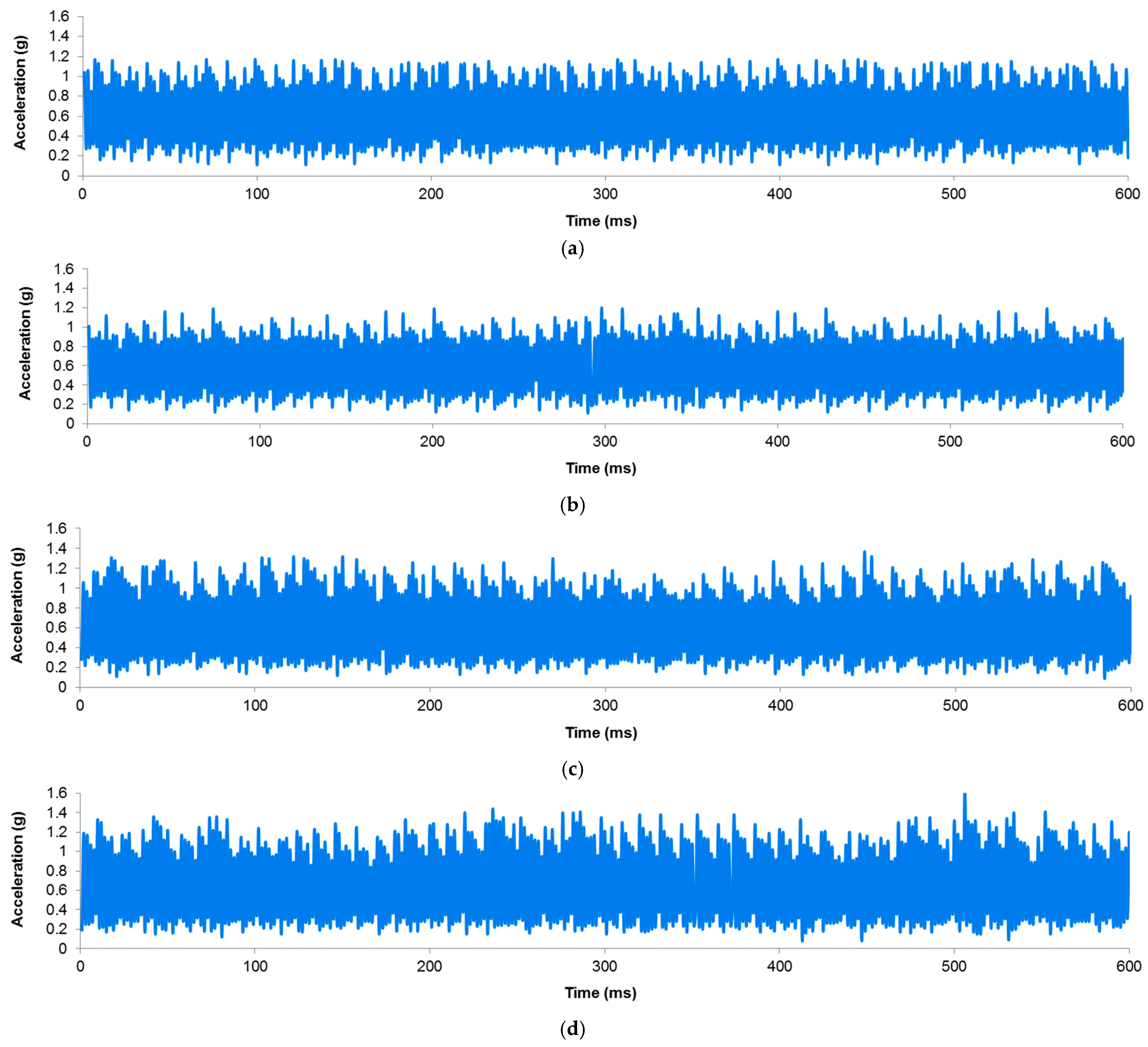
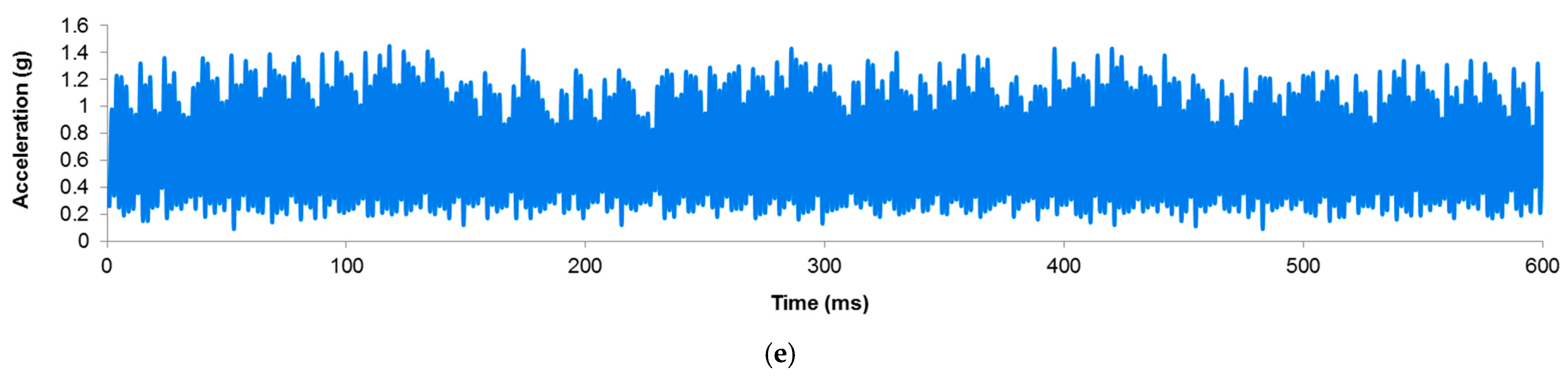
• Signal acquisition: During the face-milling operation, vibration data were collected using the accelerometer, which was located near the milling cutter spindle holder. The accelerometer measures the vibration in terms of acceleration experienced by the milling cutter for various tool conditions. The data were acquired continuously throughout the face-milling operation, considering the vibrations in the Z direction.
• Signal pre-processing: Before constructing histograms, the raw vibration signals were pre-processed using filters to remove noise or irrelevant information.
• Creation of bins: The vibration data were divided into smaller intervals or bins. Each bin signifies a specific range of acceleration. The number of bins and range for each bin were selected based on the data dynamics.
• Counting Observations: The number of acceleration observations that fell within that specific range was counted for each bin. The count represents the frequency of observations within each bin, reflecting how often the acceleration values occur in that range.
• Visualization: Finally, histograms were plotted where the X-axis shows the bins or ranges of acceleration values, and the Y-axis shows the corresponding frequency or count of observations in each bin.

Figure 7 shows the histogram distribution of time-domain vibration signals corresponding to various tool conditions. These features are generally employed in various domains such as pattern recognition, data analysis, computer vision, and image processing, to name a few. Valuable insights into the patterns and features of histograms can be analyzed for better analysis and understanding of the dataset.

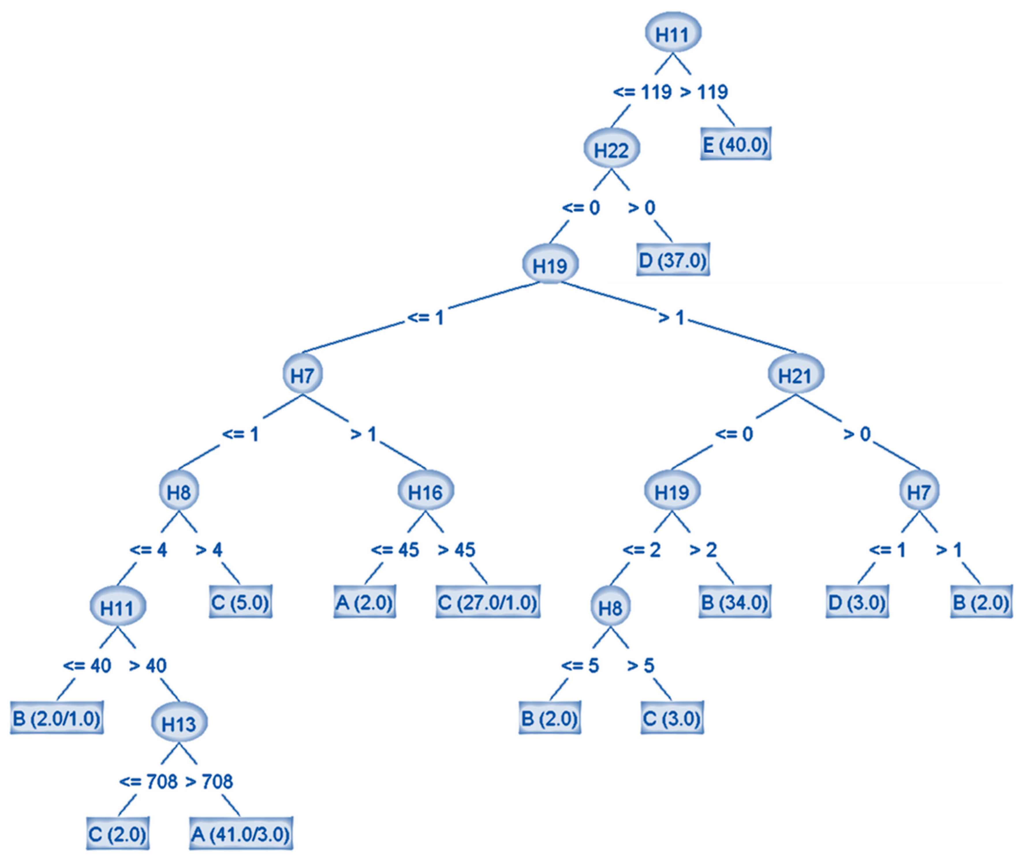
6. Design of Partial C4.5 Decision Tree

Partial C4.5 (PART), also known as C4.5 Rule Induction, extends the C4.5 decision tree, first introduced by Ross Quinlan [83]. It aims at building a set of classification/regression rules. The C4.5 decision tree initiates its construction by recursively splitting attributes and features. However, the C4.5 tree often becomes excessively complex and likely to overfit, mainly while dealing with high-dimensional or noisy instances. PART introduced a rubric-based method to address these issues instead of constructing a wide-ranging decision tree [84]. It builds rubrics consisting of conditions based on thresholds of features and corresponding conditions to be classified. They are produced with the consideration of the most frequent features-class combination within each data split [85]. PART provides an improved interpretation of decisions taken using rubrics, and produces compact models by avoiding overfitting with additional splits [86].

The PART algorithm works as follows.

• Initialization of the rule set as empty.
• For each data split:
  • Construct a rubric with the same class if the split is pure, indicating zero entropy (covers observations of only a single label).
  • If the split is impure, indicating entropy more than zero (covers observations of multiple labels), choose the most frequent features-class combination and construct a rubric with the same features-class combination.
  • Again, if the split of step “b” is not pure, choose the best attribute according to Gini or information gain criteria.
  • Divide the split according to attribute value and make new splits for every value.
  • Recurse on every new split until termination is fulfilled.
• Once all partitions have been processed, the algorithm outputs the rules.

The PART appears flexible in handling noisy observations by not strictly testing purity at every split, similar to C4.5. Induction of PART avoids unnecessary branch creation if branches do not contribute considerably to performance [87]. Therefore, it becomes a comprehensible and simpler model than traditional decision trees. PART is principally beneficial where interpretability is vital, such as in legal decision-making or medical diagnosis [88]. However, it sometimes communicates differently over C4.5, mainly with high or complex correlated observations. Hence, the selection between PART and C4.5 is contingent on the characteristics of the problem and specific requirements. In several ways, PART differs from other tree family classifiers, as stated here.

• Random Forest (RF): The principle of random forest is an ensemble that constructs multiple decision trees and averages out their predictions. Multiple trees are built using training instances, and their feature subset is selected randomly. Oppositely, PART uses a single set of rubrics by recursive splitting attribute values of the data. RF aims to improve generalization and reduce variance by averaging predictions of multiple random trees, while PART emphasizes generating interpretable rubrics.
• Logistic Model Trees (LMT): The logistic regression is combined with decision trees to design LMTs. The induction of LMT is similar to conventional decision trees; however, while taking decisions at leaf nodes, it estimates class probabilities using logistic regression. LMT captures linear associations between attributes and corresponding labels. On the other hand, PART exhibits rubrics considering attributes and majority labels of every split without explicitly modeling logistic regression.
• Random Tree (RT): Random Tree is another variant of a decision tree that chooses attributes randomly at every partition point using a single tree in place of an ensemble-like random forest. Random Tree handles high-dimensional datasets and helps to reduce overfitting. However, unlike PART, it does not produce rubrics explicitly.
• Hoeffding Tree (HT): Hoeffding Tree handles datasets containing larger instances. A Hoeffding bound decides judgment about the tree structure, avoiding re-processing the complete dataset. They are incremental and adapt to concept drift. In contrast, PART does not address concept drift or streaming situations.
• Rotation Forest with Enhanced Performance Trees (REPT): REPT is an extension of Rotation Forest, an ensemble method based on extracting features using principal component analysis. REPT further augments the performance of the Rotation Forest with the help of Enhanced Performance Trees (EPTs) by splitting attributes through information gain. REPT efficiently trains complex associates between attributes and handles data with higher dimensions. PART, instead, aimed at creating a concise set of rubrics for interpretability instead of engaging feature extraction or ensemble methods.

Different tree family classifiers have their own strengths and weaknesses. Some applications must focus on challenges like high dimensionality, streaming data, or improving predictive performance. However, PART explicitly emphasizes generating concise models and rubric-based interpretability owing to ambiguity in vibration signatures between tool faults. Therefore, the PART classifier has been a choice for current research, given its interpretability, predictive accuracy, scalability, or adaptability to changing characteristics of tool spindle vibrations.

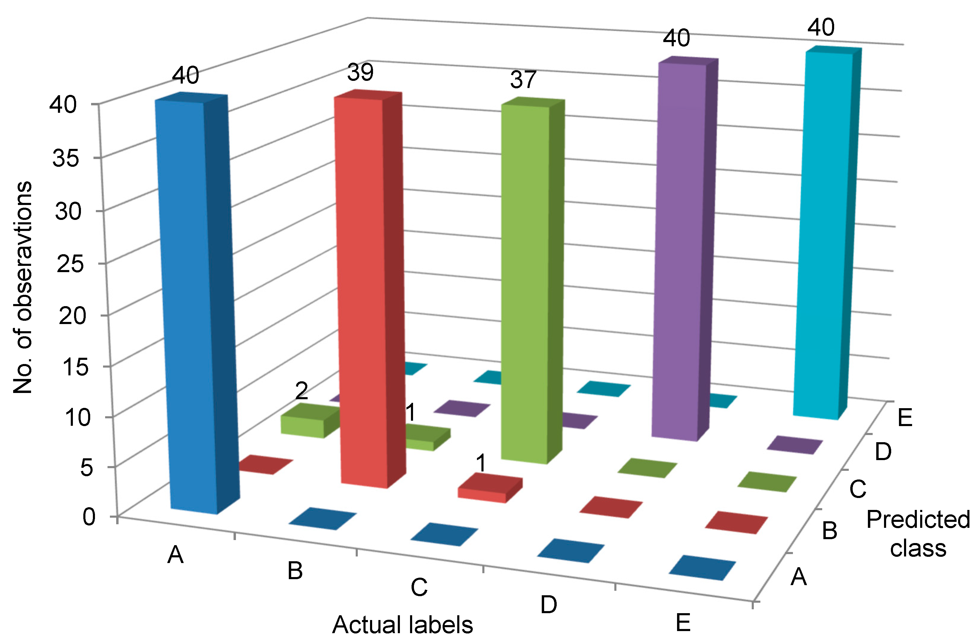
7. Results and Discussion

This section provides findings and outcomes trained model of PART and its interpretation using performance indicators evaluation measures and statistical metrics. First, the PART model is trained and tested through a ten-fold cross-validation method—a commonly used technique to assess model performance and generalization.

The dataset is split into ten folds, called subsets, where every fold has a chance to be trained and tested iteratively. For ensuring a robust assessment of PART’s performance and estimating its generalization capability, cross-validation is extensively considered in ML to mitigate the overfitting issues and provide more reliable performance estimation. The tree developed by this technique is shown in Figure 8. The binary tree with various branching test conditions at 11 branch nodes consisted of 13 leaves denoting decisions taken for classification and one root node, making a total size of 25. The tree initiates its training at a root node that evaluates if the H11 attribute is not more than or equivalent to feature value 119. If true, it continues to be trained via the branch on the left side, or if false, it decides the branch on the right side as all 40 observations of normal condition, i.e., label “F” is correctly classified. The decision structure shows a bunch of decision rubrics made by testing different attributes (such as H11, H22, H19, H7, H8, H13, H16, and H21) and corresponding thresholds. These decision rubrics decide the pathway to take through the tree up to a leaf node is reached to provide the predicted label for a particular input vibration signal. Therefore, all 13 leaf nodes represent a predicted label (A—Built-up edge; B—Chipping; C—Thermal cracking; D—Plastic deformation; or F—normal tool) along with the number of observations. For instance, if the pathway directs to a leaf node “B”—Chipping, it designates that the classifier predicts the vibration signal belonging to label “B”—Chipping, and the observations agreeing to it are stated in brackets. Among all 21 attributes, only 8 attributes (such as H11, H22, H19, H7, H8, H13, H16, and H21) are considered by decision trees, as these attributes show dissimilarity between the five tool conditions. The attributes the decision tree discarded while training shows the similarity between classes. Thus, the process is regarded as attribute selection. With eight attributes (such as H11, H22, H19, H7, H8, H13, H16, and H21) chosen by the decision tree, the PART classifier is trained, and results are discussed.

The confusion matrix denotes the performance of a PART classifier that predicted five different labels of tool condition: A—Built-up edge, B—Chipping, C—Thermal cracking, D—Plastic deformation, or F—normal tool. The rows correspond to the actual labels, while the columns correspond to the predicted labels. Here is an interpretation of the confusion matrix.

• Label A, i.e., built-up edge (actual) was correctly classified as A (predicted) 40 times and there is no misclassification.
• Label B, i.e., chipping (actual) was correctly classified as B (predicted) 39 times and misclassified as C once.
• Label C, i.e., thermal cracking (actual) was correctly classified as C (predicted) 37 times and misclassified as A twice and B once.
• Label D, i.e., plastic deformation (actual) was correctly classified as D (predicted) 40 times and there is no misclassification.
• Label F, i.e., normal (actual) was correctly classified as F (predicted) 40 times and there is no misclassification.

From the matrix shown in Figure 9, it can be observed that the model achieved perfect accuracy on the given dataset, since the 196 diagonal elements represent the correct predictions of 98%. These misclassifications imply that the model had some difficulty distinguishing between Label B and Label C. It is worth noting that the model did not misclassify any instances as Label A or Label D or Label F, which suggests that these classes were well-separated and easily distinguishable by the model. Overall, the misclassifications are relatively minimal, i.e., only four observations, demonstrating a robust performance by the model. A Kappa value of 0.975 suggests a very high level of agreement between the model’s predictions and the true classes. A mean absolute error of 0.0148 indicates that, on average, the model’s predictions were off by approximately 0.0148 units. The root mean squared error of 0.0861 indicates the average magnitude of the model’s prediction errors. A relative absolute error of 4.631% indicates that, on average, the model’s predictions deviate by approximately 4.631% from the mean of the actual values. A relative absolute error of 21.5196% indicates the average magnitude of the prediction errors relative to the range of the actual values. The detailed performance of the PART classifier on the training dataset is discussed and shown in

Table 3. PART classifier performance evaluation using training dataset.

Performance Matrices
Matrices					Value	Percentage
Correctly Classified Instances					196	98%
Incorrectly Classified Instances					4	2%
Kappa statistic					0.975	-
Mean absolute error					0.0148	-
Root mean squared error					0.0861	-
Relative absolute error					-	4.631%
Root relative squared error					-	21.5196%
Detailed performance
Class	A	B	C	D	F	Weighted Avg.
TP Rate	1.000	0.975	0.925	1.000	1.000	0.980
FP Rate	0.013	0.006	0.006	0.000	0.000	0.005
Precision	0.952	0.975	0.974	1.000	1.000	0.980
Recall	1.000	0.975	0.925	1.000	1.000	0.980
F-Measure	0.976	0.975	0.949	1.000	1.000	0.980
MCC	0.970	0.969	0.937	1.000	1.000	0.975
ROC Area	0.994	0.997	0.989	1.000	1.000	0.996
PRC Area	0.952	0.986	0.951	1.000	1.000	0.978

. The algorithm attained a True Positive (TP) Rate of 1.000, corresponding to all correctly identified observations of label A. The False Positive (FP) Rate is 0.013, showing a lower misclassification rate of other labels as A. Precision is 0.952, indicating a comparatively lower false positives rate. The Recall is 1.000, suggesting that the algorithm properly recognized all actual observations of label A.

The F-Measure is 0.976, which is the summation of Recall and Precision into a single metric. The Matthews Correlation Coefficient (MCC) is 0.970, which suggests a strong association between actual and predicted labels. The ROC Area is 0.994, showcasing excellence in terms of observations ranking. The PRC Area is 0.952, representing the region prescribed in the Precision–Recall curve. Similarly, matrices for other labels can be examined. To summarize, these metrics show that the algorithm exhibited higher F-Measure, Recall, Precision, and Accuracy for every label, along with an overall weighted average is also higher. Moreover, the PRC, ROC, and MCC Area scores perform robustly distinguishing various labels. Figure 10 shows the confusion matrix for the PART classifier using cross-validation on the training dataset, and

Table 4. PART classifier performance evaluation using cross-validation on the training dataset.

Performance Matrices
Matrices					Value	Percentage
Correctly Classified Instances					173	86.5%
Incorrectly Classified Instances					27	13.5%
Kappa statistic					0.8313	-
Mean absolute error					0.0575	-
Root mean squared error					0.2267	-
Relative absolute error					-	17.958%
Root relative squared error					-	56.6627%
Detailed performance
Class	A	B	C	D	F	Weighted Avg.
TP Rate	0.875	0.800	0.750	0.900	1.000	0.865
FP Rate	0.063	0.038	0.044	0.019	0.006	0.034
Precision	0.778	0.842	0.811	0.923	0.976	0.866
Recall	0.875	0.800	0.750	0.900	1.000	0.865
F-Measure	0.824	0.821	0.779	0.911	0.988	0.864
MCC	0.778	0.777	0.728	0.890	0.985	0.832
ROC Area	0.941	0.907	0.895	0.953	0.997	0.938
PRC Area	0.748	0.779	0.753	0.894	0.976	0.830

states its detailed performance.

Several evaluation metrics are discussed to compare the performance of the PART classifier in the three cases (i.e., training dataset, cross-validation, and test data). In terms of correctly classified instances, the classifier performed best on the training dataset, i.e., 98% (196 out of 200 instances), followed by the ten-fold cross-validation on the training dataset, i.e., 80% (48 out of 60 instances) and the test data, i.e., 86.5% (173 out of 200 instances). The kappa statistic is highest for the training dataset, i.e., 0.975, followed by the ten-fold cross-validation on the training dataset, i.e., 0.8313 and 0.7489 on the test data. The training dataset has the lowest MAE, i.e., 0.0148, followed by the ten-fold cross-validation on the training dataset, i.e., 0.0575 and 0.088 on the test data. Like the MAE, the training dataset has the lowest RMSE, i.e., 0.0861, followed by the ten-fold cross-validation on the training dataset, i.e., 0.2267 and 0.2805 on the test data. Figure 11 shows the confusion matrix for the PART classifier using the test dataset and

Table 5. PART classifier performance evaluation using the test dataset.

Performance Matrices
Matrices					Value	Percentage
Correctly Classified Instances					48	80%
Incorrectly Classified Instances					12	20%
Kappa statistic					0.7489	-
Mean absolute error					0.088	-
Root mean squared error					0.2805	-
Relative absolute error					-	27.4118%
Root relative squared error					-	69.8654%
Detailed performance
Class	A	B	C	D	F	Weighted Avg.
TP Rate	0.867	0.571	0.900	0.700	1.000	0.800
FP Rate	0.044	0.065	0.040	0.040	0.061	0.051
Precision	0.867	0.727	0.818	0.778	0.786	0.796
Recall	0.867	0.571	0.900	0.700	1.000	0.800
F-Measure	0.867	0.640	0.857	0.737	0.880	0.793
MCC	0.822	0.553	0.828	0.689	0.859	0.745
ROC Area	0.911	0.702	0.964	0.830	0.969	0.868
PRC Area	0.784	0.516	0.775	0.594	0.786	0.689

states its detailed performance.

Overall, the PART classifier performs better on the training dataset than the cross-validation. This is anticipated, as the classifier was educated on the training data and was overfitted. Figure 12 shows PART classifier performance errors in pictorial form. The k-fold cross-validation usually has a lower performance to some extent than the training data, and the evaluation of the model using independent test data has the lowermost performance among the three circumstances.

8. Conclusions

The current investigation focused on employing an ML-based health-monitoring framework for detecting and analyzing damage types arising in cutting tools during face milling. The PART algorithm was trained to classify faults (built-up edges, chipping, thermal cracking, and plastic deformation) in terms of histogram features extracted from spindle vibrations as an indicator of tool conditions and was found appropriate.

• The decision tree construction comprised 11 branches, 13 leaves, and a total size of 25. Eight features were chosen while training the tree, as there was a difference between the four faulty and normal tool labels, while the rejected ones showed similarity.
• The PART algorithm attained a desired accuracy of 98% when learning the rubrics on training data. It truly categorized labels A—Built-up edge, D—Plastic deformation, and F—normal tool without a single misclassification. However, the algorithm faced confusion segregating labels B—Chipping and C—Thermal cracking, following some misclassifications. Nonetheless, the overall misclassifications were negligible, signifying a robust model.
• The evaluation metrics further demonstrate the usefulness of the PART algorithm. A Kappa value showed higher agreement between the actual labels and corresponding predictions. The mean absolute and root mean squared error denoted the average prediction errors. The relative absolute and relative squared errors showed insights into the deviance between the actual labels and corresponding predictions.
• Detailed evaluation of the PART algorithm on the training data exhibited higher true positives, Matthews Correlation Coefficient, Recall, F-Measure, Precision, ROC Area, and PRC Area. These metrics specified correct identification and distinction of various tool conditions.
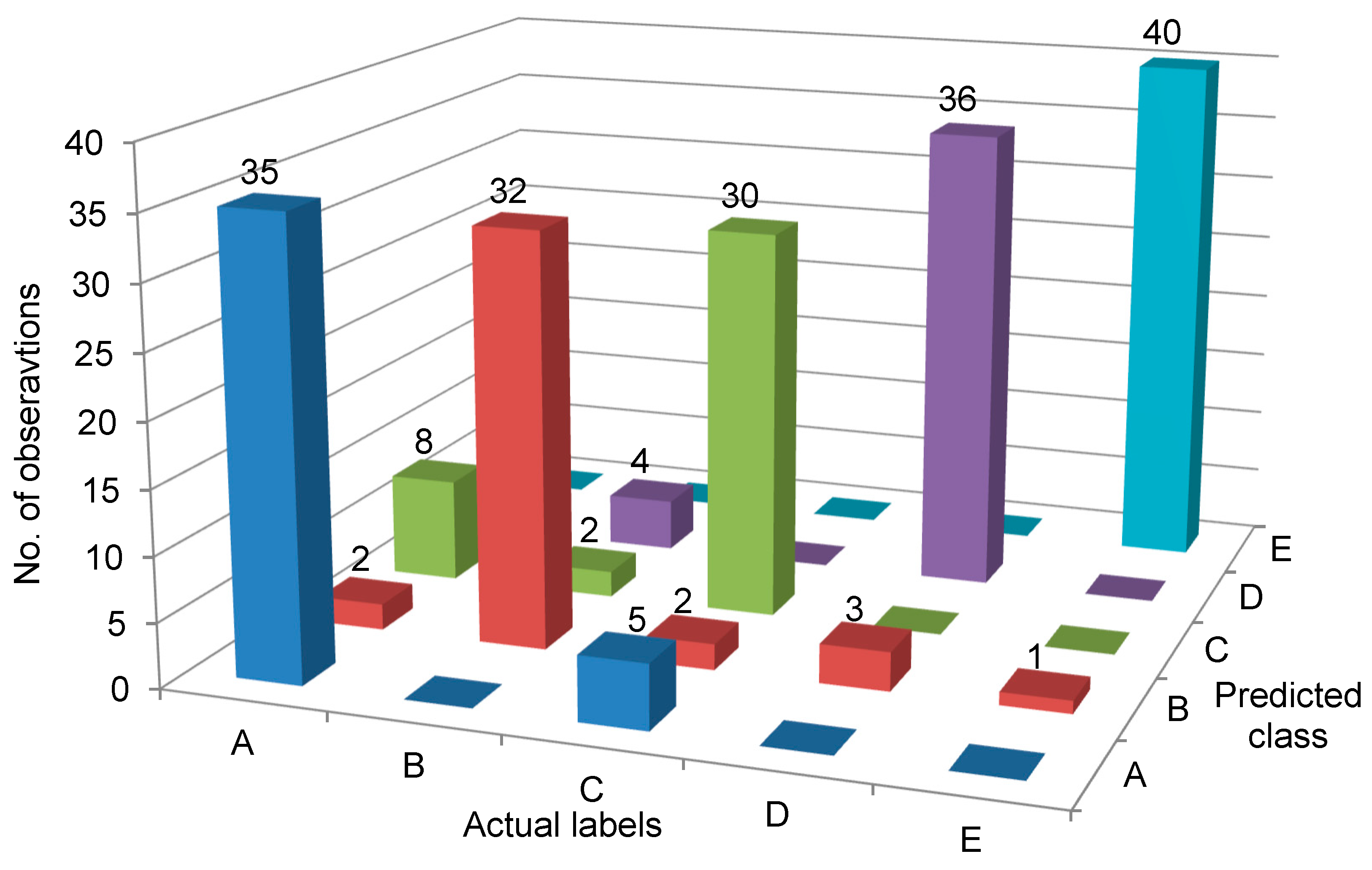
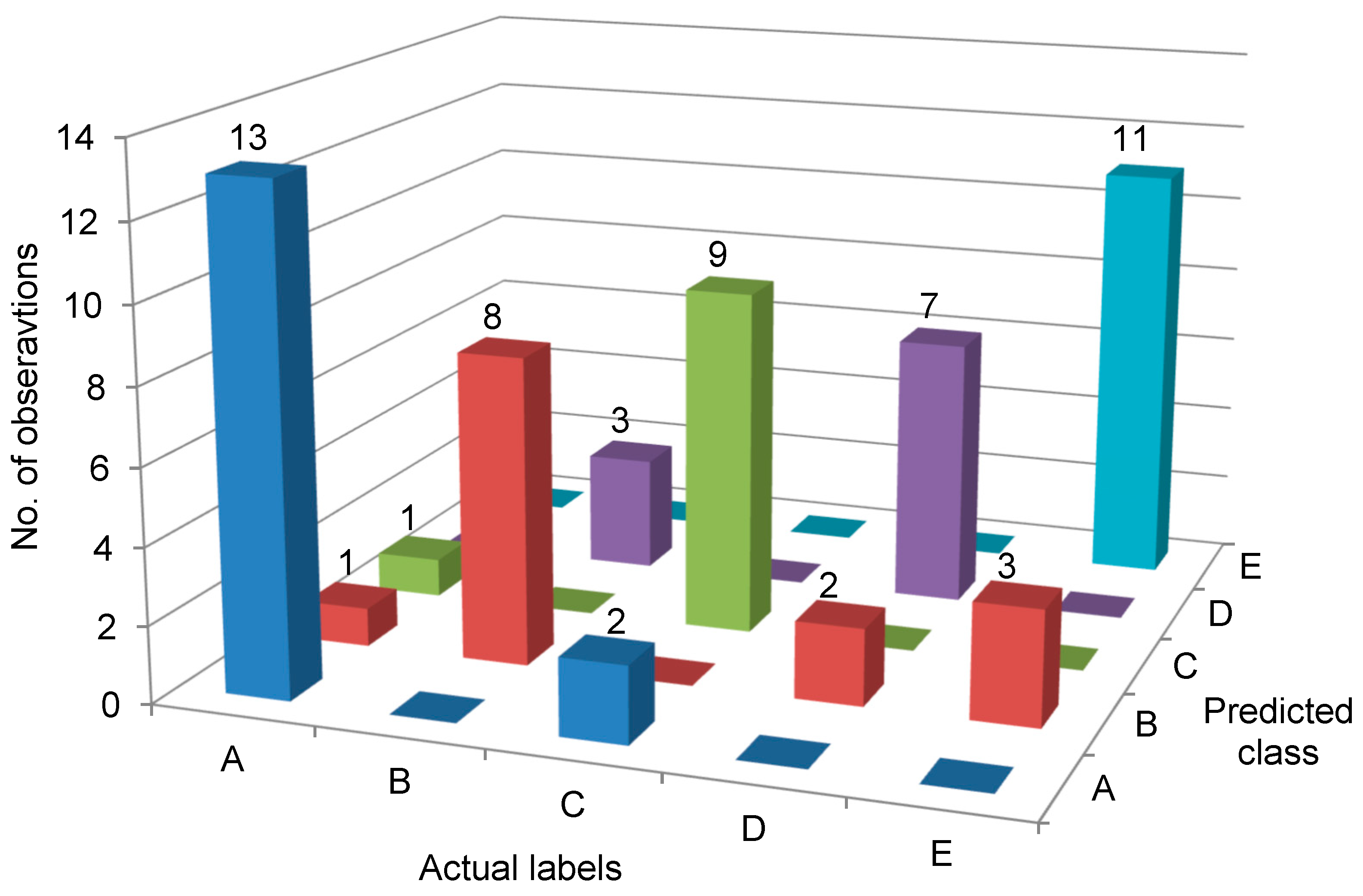
• The robustness of the PART classifier was compared in three scenarios; it executed best on the training data, followed by the k-folds cross-validation and the test data. The assessment metrics exhibited lower error and higher accuracy in all three scenarios, eliminating the potential concern of overfitting.
• In conclusion, the method demonstrated herein appears to be robust for categorizing tool labels based on the histogram features of the vibration dataset. However, it is vital to be careful while applying the model to unlabeled data, as the performance may differ from trained rubrics. The study highlighted the significance of vibration analysis and machine learning for condition monitoring, enabling time-to-time maintenance or replacing cutting tools, therefore improving productivity and efficiency.

References

- Smith, S.; Tlusty, J. An Overview of Modeling and Simulation of the Milling Process. J. Eng. Ind. 1991, 113, 169–175. [Google Scholar] [CrossRef]
- Binali, R.; Demirpolat, H.; Kuntoğlu, M.; Sağlam, H. Machinability investigations based on tool wear, surface roughness, cutting temperature, chip morphology and material removal rate during dry and MQL-assisted milling of Nimax mold steel. Lubricants 2023, 11, 101. [Google Scholar] [CrossRef]
- Tlusty, J. Machine Dynamics. In Handbook of High-Speed Machining Technology; Chapman and Hall Advanced Industrial Technology Series; King, R.I., Ed.; Springer: Boston, MA, USA, 1985. [Google Scholar] [CrossRef]
- Morelli, L.; Grossi, N.; Campatelli, G.; Scippa, A. Surface location error prediction in 2.5-axis peripheral milling considering tool dynamic stiffness variation. Precis. Eng. 2022, 76, 95–109. [Google Scholar] [CrossRef]
- Lazkano, X.; Aristimuño, P.X.; Aizpuru, O.; Arrazola, P.J. Roughness maps to determine the optimum process window parameters in face milling. Int. J. Mech. Sci. 2022, 221, 107191. [Google Scholar] [CrossRef]
- Usca, Ü.A.; Uzun, M.; Şap, S.; Kuntoğlu, M.; Giasin, K.; Pimenov, D.Y.; Wojciechowski, S. Tool wear, surface roughness, cutting temperature and chips morphology evaluation of Al/TiN coated carbide cutting tools in milling of Cu–B–CrC based ceramic matrix composites. J. Mater. Res. Technol. 2022, 16, 1243–1259. [Google Scholar] [CrossRef]
- Kuntoğlu, M.; Gupta, M.K.; Aslan, A.; Salur, E.; Garcia-Collado, A. Influence of tool hardness on tool wear, surface roughness and acoustic emissions during turning of AISI 1050. Surf. Topogr. Metrol. Prop. 2022, 10, 015016. [Google Scholar] [CrossRef]
- He, Z.; Shi, T.; Xuan, J. Milling tool wear prediction using multi-sensor feature fusion based on stacked sparse autoencoders. Measurement 2022, 190, 110719. [Google Scholar] [CrossRef]
- Shewale, M.S.; Mulik, S.S.; Deshmukh, S.P.; Patange, A.D.; Zambare, H.B.; Sundare, A.P. Novel machine health monitoring system. In Proceedings of the 2nd International Conference on Data Engineering and Communication Technology: ICDECT 2017; Springer: Singapore, 2019; pp. 461–468. [Google Scholar]
- Dhobale, N.; Mulik, S.; Jegadeeshwaran, R.; Patange, A. Supervision of milling tool inserts using conventional and artificial intelligence approach: A review. Sound Vib. 2021, 55, 87–116. [Google Scholar] [CrossRef]
- Binali, R.; Kuntoğlu, M.; Pimenov, D.Y.; Usca, Ü.A.; Gupta, M.K.; Korkmaz, M.E. Advance monitoring of hole machining operations via intelligent measurement systems: A critical review and future trends. Measurement 2022, 111757. [Google Scholar] [CrossRef]
- Gupta, M.K.; Niesłony, P.; Sarikaya, M.; Korkmaz, M.E.; Kuntoğlu, M.; Krolczyk, G.M.; Jamil, M. Tool wear patterns and their promoting mechanisms in hybrid cooling assisted machining of titanium Ti-3Al-2.5 V/grade 9 alloy. Tribol. Int. 2022, 174, 107773. [Google Scholar] [CrossRef]
- Kuntoglu, M. Machining induced tribological investigations in sustainable milling of Hardox 500 steel: A new approach of measurement science. Measurement 2022, 201, 111715. [Google Scholar] [CrossRef]
- Kuntoğlu, M.; Acar, O.; Gupta, M.K.; Sağlam, H.; Sarikaya, M.; Giasin, K.; Pimenov, D.Y. Parametric optimization for cutting forces and material removal rate in the turning of AISI 5140. Machines 2021, 9, 90. [Google Scholar] [CrossRef]
- Karali, P.; Pal, S.K.; Bhattacharyya, K. fuzzy radial basis function (FRBF) network based tool condition monitoring system using vibration signals. Mach. Sci. Technol. Int. J. 2010, 14, 280–300. [Google Scholar]
- Sugumaran, V.; Ramachandran, K.I. Effect of number of features on classification of roller bearing faults using SVM and PSVM. Expert Syst. Appl. 2011, 38, 4088–4096. [Google Scholar] [CrossRef]
- Elangovan, M.; Ramachandran, K.I.; Sugumaran, V. Studies on Bayes classifier for condition monitoring of single point carbide tipped tool based on statistical and histogram features. Expert Syst. Appl. 2010, 37, 2059–2065. [Google Scholar] [CrossRef]
- Elangovan, M.; Babu, D.S.; Sakthivel, N.R.; Ramachandran, K.I. Evaluation of expert system for condition monitoring of a single point cutting tool using principle component analysis and decision tree algorithm. Expert Syst. Appl. 2011, 38, 4450–4459. [Google Scholar] [CrossRef]
- Krishnakumar, P.; Rameshkumar, K.; Ramachandran, K.I. Tool Wear Condition Prediction Using Vibration Signals in High Speed Machining (HSM) of Titanium (Ti-6Al-4V) Alloy. In Proceedings of the Procedia Computer Science, 2nd International Symposium on Big Data and Cloud Computing; 2015; Volume 50, pp. 270–275. [Google Scholar]
- Fatima, S.; Mohanty, A.R.; Naikan, V.N.A. Multiple Fault Classification Using Support Vector Machine in a Machinery Fault Simulator. Vib. Eng. Technol. Mach. Mech. Mach. Sci. 2015, 23. [Google Scholar]
- Drouillet, C.; Karandikar, J.; Nath, C.; Journeaux, A.C.; El Mansori, M.; Kurfess, T. Tool life predictions in milling using spindle power with the neural network technique. J. Manuf. Process. 2016, 22, 161–168. [Google Scholar] [CrossRef]
- Ross, N.S.; Sheeba, P.T.; Shibi, C.S.; Gupta, M.K.; Korkmaz, M.E.; Sharma, V.S. A novel approach of tool condition monitoring in sustainable machining of Ni alloy with transfer learning models. J. Intell. Manuf. 2023, 1–19. [Google Scholar] [CrossRef]
- Laghari, R.A.; Mekid, S. Comprehensive Approach Toward IIoT Based Condition Monitoring of Machining Processes. Measurement 2023, 217, 113004. [Google Scholar] [CrossRef]
- Ahmed, M.; Kamal, K.; Ratlamwala TA, H.; Hussain, G.; Alqahtani, M.; Alkahtani, M.; Alzabidi, A. Tool Health Monitoring of a Milling Process Using Acoustic Emissions and a ResNet Deep Learning Model. Sensors 2023, 23, 3084. [Google Scholar] [CrossRef]
- Natarajan, S.; Thangamuthu, M.; Gnanasekaran, S.; Rakkiyannan, J. Digital Twin-Driven Tool Condition Monitoring for the Milling Process. Sensors 2023, 23, 5431. [Google Scholar] [CrossRef]
- Mohanraj, T.; Uddin, M.; Thangarasu, S.K. Review on sensor design for cutting force measurement. Proc. Inst. Mech. Eng. Part E J. Process Mech. Eng. 2023, 237, 455–466. [Google Scholar] [CrossRef]
- Ou, J.; Li, H.; Huang, G.; Zhou, Q. A Novel Order Analysis and Stacked Sparse Auto-Encoder Feature Learning Method for Milling Tool Wear Condition Monitoring. Sensors 2020, 20, 2878. [Google Scholar] [CrossRef]
- Mohanraj, T.; Jayanthi, Y.; Krishnan, H.; Nithin Aravind, R.S.; Yameni, R. Development of tool condition monitoring system in end milling process using wavelet features and Hoelder’s exponent with machine learning algorithms. Measurement 2021, 173, 108671. [Google Scholar] [CrossRef]
- Yao, Z.; Luo, M.; Mei, J.; Zhang, D. Position dependent vibration evaluation in milling of thin-walled part based on single-point monitoring. Measurement 2021, 171, 108810. [Google Scholar] [CrossRef]
- Shrivastava, Y.; Singh, B. Tool chatter prediction based on empirical mode decomposition and response surface methodology. Measurement 2021, 173, 108585. [Google Scholar] [CrossRef]
- Kuntoğlu, M.; Sağlam, H. Investigation of signal behaviors for sensor fusion with tool condition monitoring system in turning. Measurement 2021, 173, 108582. [Google Scholar] [CrossRef]
- Xu, X.; Wang, J.; Zhong, B.; Ming, W.; Chen, M. Deep learning-based tool wear prediction and its application for machining process using multi-scale feature fusion and channel attention mechanism. Measurement 2021, 177, 109254. [Google Scholar] [CrossRef]
- Finkeldey, F.; Saadallah, A.; Wiederkehr, P.; Morik, K. Real-time prediction of process forces in milling operations using synchronized data fusion of simulation and sensor data. Eng. Appl. Artif. Intell. 2020, 94, 103753. [Google Scholar] [CrossRef]
- Bobyr, M.V.; Yakushev, A.S.; Dorodnykh, A.A. Fuzzy devices for cooling the cutting tool of the CNC machine implemented on FPGA. Measurement 2020, 152, 107378. [Google Scholar] [CrossRef]
- Postel, M.; Bugdayci, B.; Wegener, K. Ensemble transfer learning for refining stability predictions in milling using experimental stability states. Int. J. Adv. Manuf. Technol. 2020, 107, 4123–4139. [Google Scholar] [CrossRef]
- Hesser, D.F.; Markert, B. Tool wear monitoring of a retrofitted CNC milling machine using artificial neural networks. Manuf. Lett. 2019, 19, 1–4. [Google Scholar] [CrossRef]
- Herwan, J.; Kano, S.; Ryabov, O.; Sawada, H.; Kasashima, N.; Misaka, T. Retrofitting old CNC turning with an accelerometer at a remote location towards Industry 4.0. Manuf. Lett. 2019, 21, 56–59. [Google Scholar] [CrossRef]
- Cuka, B.; Kim, D. Fuzzy logic based tool condition monitoring for end-milling. Robot. Comput. -Integr. Manuf. 2017, 47, 22–36. [Google Scholar] [CrossRef]
- Harris, K.; Triantafyllopoulos, K.; Stillman, E.; Mcleay, T. A multivariate control chart for autocorrelated tool wear processes. Qual. Reliab. Eng. Int. 2016, 32, 2093–2106. [Google Scholar] [CrossRef] [Green Version]
- Sevilla, P.; Robles, J.; Jauregui, J.; Jimenez, D. FPGA-based reconfigurable system for tool condition monitoring in high-speed machining process. Measurement 2015, 64, 81–88. [Google Scholar] [CrossRef]
- Wang, G.; Liu, C.; Cui, Y.; Feng, X. Tool wear monitoring based on co-integration modeling of multisensory information. Int. J. Comput. Integr. Manuf. 2014, 27, 479–487. [Google Scholar] [CrossRef]
- Hsieh, W.; Lu, M.; Chiou, S. Application of back-propagation neural network for spindle vibration-based tool wear monitoring in micro-milling. Int. J. Adv. Manuf. Technol. 2012, 61, 53–61. [Google Scholar] [CrossRef]
- Xu, C.; Hualing, C. Fractal analysis of vibration signals for monitoring the condition of milling tool. Wear 2009, 223, 909–918. [Google Scholar]
- Zhang, J.Z.; Chen, J.C. The development of an in-process surface roughness adaptive control system in end milling operations. Int. J. Adv. Manuf. Technol. 2007, 31, 877–887. [Google Scholar] [CrossRef]
- Yesilyurt, I.; Ozturk, H. Tool condition monitoring in milling using vibration analysis. Int. J. Prod. Res. 2006, 45, 1013–1028. [Google Scholar] [CrossRef]
- Rubeo, M.A.; Schmitz, T.L. Global stability predictions for flexible workpiece milling using time-domain simulation. J. Manuf. Syst. 2016, 40, 8–14. [Google Scholar] [CrossRef]
- Liu, R.; Kothuru, A.; Zhang, S. Calibration-based tool condition monitoring for repetitive machining operations. J. Manuf. Syst. 2020, 54, 285–293. [Google Scholar] [CrossRef]
- Samin, R.; Nuawi, M.Z.; Haris, S.M.; Ghani, J.A. Statistical investigation for cutting force and surface roughness of S45C steel in turning processes by I-kazTM method. J. Phys. Conf. Ser. IOP Publ. 2020, 1489, 012028. [Google Scholar] [CrossRef] [Green Version]
- Aralikatti, S.S.; Ravikumar, K.N. Comparative Study on Tool Fault Diagnosis Methods Using Vibration Signals and Cutting Force Signals by Machine Learning Technique. Struct. Durab. Health Monit. 2020, 14, 128–145. [Google Scholar] [CrossRef]
- Alamelu, M.T.M.; Jegadeeshwaran, R. Vibration based brake health monitoring using wavelet features: A machine learning approach. J. Vib. Control 2019, 17, 1–17. [Google Scholar]
- Rakkiyannan, J.; Jakkamputi, L.; Thangamuthu, M.; Patange, A.D.; Gnanasekaran, S. Development of Online Tool Wear-Out Detection System Using Silver–Polyester Thick Film Sensor for Low-Duty Cycle Machining Operations. Sensors 2022, 22, 8200. [Google Scholar] [CrossRef] [PubMed]
- Wang, R.; Song, Q.; Peng, Y.; Jin, P.; Liu, Z.; Liu, Z. A milling tool wear monitoring method with sensing generalization capability. J. Manuf. Syst. 2023, 68, 25–41. [Google Scholar] [CrossRef]
- Zhu, K.; Guo, H.; Li, S.; Lin, X. Online tool wear monitoring by super-resolution based machine vision. Comput. Ind. 2023, 144, 103782. [Google Scholar] [CrossRef]
- Song, G.; Zhang, J.; Zhu, K.; Ge, Y.; Yu, L.; Fu, Z. Tool wear monitoring based on multi-kernel Gaussian process regression and Stacked Multilayer Denoising AutoEncoders. Mech. Syst. Signal Process. 2023, 186, 109851. [Google Scholar] [CrossRef]
- Huang, C.R.; Lu, M.C. Investigation of Cutting Path Effect on Spindle Vibration and AE Signal Features for Tool Wear Monitoring in Micro Milling. Appl. Sci. 2023, 13, 1107. [Google Scholar] [CrossRef]
- Ma, J.; Luo, D.; Liao, X.; Zhang, Z.; Huang, Y.; Lu, J. Tool wear mechanism and prediction in milling TC18 titanium alloy using deep learning. Measurement 2021, 173, 108554. [Google Scholar] [CrossRef]
- Zhou, C.; Yang, B.; Guo, K.; Liu, J.; Sun, J.; Song, G.; Zhu, S.; Sun, C.; Jiang, Z. Vibration singularity analysis for milling tool condition monitoring. Int. J. Mech. Sci. 2020, 166, 105254. [Google Scholar] [CrossRef]
- Stavropoulos, P.; Papacharalampopoulos, A.; Vasiliadis, E.; Chryssolouris, G. Tool wear predictability estimation in milling based on multi-sensorial data. Int. J. Adv. Manuf. Technol. 2016, 82, 509–521. [Google Scholar] [CrossRef] [Green Version]
- Karandikar, J.; Mcleay, T.; Turner, S.; Schmitz, T. Tool wear monitoring using naïve bayes classifiers. Int. J. Adv. Manuf. Technol. 2015, 77, 1613–1626. [Google Scholar] [CrossRef]
- Ren, Q.; Balazinski, M.; Baron, L.; Jemielniak, K.; Botez, R.; Achiche, S. Type-2 fuzzy tool condition monitoring system based on acoustic emission in micromilling. Inf. Sci. 2014, 255, 121–134. [Google Scholar] [CrossRef]
- Ammouri, A.; Hamade, R. Current rise criterion: A process independent method for tool-condition monitoring and prognostics. Int. J. Adv. Manuf. Technol. 2014, 72, 509–519. [Google Scholar] [CrossRef]
- Bajaj, N.S.; Patange, A.D.; Jegadeeshwaran, R.; Kulkarni, K.A.; Ghatpande, R.S.; Kapadnis, A.M. A Bayesian optimized discriminant analysis model for condition monitoring of face milling cutter using vibration datasets. J. Nondestruct. Eval. Diagn. Progn. Eng. Syst. 2022, 5, 021002. [Google Scholar] [CrossRef]
- Yen, C.; Lu, M.; Chen, J. Applying the self-organization feature map (som) algorithm to AE-based tool wear monitoring in micro-cutting. Mech. Syst. Signal Process. 2013, 34, 353–366. [Google Scholar] [CrossRef]
- Lu, M.; Wan, B. Study of high-frequency sound signals for tool wear monitoring in micro milling. Int. J. Adv. Manuf. Technol. 2013, 66, 1785–1792. [Google Scholar]
- Wang, M.; Wang, J. CHMM for tool condition monitoring and remaining useful life prediction. Int. J. Adv. Manuf. Technol. 2012, 59, 463–471. [Google Scholar] [CrossRef]
- Girardin, F.; Remond, D.; Rigal, J. Tool wear detection in milling—An original approach with a non-dedicated sensor. Mech. Syst. Signal Process. 2010, 24, 1907–1920. [Google Scholar] [CrossRef]
- Hsueh, Y.; Yang, C. Tool breakage diagnosis in face milling by support vector machine. J. Mater. Process. Technol. 2009, 209, 145–152. [Google Scholar] [CrossRef]
- Shao, H.; Wang, H.; Zhao, X. A cutting power model for tool wear monitoring in milling. Int. J. Mach. Tools Manuf. 2004, 44, 1503–1509. [Google Scholar] [CrossRef]
- Chen, S.; Jen, Y. Data fusion neural network for tool condition monitoring in CNC milling machining. Int. J. Mach. Tools Manuf. 2000, 40, 381–400. [Google Scholar] [CrossRef]
- Kuntoğlu, M.; Aslan, A.; Pimenov, D.Y.; Usca, Ü.A.; Salur, E.; Gupta, M.K.; Mikolajczyk, T.; Giasin, K.; Kapłonek, W.; Sharma, S. A review of indirect tool condition monitoring systems and decision-making methods in turning: Critical analysis and trends. Sensors 2020, 21, 108. [Google Scholar] [CrossRef]
- Serin, G.; Sener, B.; Ozbayoglu, A.M.; Unver, H.O. Review of tool condition monitoring in machining and opportunities for deep learning. Int. J. Adv. Manuf. Technol. 2020, 109, 953–974. [Google Scholar] [CrossRef]
- Deo, T.Y.; Patange, A.D.; Pardeshi, S.S.; Jegadeeshwaran, R.; Khairnar, A.N.; Khade, H.S. A white-box SVM framework and its swarm-based optimization for supervision of toothed milling cutter through characterization of spindle vibrations. arXiv 2021, arXiv:2112.08421. [Google Scholar]
- Kale, A.P.; Wahul, R.M.; Patange, A.D.; Soman, R.; Ostachowicz, W. Development of Deep Belief Network for Tool Faults Recognition. Sensors 2023, 23, 1872. [Google Scholar]
- Bajaj, N.S.; Patange, A.D.; Jegadeeshwaran, R.; Pardeshi, S.S.; Kulkarni, K.A.; Ghatpande, R.S. Application of metaheuristic optimization based support vector machine for milling cutter health monitoring. Intell. Syst. Appl. 2023, 18, 200196. [Google Scholar] [CrossRef]
- Kümmel, J.; Braun, D.; Gibmeier, J.; Schneider, J.; Greiner, C.; Schulze, V.; Wanner, A. Study on micro texturing of uncoated cemented carbide cutting tools for wear improvement and built-up edge stabilisation. J. Mater. Process. Technol. 2015, 215, 62–70. [Google Scholar] [CrossRef]
- Gupta, M.K.; Song, Q.; Liu, Z.; Sarikaya, M.; Jamil, M.; Mia, M.; Khanna, N.; Krolczyk, G.M. Experimental characterisation of the performance of hybrid cryo-lubrication assisted turning of Ti–6Al–4V alloy. Tribol. Int. 2021, 153, 106582. [Google Scholar] [CrossRef]
- Varghese, A.; Kulkarni, V.; Joshi, S.S. Modeling cutting edge degradation by chipping in micro-milling. Wear 2022, 488, 204141. [Google Scholar] [CrossRef]
- Liu, D.; Liu, Z.; Wang, B. Effect of Cutting Parameters on Tool Chipping Mechanism and Tool Wear Multi-Patterns in Face Milling Inconel 718. Lubricants 2022, 10, 218. [Google Scholar] [CrossRef]
- Peng, R.; Tong, J.; Tang, X.; Chen, R.; Jiang, S. Crack propagation and wear estimation of ceramic tool in cutting inconel 718 based on discrete element method. Tribol. Int. 2020, 142, 105998. [Google Scholar] [CrossRef]
- Salur, E.; Kuntoğlu, M.; Aslan, A.; Pimenov, D.Y. The effects of MQL and dry environments on tool wear, cutting temperature, and power consumption during end milling of AISI 1040 steel. Metals 2021, 11, 1674. [Google Scholar] [CrossRef]
- Zhuang, K.; Fu, C.; Weng, J.; Hu, C. Cutting edge microgeometries in metal cutting: A review. Int. J. Adv. Manuf. Technol. 2021, 116, 2045–2092. [Google Scholar] [CrossRef]
- Doan, D.Q.; Fang, T.H.; Chen, T.H. Machining mechanism and deformation behavior of high-entropy alloy under elliptical vibration cutting. Intermetallics 2021, 131, 107079. [Google Scholar] [CrossRef]
- Quinlan, J.R. C4. 5: Programs for Machine Learning; Elsevier: Amsterdam, The Netherlands, 2014. [Google Scholar]
- Patange, A.D.; Jegadeeshwaran, R. A machine learning approach for vibration-based multipoint tool insert health prediction on vertical machining centre (VMC). Measurement 2021, 173, 108649. [Google Scholar] [CrossRef]
- Ibarguren, I.; Pérez, J.M.; Muguerza, J.; Gurrutxaga, I.; Arbelaitz, O. UnPART: PART without the ‘partial’condition of it. Inf. Sci. 2018, 465, 505–522. [Google Scholar] [CrossRef]
- Patange, A.D.; Jegadeeshwaran, R. Application of bayesian family classifiers for cutting tool inserts health monitoring on CNC milling. Int. J. Progn. Health Manag. 2020, 11. [Google Scholar] [CrossRef]
- Ibarguren, I.; Lasarguren, A.; Pérez, J.M.; Muguerza, J.; Gurrutxaga, I.; Arbelaitz, O. Bfpart: Best-first part. Inf. Sci. 2016, 367, 927–952. [Google Scholar] [CrossRef]
- Patil, S.S.; Pardeshi, S.S.; Patange, A.D. Health Monitoring of Milling Tool Inserts Using CNN Architectures Trained by Vibration Spectrograms. CMES-Comput. Model. Eng. Sci. 2023, 136, 177–199. [Google Scholar] [CrossRef]