PT-Informer: A Deep Learning Framework for Nuclear Steam Turbine Fault Diagnosis and Prediction

Abstract

The health status of equipment is of paramount importance during the operation of nuclear power plants. The occurrence of faults not only leads to significant economic losses but also poses risks of casualties and even major accidents, with unimaginable consequences. This paper proposed a deep learning framework called PT-Informer for fault prediction, detection, and localization in order to address the challenges of online monitoring of the operating health of nuclear steam turbines. Unlike traditional approaches that involve separate design and execution of feature extraction for fault diagnosis, classification, and prediction, PT-Informer aims to extract fault features from the raw vibration signal and perform ultra-real-time fault prediction prior to their occurrence. Specifically, the encoding and decoding structure in PT-Informer ensures the capture of temporal dependencies between input features, enabling accurate time series prediction. Subsequently, the predicted data are utilized for fault detection using PCA in the PT-Informer framework, aiming to assess the likelihood of equipment failure in the near future. In the event of potential future failures, t-SNE is utilized to project high-dimensional data into a lower-dimensional space, facilitating the identification of clusters or groups associated with different fault types or operational conditions, thereby achieving precise fault localization. Experimental results on a nuclear steam turbine rotor demonstrate that PT-Informer outperformed the traditional GRU with a 4.94% improvement in R2 performance for prediction. Furthermore, compared to the conventional model, the proposed PT-Informer enhanced the fault classification accuracy of the nuclear steam turbine rotor from 97.4% to 99.6%. Various comparative experiments provide strong evidence for the effectiveness of PT-Informer framework in the diagnosis and prediction of nuclear steam turbine.

1. Introduction

With the increasing demand for global energy and the growing severity of climate change, seeking low-carbon, efficient, and sustainable energy solutions have become the focus of global attention [1,2]. As a clean, reliable, and efficient form of energy, nuclear energy has unique advantages. In some developed countries, nuclear energy has become an important part of their power systems, and it has also driven the development of related fields [3].

In nuclear power generation, steam turbines play a very important role [4]. It is not only the thermal energy converter of the nuclear reactor, but also the core equipment for generating electricity in the nuclear power plant. The performance of the steam turbine directly affects the power generation efficiency and reliability of the nuclear power plant. Therefore, effective operation and maintenance of steam turbines is very important. In nuclear power stations, the operating status of steam turbines needs to be monitored and diagnosed in real time to detect and solve potential problems in time to ensure the safe and stable operation of nuclear power plants [5,6].

The current approaches of monitoring steam turbines can generally be classified into four categories based on their development process: physical-model-based methods, signal-processing-based methods, machine-learning-based methods, and hybrid approaches that combine elements of these methods [7]. However, physical-model-based methods have limitations due to the need for accurate knowledge, high development costs, limited adaptability, and difficulty in capturing nonlinear interactions and unknown faults [8,9]. Signal-processing-based methods, on the other hand, require extensive preprocessing of data and can be affected by measurement noise and other forms of interference. They may also struggle to capture complex nonlinear interactions and identify faults that are not easily distinguishable in the signal data [10].

With smart manufacturing, data-driven fault diagnosis gained popularity due to its flexibility, adaptability, and ability to detect complex faults compared to physical-model-based and signal-processing-based methods [11,12]. Machine learning is one of the important methods for data-driven fault diagnosis, where information entropy is flexible and tolerant to the non-linearity problem, and is applied to analyze the characteristics of the signals [13]. In order to effectively diagnose single and multiple faults in various rotating machinery components, we present an integrated learning method based on optimized signal processing transforms. This approach is trained using a single joint training of the entire framework on a composite dataset that contains multiple faults from three commonly used repositories [14].

In recent years, the application of machine learning methods in gas turbine fault diagnosis garnered increasing attention from researchers [15]. In particular, with the help of deep learning, the procedure of fault diagnosis is expected to be intelligent enough to automatically detect and recognize the health states of machines [16,17]. Fast et al. [18] and Asgari et al. [19] developed artificial neural network (ANN)-based system identification models that predict the parameters of gas turbines in various conditions and are particularly useful in engine performance health assessment, especially if the real data are only available over a limited operational range. To perform combined mechanical and performance health monitoring, Barad et al. [20] developed a feed-forward multilayered neural network (MNN) with two hidden layers using the popular backpropagation (BP) gradient descent algorithm for network training. The study’s results demonstrate that the ANN-based performance health-monitoring tool is robust and can provide early warnings compared to mechanical parameters. In addition, Liu et al. [21] and Lu et al. [22] utilized stacked sparse autoencoder (SSAE) and stacked denoising autoencoder (SDAE), respectively, for bearing fault diagnosis. The studies demonstrated that the proposed methods were superior to other approaches such as support vector machine (SVM) and ANN in terms of diagnostic accuracy. However, these methods are limited to simple fault detection and lack the capability to ensure early fault detection and accurate fault classification.

Although artificial intelligence systems are important for solving practical computational problems in model-based approaches, each of them faces certain individual limitations. Therefore, it is widely believed that a practical and effective implementation of gas turbine fault detection can be achieved using an appropriate combination of different approaches in a hybrid structure [23]. To overcome multiple fault diagnosis of gas turbines with limited measurements, an integrated support vector machine and artificial neural network method was proposed by Fentaye et al. [24]. Zhao et al. [25] developed a new fault diagnosis method on the basis of wavelet packet distortion and convolutional neural networks, to overcome the lack of samples of mechanical systems is often far less than healthy samples. Currently, the main focus of research lies in achieving early fault prediction and accurate fault detection and classification. Attention mechanism has arguably become one of the most important concepts in the deep learning field, it is becoming popular in fault prediction [26]. The Transformer is a deep neural network based on the self-attention mechanism, which achieves sequence-to-sequence learning through an encoder-decoder architecture. It has good processing capabilities for long sequence inputs [27,28,29] and has shown promising performance in fault prediction [30,31,32].

This paper proposes a PT-Informer framework for nuclear steam turbine fault detection and prediction. The initial step of PT-Informer is to predict the future operating state of the nuclear steam turbine. Then, the predicted data are used as input, the principal component analysis (PCA) method is used to extract the vibration model and identify the fault features in the vibration signal, and T² and Q statistics are calculated based on the extracted features to judge whether the fault occurs. Finally, if a fault is judged to have occurred, the t-distributed stochastic neighbor embedding (t-SNE) algorithm is utilized to classify and visually represent the extracted fault features. PT-Informer framework is mainly used for fault diagnosis and prediction of nuclear power steam turbines, which can give early warning of failures compared with traditional methods, thereby reducing unnecessary economic losses and casualties.

2. Theories and Methods

2.1. Feature Extraction with Wavelet Analysis

The nuclear steam turbine vibration signal is a mechanical vibration signal that emanates from the steam turbine during its operation. By analyzing and processing the vibration signal, essential information pertaining to the operational condition of the nuclear steam turbine can be extracted, such as vibration frequency, amplitude, and phase. The acquired information can be leveraged to realize the objectives of steam turbine fault diagnosis, condition monitoring, and prediction. In the field of nuclear steam turbine fault diagnosis, the pre-processing and filtering of vibration signals are often necessary to reduce the influence of environmental noise. Time domain analysis, frequency domain analysis, and wavelet analysis are commonly employed methods for processing vibration signals. The time domain analysis can provide information about the instantaneous characteristics of the signal, such as amplitude and phase. The frequency domain analysis can reveal the frequency components of the signal and their respective magnitudes.

However, due to the non-stationary nature of the vibration signals, wavelet analysis has become a popular tool for processing these signals. Wavelet analysis [33] allows for simultaneous time-frequency analysis and can provide a more detailed understanding of the vibration characteristics of the turbine. It can decompose the signal into wavelet sub-bands with different frequency and time resolutions, which is particularly suitable for processing non-stationary vibration signals, and it can provide time-frequency information simultaneously.

In this paper, the wavelet transform was used to denoise and reduce the dimension of the vibration signal, and the PCA was then used to extract the signal features. The wavelet transform is a powerful signal-processing technique that can decompose a signal into wavelet sub-bands with different frequency and time resolutions. By selecting suitable wavelet basis functions and parameters, different degrees of time-frequency analysis and noise reduction can be achieved.

$$X(a,b)={\displaystyle {\int }_{-\infty }^{\infty }x}(t)\frac{1}{\left|a\right|}\psi \left(\frac{at-b}{\left|a\right|}\right)dt$$

(1)

Among them, $x(t)$ is the original signal, $X(a,b)$ is the wavelet transformed signal, $a$ and $b$ are the scale and translation parameters, respectively, and $\psi$ is the wavelet basis function.

The wavelet threshold formula is a crucial technique in wavelet denoising method. It applies a threshold to the wavelet coefficients obtained from wavelet transform, setting the coefficients smaller than the threshold to zero and keeping the coefficients larger than the threshold. This approach helps to remove noise components in the signal and achieve denoising. The wavelet threshold formula is expressed as:

$$y(t)=\left\{\begin{array}{c}X(t),|X(t)|>\lambda \\ 0,|X(t)|\le \lambda \end{array}\right.$$

(2)

Among them, $X(t)$ represents the wavelet coefficient obtained by wavelet transformation, $y(t)$ represents the wavelet coefficient after threshold processing, and $\lambda$ is the set threshold.

PCA is a common method for signal feature extraction, which can transform the original signal into a new space through linear transformation and obtain new features. By using PCA to process the wavelet transformed data, new eigenvectors and eigenvalues can be obtained, which can be used to extract important signal features and reduce the dimensionality of the data. The formula for PCA is expressed as:

$$Y=W^{T}X$$

(3)

Among them, $Y$ is the characteristic signal, $W$ is the transformation matrix, T represents the transpose of the matrix, and $X$ is the original signal.

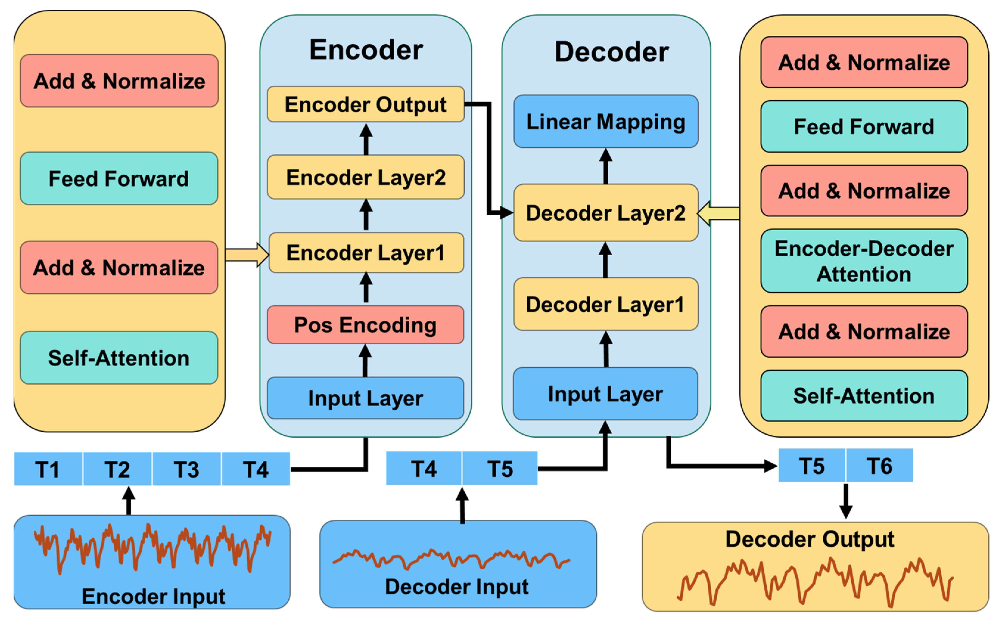
2.2. Prediction with Informer

Time series prediction plays a crucial role in identifying potential faults and taking proactive measures to prevent them, ensuring the safe and stable operation of nuclear steam turbines. By using failure detection and prediction technology, operational efficiency and reliability can be enhanced, maintenance costs reduced, and equipment lifespan extended.

In this section, we propose an informer-based model for time series prediction that incorporates all relevant features across time steps. The input sequence ${\chi }^t=\{x_1^t,\dots ,x_L^t|x_i^t\in R^{d_x}\}$ at time $t$ is processed to predict the output value $y^t=\{y_1^t,\dots ,y_L^t|x_i^t\in R^{d_x}\}$, utilizing an encoding and decoding architecture that enhances the time sequence context’s connection. The Informer model is well suited for processing sequences with extensive time spans and multiple inputs, owing to its ability to capture long-range dependencies among input features and model temporal relationships in the data. The attention mechanism in the informer selectively focuses on the most salient features at each time step, thereby improving prediction accuracy. The encoding and decoding structure ensures that the temporal dependencies between input features are adequately captured for precise time series prediction. The informer model for time series prediction is shown in Figure 1 [13].

The correlation between each query vector $Q$ and the key vector $K$ is computed through the inner product of the two vectors. This correlation is then normalized using the softmax function to obtain the weighted sum of each query vector to all value vectors. The resulting output is a weighted sum of the values that are most relevant to the given query. $Q$ represents the query vector, $K$ represents the key vector, $V$ represents the value vector, and $d_k$ is the dimension of the key vector.

$$Attention(Q,K,V)=softmax(\frac{ Q{K}^T}{\sqrt{d_k}} )V$$

(4)

The input query, key, and value matrices are fed through multi-head attention, where the output of each head attention is concatenated, and finally the output is linearly transformed to obtain the final output. Among them, ${\mathrm{head}}_i=\mathrm{Attention}(Q{W}_i^Q,K{W}_i^K,V{W}_i^V)$ represents the i-th head attention, $W_i^Q,W_i^K,W_i^V$ is the query, key, and value matrix of the i-th head attention, and $W^O$ is the output matrix.

$$MultiHead(Q,K,V)=Concat(hea{d}_{1 },hea{d}_2 ,\cdots ,hea{d}_h )W^O$$

(5)

Positional encoding ensures that the transformer captures positional information in the sequence by adding positional information to the input sequence. Among them, $\mathrm{PE}(pos,2i)$ and $\mathrm{PE}(pos,2i+1)$ indicate that the dimensions on the position $pos$ are $2i$ and $2i+1$. The position encoding value of $d$ is the word vector dimension.

$$P{E}_{(pos,2i) }=sin(\frac{pos}{{10000}^{2i/d}} )$$

(6)

$$P{E}_{(pos,2i=1) }=\cos (\frac{pos}{{10000}^{2i/d}} )$$

(7)

The input sequence is mapped to a high-dimensional continuous vector space through the encoder, and the feature representation of the input sequence is extracted. Then, generate the output sequence through the decoder, receive the feature vector output by the encoder and the previous decoder output, and predict the probability distribution of the next output symbol. Among them, $x$ is the input sequence, and the LayerNorm function is the layer normalization function, $y$ is the input sequence of the decoder, and $z$ is the output sequence of the encoder.

$$Encoder(x)=LayerNorm(x+MultiHead(x,x,x))$$

(8)

$$\begin{array}{c}Decoder(y,z)=LayerNorm(y+MultiHead(y,y,y)\\ +MultiHead(y,z,z))\end{array}$$

(9)

The input vector is processed through a two-layer fully connected network, in which the first layer uses the ReLU activation function, and the second layer directly outputs to obtain the final output vector. Among them, $x$ represents the input vector, $W_1,b_1$ is the weight matrix and bias vector of the first layer, $\max (0,x{W}_1+b_1)$ represents the activation function ReLU of the first layer, $W_2,b_2$ is the weight matrix and bias vector of the second layer, and $\mathrm{FFN}(x)$ represents the output vector.

$$FFN(x)=max(0,x{W}_{1 }+b_1 )W_2 +b_2$$

(10)

Residual connections are used to solve the vanishing gradient problem in deep neural networks. Among them, $x$ represents the input tensor, $\mathrm{Sublayer}$ represents Multi-Head Attention and Feed Forward, and its formula is:

$$LayerNorm(x+Sublayer(x))$$

(11)

The framework of the PT-Informer model for nuclear steam turbine rotor is shown in Figure 2. Compared with traditional frameworks that can only achieve fault detection and classification, it integrates the techniques of fault detection, fault classification, and fault prediction to achieve intelligent diagnosis and prognostics. The data samples are collected through the eddy current displacement sensors and the data acquisition device. The extracted features are then used for fault diagnosis and classification. The prediction module uses the Informer’s encoding and decoding structures to capture the time dependencies between input features and predict potential faults. When faults are predicted, fault detection and fault classification are performed on faults. Cross-validate the model results by cross-referencing and verifying the prediction and detection to ensure the accuracy and reliability of the model. By integrating these techniques, the PT-Informer framework can enable intelligent fault diagnosis and prognostics for nuclear steam turbine rotors, helping to improve operational efficiency, reduce maintenance costs, and extend the equipment’s lifespan.

2.3. Fault Detection with PCA

To elaborate further, PCA [34] is a widely used method for feature extraction that involves transforming the original data matrix into a new space where it can be represented in terms of a smaller number of features or variables. The new space is defined by the principal components, which are linear combinations of the original variables. By selecting a subset of the principal components that explain the most variance in the data, PCA can effectively reduce the dimensionality of the data while retaining the most relevant information. This is achieved by projecting the data onto a lower-dimensional subspace that captures the main patterns and trends in the data, while ignoring the noise and outliers. In the case of fault detection in nuclear steam turbines, PCA can be used to identify the principal components that capture the normal operating behavior of the system, and then monitor deviations from this behavior in real-time to detect potential faults or anomalies. Consider an np data matrix $Y\in R^{n\times m}$, where is consisted of m variables and n samples. So, the $Y$ is decomposed into the following form:

$$Y=t_1{s}_1^{\mathrm{T}}+t_2{s}_2^{\mathrm{T}}+\cdots +t_k{s}_k^{\mathrm{T}}+E=T{S}^{\mathrm{T}}+E$$

(12)

Among them, including the score matrix $T\in R^{n\times h}$, ($h\le m$, $h$ is the number of principal components), the score vector $t_i$, the loading vector $s_i$, and the residual matrix $E$. The key statistics monitored by PCA are given by Hoteling’s $T^2$:

$$T_i^2=t_i{\lambda }^{-1}{t}_i{}^{\mathrm{T}}=x_{i}s{\lambda }^{-1}{s}^{\mathrm{T}}{x}_i{}^{\mathrm{T}}$$

(13)

Hoteling’s $T^2$ statistic is common method in fault detection that measures the overall variation of variables and detect faults when the variation in the latent variables exceeds that of the normal condition. The statistic Q can be defined by:

$$Q_i=e_i^{\mathrm{T}}{e}_i=x_i^{\mathrm{T}}(I-s{s}^{\mathrm{T}}{x}_i)$$

(14)

The Q statistic, also known as SPE, is a measure of the squared prediction error used to evaluate the fit of new samples to a model. The $T^2$ statistic follows an F distribution with a specific level of confidence $\alpha$ (typically 99%). Thus, the statistical $T_{\alpha }^2$ can be expressed as:

$$T_{\alpha }^2=\frac{n(m^2-1)}{m(m-n)}F(n,m-n,\alpha )$$

(15)

The upper limit of the Q statistic, which represents the 100(1−α)% control limit, can be calculated using an F-distribution with $m-n$ degrees of freedom and $F(n,m-n,\alpha )$ chosen level of significance $\alpha$, $m-n$, $\alpha$:

$$Q_{\alpha }={\theta }_1{\left[\frac{{\eta }_{\alpha }\sqrt{2{\theta }_2{l}_0^2}}{{\theta }_1}+1+\frac{{\theta }_2{l}_0(l_0-1)}{{\theta }_1}\right]}^{\frac{1}{l_0}}$$

(16)

The value of ${\theta }_k$ is determined by the sum of the first three eigenvalues of the residual matrix:

$${\theta }_k={\displaystyle \sum _{i=s+1}^m{\lambda }_i^k,(k=1,2,3)}$$

(17)

the intermediate result variable $l_0$:

$$l_0=1-\frac{2{\theta }_1{\theta }_3}{3{\theta }_2^2}$$

(18)

Two statistical indicators, T² and Q, can be used to monitor multiple sources of data in production operations. Figure 3 provides a visual representation of how PCA functions, which can provide a more comprehensive understanding of the process.

The T² statistic can detect sudden abnormal deviations in the variables, such as a mismatch between the actual variable and the base variable, while the Q statistic can detect changes in the new data of the variables. Regions in Figure 3 with data points in the red area indicate abnormal events, which can be used for fault detection. To detect faults using the T² or SPE statistic, the T²-contribution and Q-contribution plots can be employed to assess the significance of each variable. If the value of T² and Q exceeds the predetermined threshold, it indicates the occurrence of a system failure. The SPE plot is defined as follows:

$$SPE={‖\tilde{C}x‖}^2={\displaystyle \sum _{i=1}^{m}Con{t}_i^{SPE}}$$

(19)

$$Con{t}_i^{SPE}=({\gamma }_i^{\mathrm{T}}\tilde{C}x{)}^2$$

(20)

The contribution of each variable to the statistic SPE, $\tilde{C}=I-S{S}^T$ is represented by $Con{t}_i^{SPE}$, ${\gamma }_i^{\mathrm{T}}$ is the i-th column of the identity matrix $H_m$. The T²-contribution plot is defined as:

$$T^2=(x^{T}Rx)={‖R^{\frac{1}{2}}x‖}^2={\displaystyle \sum _{i=1}^{m}Con{t}_i^{T^2}}$$

(21)

$$Con{t}_i^{T^2}={({\gamma }_i^{\mathrm{T}}{R}^{\frac{1}{2}}x)}^2=x^T{R}^{\frac{1}{2}}{\gamma }_i{\gamma }_i^{\mathrm{T}}{R}^{\frac{1}{2}}x$$

(22)

where $R=P^T{\Lambda }^{-1}P$, $i-th$ refers to the $i-th$ column of the identity matrix $H_m$, and $‖\cdot ‖$ can represent the norm in phase space.

After detecting that the T² or SPE has exceeded the threshold, it is possible to identify the contribution of each individual variable to the statistics. The variable with the largest contribution is then considered as the potential fault source, which will serve as input for the subsequent fault prediction model.

2.4. Fault Classification with t-SNE

Fault detection involves identifying whether a system is experiencing any faults or anomalies, while fault classification involves identifying the type of fault that is present. After detecting a fault, fault classification involves categorizing it based on specific classification criteria in order to determine the type and severity of the fault and to provide guidance for fault repair. Typically, fault classification involves extracting features from fault data and applying classification algorithms to accurately identify and classify the type of fault.

After performing feature extraction and dimensionality reduction using PCA and anomaly detection with T² and Q test statistics, t-SNE [35] can be employed for data visualization and clustering in order to classify faults. As a non-linear dimensionality reduction technique, t-SNE projects high-dimensional data into a lower-dimensional space while preserving the relationships among data points as not is shown in Figure 4. This approach offers valuable insights into data distribution and patterns, which can help identify clusters or groups related to different fault types or operating conditions. By assigning labels to clustered data points, a fault classification model can be developed to automatically categorize new data based on similarity to labeled data.

$X=\{x_1,x_2\dots ,x_n\}$ is a high-dimensional spatial feature data set, and $n$ represents the dimension. If $x_i$ and $x_j$ are two features in the high-dimensional feature set, the probability distribution of the two features is the function $p_{j|i}$ and the joint probability density is the $p_{ij}$. The calculation formula is:

$$p_{j|i}=\frac{\exp (-||x_i-x_j{|}^{|2}/2{\sigma }_i^2)}{{\displaystyle \sum _{k\ne i}\exp }(-||x_i-x_k|{|}^2/2{\sigma }_i^2)}$$

(23)

$$p_{ij}=\frac{p_{i|j}+p_{j|i}}{2n}$$

(24)

${\sigma }_i$ is the Gaussian variance centered on $x_i$, determined by binary search.

The high-dimensional space features are reduced to n-dimensional low-dimensional space, and the high-dimensional distribution is replaced by the t-distribution. The degree of freedom of the t-distribution is 1, and the joint probability distribution of the two features $y_i$ and $y_j$ of the low-dimensional space is $q_{ij}$.

$$q_{ij}=\frac{{(1+||y_i-y_j|{|}^2)}^{-1}}{{\displaystyle \sum _{k\ne i}{(1+||y_i-y_k|{|}^2)}^{-1}}}$$

(25)

The KL distance is introduced to measure the similarity of the probability distribution between high and low dimensions, and the KL distance is used to measure the distribution similarity between data points before and after dimension reduction, and the formula of the cost KL divergence is obtained:

$$C={\displaystyle \sum _{i}K}L(P_i||Q_i)={\displaystyle \sum _i{\displaystyle \sum _j{p}_{j|i}}}\log \frac{p_{j|i}}{q_{j|i}}$$

(26)

The KL divergence can be optimized using the gradient descent method, which involves calculating the gradient using the following formula:

$$\frac{\partial C}{\partial y_i}=4{\displaystyle \sum _j(p_{j|i}-q_{j|i})}(y_i-y_j){(1+||y_i-y_j|{|}^2)}^{-1}$$

(27)

During the optimization process, a momentum term is introduced to enhance the direction of gradient descent and expedite the convergence of KL divergence. The formula can be expressed as follows:

$$Y^{(t)}=Y^{(t-1)}+\eta \frac{\delta C}{\delta Y}+\partial (t)(Y^{(t-1)}-Y^{(t-2)})$$

(28)

Among them, $Y^{(t)}$ denotes the KL divergence after the t-th iteration, $\eta$ represents the learning rate, which needs to be pre-defined, and $\partial (t)$ denotes the momentum term.

3. Experiments

3.1. Experiment Setup

In order to validate the effectiveness of the proposed algorithm, a series of experiments were conducted on a set of nuclear steam turbine test rotors to acquire and analyze the vibration signals. We employed eddy current displacement sensors to measure the axial vibration and displacement of the rotor, and utilized the SG8000 data acquisition device for data conditioning, collection, and storage. The collected data included information such as Frequency (sample rate of this wave data), Cycles (the number of revolutions of the rotor), Speed (round per minutes), Samples (total sampling points), and Wave (waveform array). A dataset consisting of 1465 pieces of data was collected for this study, representing five distinct fault types. Each piece contained 1024 array sampling points. The dataset was divided into a training set and a testing set, with 80% (1172 pieces data) used for training purposes and the remaining 20% (293 pieces data) reserved for evaluating the performance of the models. The eddy current displacement sensor is shown in Figure 5a, which is a sensor that measures the displacement of an object based on the eddy current effect. Figure 5b is a SG8000 data-acquisition device, which can be used for data conditioning, acquisition, and storage, and Figure 5c is the experimental nuclear steam turbine rotor.

3.2. Fault Prediction Results

Figure 6 compares the PT-Informer model with the other current advanced prediction model for fault prediction. The y-axis of the turbine current represents the predictions of various models regarding the operational state of the steam turbine. The predicted value PT-informer is represented by red, the predicted value Gated Recurrent Unit(GRU) [36] is represented by brown, the predicted value Long Short-Term Memory(LSTM) [37] is represented by purple, the predicted value Recurrent Neural Network(RNN) is represented by gold, the predicted value Transformer is represented by Magenta color, and the actual value is represented by black.

Table 1. Long sequence time-series forecasting results.

Methods	PT-Informer	GRU	LSTM	RNN	Transformer
R2	0.9960291244	0.9491238937	0.9339795604	0.9144744538	0.9855304990
MAE	0.1707754554	0.5170966758	0.7587701152	1.0483688931	0.3807402089
MSE	0.0853712703	1.0954833102	1.1624907156	1.8177715859	0.2835630504
RMSE	0.2921836243	1.6637348423	1.0781886271	1.3482475981	0.5325063853

and Figure 7 show the performance indicators of different model prediction results, including R2, MAE, MSE, and RMSE. R2 indicates the accuracy of the model fitting data and take a value in the range [0, 1]. The closer the value is to 1, the better the predictive performance of the model. MAE measures the average absolute difference between predicted and actual values, while MSE and RMSE consider squared differences, with RMSE being more interpretable due to sharing the same scale as the original data. The smaller the MAE, MSE, and RMSE indicators, the better the model performs. From the graph, it can be concluded that PT-Informer outperformed the other prediction model in each performance indicators. Specially, PT-Informer outperformed the traditional GRU with a 4.94% improvement in R2 performance for prediction.

3.3. Data Preprocessing

In practical applications, the presence of interference and noise in vibration data poses a significant challenge to signal analysis and fault classification. Therefore, effective feature extraction is required to better capture the useful information in the signal when performing signal analysis and fault classification on long-term vibration data sequences. Fourier transform and wavelet transform are two common signal processing methods, but the selection of a suitable method is problem-dependent. Fourier transform is suitable for stationary periodic signals, while wavelet transform is suitable for non-stationary non-periodic signals. In this paper, we chose wavelet transform as the feature extraction method. Compared with the Fourier transform, wavelet transform exhibited superior time-frequency locality and multi-scale analysis capabilities, enabling it to better capture the detailed characteristics of the signal. We transformed the vibration signal into frequency domain images using wavelet transform and utilized these images as features for the subsequent fault classification task. This approach effectively mitigated noise and interference and improved the accuracy of fault classification.

Figure 8a–e show the original vibration signals and time-frequency diagrams obtained through wavelet transform for different types of fault signals. The faults include rotor fatigue, rotor deformation, rotor unbalance, bearing faults, and oil seal leakage. Rotor fatigue refers to the gradual degradation of structural integrity due to repeated stress cycles. Rotor deformation refers to abnormal deviations from the intended rotor shape. Rotor unbalance occurs when the rotor’s mass distribution is uneven, leading to imbalance during rotation. Bearing faults encompass various issues within the rotor’s bearings. Oil seal leakage refers to the loss of sealing integrity, allowing lubricating oil to escape or contaminants to enter the system. Figure 8f displays the original vibration signals and time-frequency diagram obtained for normal signals. In the wavelet transform time-frequency diagram of normal signals, there is no significant energy signal in the low-frequency, intermediate-frequency, or high-frequency stages. Conversely, the wavelet-transform time-frequency diagrams of other fault signals show a more evident energy signal in the low-frequency, intermediate-frequency, or high-frequency bands. This observation suggests that the fault signal exhibits significant energy concentration or abnormal changes in specific frequency bands, which serves as a crucial basis and valuable clues for fault detection and diagnosis. Through meticulous analysis and comparison of the time-frequency diagrams associated with various fault types, it becomes possible to effectively distinguish and identify different fault modes, thereby providing essential guidance for subsequent fault prediction and diagnosis endeavors.

To evaluate the effectiveness of the feature extraction method, these fault images were clustered using the t-SNE algorithm, with results given in Figure 9. The clustering results demonstrate that the method can effectively differentiate between various fault types, and different types of faults were grouped in separate clusters. This validates the method’s effectiveness and accuracy in the fault classification task.

During experimental analysis, SPE and T² statistics of PT-Informer method were often utilized for fault detection. These two statistics can be used to identify and isolate outliers and noise, as well as to monitor changes within a process. These statistics were calculated for each data point in the Principal Component space, and if a particular sample exceeded a predetermined threshold, it was indicative of an abnormality and warrants further analysis. SPE and T² can also be used for fault diagnosis by analyzing the patterns and trends of the SPE and T² values over time. These statistics are powerful tools for identifying potential problems early on, before they can lead to catastrophic failure, and can help ensure the safe and efficient operation of complex systems.

Figure 10 displays the PT-Informer fault detection results for five different types of faults, with the red lines representing the thresholds for T² and SPE statistics. If the T² or SPE statistics exceeded the threshold, it indicated a fault, and the red dashed rectangle was marked as the fault state. From time 0 to 450, it represents the state at normal time, while from time 450 to 1000, it represents the fault state in order to better show the results, the y-axis values were adjusted to make the difference between SPE and T² under normal and fault conditions more obvious [38].

3.4. Fault Detection Results

After the PT-Informer processing, the results can be fed into a neural network model for classification in fault detection. The neural network can automatically learn the complex nonlinear relationship between input features and fault types, by achieving high-precision fault detection. As shown in Figure 11, the accuracy of the training and validation sets both increased while the loss decreased, indicating the feasibility of this method.

By combining PT-Informer with a neural network, the strengths of both methods can be leveraged to achieve better performance in fault detection. PT-Informer can effectively reduce the dimensionality of high-dimensional data while preserving most of the information, thus simplifying the input for the neural network. Meanwhile, the neural network can capture the complex relationships between features and fault types that may not be easily extracted by PT-Informer alone.

In Figure 12, the confusion matrix illustrates the true and predicted labels, with the numbers in each cell representing the corresponding predicted probabilities. By comparing the confusion matrix diagrams of the PT-Informer and GRU models, it is evident that the PT-Informer model demonstrated superior classification performance in fault diagnosis. The confusion matrices of GRU and PT-Informer used SVC and CNN classifiers, respectively, because PT-Informer has better prediction effect than GRU, so it can generate more accurate data sets, so when using confusion matrix, PT-Informer had a better classification effect. The CNN classifier also had a better classification effect than the SVC classifier. The PT-Informer framework enhanced the fault classification accuracy of nuclear steam turbine rotors from 96.6% to 98% and from 97.4% to 99.6% for different fault types. Furthermore, PT-Informer achieved a perfect classification accuracy of 100% for Type-a faults, Type-C faults, and Fault-e, highlighting its effectiveness in accurately identifying and classifying these specific fault types.

4. Conclusions

This paper presented a novel approach utilizing the PT-Informer framework to learn rotor vibration signals for fault diagnosis and prediction in nuclear steam turbine systems, enabling early detection and diagnosis of potential failures. For the five common faults of nuclear steam turbines, the PT-Informer framework was capable of extracting fault features directly from raw vibration signals, enabling fault detection and fault classification. The results showed that the framework can accurately realize the fault detection and fault classification of nuclear steam turbines. By comparing the prediction performance of the PT-Informer framework with that of the other current advanced models, the superiority of the proposed method over the other advanced models was demonstrated through the analysis of time series prediction graphs and various model performance indicators. Experimental results on a nuclear steam turbine rotor showed that PT-Informer outperformed the traditional GRU model, with a 4.94% improvement in R2 performance for prediction. Furthermore, PT-Informer enhanced the fault classification accuracy from 96.6% to 98% compared to the conventional model. PT-Informer showed significant improvements in prediction performance and fault classification accuracy compared to traditional approaches. While we successfully applied the PT-Informer framework to nuclear steam turbine fault diagnosis and prediction, there remains a question of whether its effectiveness extends to other devices or sensors. In the future, further investigation will be conducted to explore the applicability of the proposed method in various domains, including wind turbines, aero engines, and more.

References

1. Lin, B.; Li, Z. Towards world’s low carbon development: The role of clean energy. Appl. Energy 2022, 307, 118160. [Google Scholar] [CrossRef]
2. Yang, X.; Song, Y.; Wang, G.; Wang, W. A comprehensive review on the development of sustainable energy strategy and implementation in China. IEEE Trans. Sustain. Energy 2010, 1, 57–65. [Google Scholar] [CrossRef]
3. Zhang, F.; Chen, M.; Zhu, Y.; Zhang, K.; Li, Q. A Review of Fault Diagnosis, Status Prediction, and Evaluation Technology for Wind Turbines. Energies 2023, 16, 1125. [Google Scholar] [CrossRef]
4. Tanuma, T. Introduction to steam turbines for power plants. In Advances in Steam Turbines for Modern Power Plants; Woodhead Publishing: Cambridge, UK, 2022; pp. 3–10. [Google Scholar]
5. Li, S.; Li, J. Condition monitoring and diagnosis of power equipment: Review and prospective. High Volt. 2017, 2, 82–91. [Google Scholar] [CrossRef]
6. Salahshoor, K.; Kordestani, M.; Khoshro, M.S. Fault detection and diagnosis of an industrial steam turbine using fusion of SVM (support vector machine) and ANFIS (adaptive neuro-fuzzy inference system) classifiers. Energy 2010, 35, 5472–5482. [Google Scholar] [CrossRef]
7. Jiao, J.; Zhao, M.; Lin, J.; Liang, K. A comprehensive review on convolutional neural network in machine fault diagnosis. Neurocomputing 2020, 417, 36–63. [Google Scholar] [CrossRef]
8. Gao, Z.; Cecati, C.; Ding, S.X. A survey of fault diagnosis and fault-tolerant techniques—Part I: Fault diagnosis with model-based and signal-based approaches. IEEE Trans. Ind. Electron. 2015, 62, 3757–3767. [Google Scholar] [CrossRef]
9. Fenton, W.G.; McGinnity, T.M.; Maguire, L.P. Fault diagnosis of electronic systems using intelligent techniques: A review. IEEE Trans. Syst. Man Cybern. Part C (Appl. Rev.) 2001, 31, 269–281. [Google Scholar] [CrossRef]
10. Ma, J.; Jiang, X.; Han, B.; Wang, J.; Zhang, Z.; Bao, H. Dynamic Simulation Model-Driven Fault Diagnosis Method for Bearing under Missing Fault-Type Samples. Appl. Sci. 2023, 13, 2857. [Google Scholar] [CrossRef]
11. Ni, Q.; Ji, J.C.; Feng, K. Data-driven prognostic scheme for bearings based on a novel health indicator and gated recurrent unit network. IEEE Trans. Ind. Inform. 2022, 19, 1301–1311. [Google Scholar] [CrossRef]
12. Wu, C.; Li, X.; Guo, Y.; Wang, J.; Ren, Z.; Wang, M.; Yang, Z. Natural language processing for smart construction: Current status and future directions. Autom. Constr. 2022, 134, 104059. [Google Scholar] [CrossRef]
13. An, Z.; Cheng, L.; Guo, Y.; Ren, M.; Feng, W.; Sun, B.; Ling, J.; Chen, H.; Chen, W.; Luo, Y.; et al. A Novel Principal Component Analysis-Informer Model for Fault Prediction of Nuclear Valves. Machines 2022, 10, 240. [Google Scholar] [CrossRef]
14. Inyang, U.I.; Petrunin, I.; Jennions, I. Diagnosis of multiple faults in rotating machinery using ensemble learning. Sensors 2023, 23, 1005. [Google Scholar] [CrossRef] [PubMed]
15. Zhong, S.-S.; Fu, S.; Lin, L. A novel gas turbine fault diagnosis method based on transfer learning with CNN. Measurement 2019, 137, 435–453. [Google Scholar] [CrossRef]
16. Lei, Y.; Yang, B.; Jiang, X.; Jia, F.; Li, N.; Nandi, A.K. Applications of machine learning to machine fault diagnosis: A review and roadmap. Mech. Syst. Signal Process. 2020, 138, 106587. [Google Scholar] [CrossRef]
17. Michau, G.; Hu, Y.; Palmé, T.; Fink, O. Feature learning for fault detection in high-dimensional condition monitoring signals. Proc. Inst. Mech. Eng. Part O J. Risk Reliab. 2020, 234, 104–115. [Google Scholar] [CrossRef]
18. Fast, M.; Assadi, M.; De, S. Development and multi-utility of an ANN model for an industrial gas turbine. Appl. Energy 2009, 86, 9–17. [Google Scholar] [CrossRef]
19. Asgari, H.; Chen, X.; Menhaj, M.B.; Sainudiin, R. Artificial neural network–based system identification for a single-shaft gas turbine. J. Eng. Gas Turbines Power 2013, 135, 092601. [Google Scholar] [CrossRef]
20. Barad, S.G.; Ramaiah, P.V.; Giridhar, R.K.; Krishnaiah, G. Neural network approach for a combined performance and mechanical health monitoring of a gas turbine engine. Mech. Syst. Signal Process. 2012, 27, 729–742. [Google Scholar] [CrossRef]
21. Liu, H.; Li, L.; Ma, J. Rolling bearing fault diagnosis based on STFT-deep learning and sound signals. Shock Vib. 2016, 2016, 6127479. [Google Scholar] [CrossRef]
22. Lu, C.; Wang, Z.-Y.; Qin, W.-L.; Ma, J. Fault diagnosis of rotary machinery components using a stacked denoising autoencoder-based health state identification. Signal Process. 2017, 130, 377–388. [Google Scholar] [CrossRef]
23. Tahan, M.; Tsoutsanis, E.; Muhammad, M.; Karim, Z.A. Performance-based health monitoring, diagnostics and prognostics for condition-based maintenance of gas turbines: A review. Appl. Energy 2017, 198, 122–144. [Google Scholar] [CrossRef]
24. Fentaye, A.D.; Ul-Haq Gilani, S.I.; Baheta, A.T.; Li, Y.-G. Performance-based fault diagnosis of a gas turbine engine using an integrated support vector machine and artificial neural network method. Proc. Inst. Mech. Eng. Part A J. Power Energy 2019, 233, 786–802. [Google Scholar] [CrossRef]
25. Zhao, M.; Fu, X.; Zhang, Y.; Meng, L.; Tang, B. Highly imbalanced fault diagnosis of mechanical systems based on wavelet packet distortion and convolutional neural networks. Adv. Eng. Inform. 2022, 51, 101535. [Google Scholar] [CrossRef]
26. Niu, Z.; Zhong, G.; Yu, H. A review on the attention mechanism of deep learning. Neurocomputing 2021, 452, 48–62. [Google Scholar] [CrossRef]
27. Giuliari, F.; Hasan, I.; Cristani, M.; Galasso, F. Transformer networks for trajectory forecasting. In Proceedings of the 2020 25th International Conference on Pattern Recognition (ICPR), Milan, Italy, 10–15 January 2021; pp. 10335–10342. [Google Scholar]
28. Han, K.; Xiao, A.; Wu, E.; Guo, J.; Xu, C.; Wang, Y. Transformer in transformer. Adv. Neural Inf. Process. Syst. 2021, 34, 15908–15919. [Google Scholar]
29. Zhou, H.; Zhang, S.; Peng, J.; Zhang, S.; Li, J.; Xiong, H.; Zhang, W. Informer: Beyond efficient transformer for long sequence time-series forecasting. In Proceedings of the AAAI Conference on Artificial Intelligence, Virtual, 2–9 February 2021; Volume 35, pp. 11106–11115. [Google Scholar]
30. Wu, S.; Xiao, X.; Ding, Q.; Zhao, P.; Wei, Y.; Huang, J. Adversarial sparse transformer for time series forecasting. Adv. Neural Inf. Process. Syst. 2020, 33, 17105–17115. [Google Scholar]
31. Cai, L.; Janowicz, K.; Mai, G.; Yan, B.; Zhu, R. Traffic transformer: Capturing the continuity and periodicity of time series for traffic forecasting. Trans. GIS 2020, 24, 736–755. [Google Scholar] [CrossRef]
32. Xu, M.; Dai, W.; Liu, C.; Gao, X.; Lin, W.; Qi, G.-J.; Xiong, H. Spatial-temporal transformer networks for traffic flow forecasting. arXiv 2020, arXiv:2001.02908. [Google Scholar]
33. Wang, Z.; Zhang, Q.; Xiong, J.; Xiao, M.; Sun, G.; He, J. Fault diagnosis of a rolling bearing using wavelet packet denoising and random forests. IEEE Sens. J. 2017, 17, 5581–5588. [Google Scholar] [CrossRef]
34. Chaouch, H.; Charfeddine, S.; Ben Aoun, S.; Jerbi, H.; Leiva, V. Multiscale monitoring using machine learning methods: New methodology and an industrial application to a photovoltaic system. Mathematics 2022, 10, 890. [Google Scholar] [CrossRef]
35. Tao, H.; Cheng, L.; Qiu, J.; Stojanovic, V. Few shot cross equipment fault diagnosis method based on parameter optimization and feature mertic. Meas. Sci. Technol. 2022, 33, 115005. [Google Scholar] [CrossRef]
36. He, X.; Wang, Z.; Li, Y.; Khazhina, S.; Du, W.; Wang, J.; Wang, W. Joint decision-making of parallel machine scheduling restricted in job-machine release time and preventive maintenance with remaining useful life constraints. Reliab. Eng. Syst. Saf. 2022, 222, 108429. [Google Scholar] [CrossRef]
37. Xiang, L.; Wang, P.; Yang, X.; Hu, A.; Su, H. Fault detection of wind turbine based on SCADA data analysis using CNN and LSTM with attention mechanism. Measurement 2021, 175, 109094. [Google Scholar] [CrossRef]
38. Cheng, L.; An, Z.; Guo, Y.; Ren, M.; Yang, Z.; McLoone, S. MMFSL: A novel multi-modal few-shot learning framework for fault diagnosis of industrial bearings. IEEE Trans. Instrum. Meas. 2023; early access. [Google Scholar] [CrossRef]
Figure 1. The informer model for time series prediction.
Machines 11 00846 g001
Figure 2. Framework of the PT-Informer model for nuclear steam turbine rotor.
Machines 11 00846 g002
Figure 3. Confidence regions for the T2 and Q statistics.
Machines 11 00846 g003
Figure 4. The dimensionality reduction principle of t-SNE.
Machines 11 00846 g004
Figure 5. Nuclear steam turbine testing device: (a) The eddy current displacement sensor, (b) SG8000 data acquisition device, (c) nuclear steam turbine rotor.
Machines 11 00846 g005
Figure 6. Fault prediction in time series data with different methods.
Machines 11 00846 g006
Figure 7. Comparative analysis of model performance metrics for predictive models.
Machines 11 00846 g007
Figure 8. Wavelet transform time-frequency diagram of fault and normal state time series for: (a) rotor fatigue fault, (b) rotor deformation fault, (c) rotor unbalance fault, (d) bearing fault, (e) oil seal leakage fault, and (f) normal signals.
Machines 11 00846 g008aMachines 11 00846 g008b
Figure 9. Fault feature visualization.
Machines 11 00846 g009
Figure 10. Fault detection results of principal component analysis: (a) rotor fatigue fault, (b) rotor deformation fault, (c) rotor unbalance fault, (d) bearing fault, (e) oil seal leakage fault.
Machines 11 00846 g010
Figure 11. Visualization of Training and Validation Accuracy and Loss Curves.
Machines 11 00846 g011
Figure 12. Fault classification results with GRU and PT-Informer: (a) SVC+GRU, (b) SVC+PT-Informer, (c) CNN+GRU, (d) CNN+PT-Informer.
Machines 11 00846 g012