Adaptive Control of M3C-Based Variable Speed Drive for Multiple Permanent-Magnet-Synchronous-Motor-Driven Centrifugal Pumps

Abstract

There has been growing interest in using permanent magnet synchronous motors (PMSMs) for pumping applications to improve energy efficiency. One promising approach for powering these motors in variable speed applications is using an M3C due to its inherent fault tolerance capability. However, M3C converters require a more complex control system than simpler converters. For instance, a basic M3C control system for power transmission requires seventeen PI controllers, whose fixed adjustment depends on the M3C’s dynamical model parameters’ value knowledge, needing initial extensive and time-consuming testing to obtain it. As an alternative, we propose an adaptive M3C control system for variable speed drives powering multiple PMSM-driven centrifugal pumps that reduces the number of controllers to six. Furthermore, the proposal does not require initial knowledge of the converter, motor, or load parameters, making it more practical and versatile. The proposal introduces an ad hoc hybrid passivity-based model reference adaptive controller in cascade with a passivity-based control. It was validated through theoretical stability proof and comparative simulation results with a basic control system under normal and fault operations. As a result, the proposal effectively follows the required rotor speed while enhancing performance by decreasing the current consumption and recovering from a $10\%$ input phase imbalance, a cell short circuit, an open cell, and parameters changes of the motor–pump set.

1. Introduction

1.1. Motivations

The centrifugal pump powered by induction motors (IMs) is widely used to move fluids in various economic sectors. However, its energy consumption is significant compared to other machinery [1]. Therefore, researchers like [1] propose improving the mechanical pump design, while others suggest replacing the IM with more efficient permanent magnet synchronous motors (PMSMs) [2,3,4,5,6]. This manuscript focuses on moving centrifugal pumps with PMSMs.

Using PMSMs is currently a prominent trend in various motor-driving applications due to their low inertia, low noise, high power density, and high efficiency ([7], Section 2.1). They offer the best of both AC (reliable operation benefits) and DC (excellent speed control performance) motors, making them ideal for engineering applications [7,8]. Compared to traditional induction motors (IMs), PMSM motors have demonstrated superior efficiency, as evidenced by ([2], Figure 3). Here, centrifugal pumps driven by PMSMs have a 5%, 8%, and 10% higher efficiency than those driven by IMs for flow rates of 100 m${}^3$/h at 100%, 80%, and 60% speeds, respectively. The works [3,4] propose customizing PMSM design for this application, while [5,6] study a variable speed PMSM for water pumps powered by an AC-AC converter fed by photovoltaic panels. The works [5,6] use a two-level voltage source inverter controlled by model reference adaptive control (MRAC).

The books [9,10] describe the basis of MRAC for the single-input and single-output (SISO) and multiple-input and multiple-output (MIMO) cases, respectively. Based on the concepts given in [9], the work [11] proposes a cascade adaptive passivity-based controller (APBC), and [12] presents a cascade MRAC. This manuscript uses APBC and MRAC techniques together, considering the adaptive control advantages mentioned in ([7], Section 4.5). Furthermore, it applies the direct adaptive control architecture ([7], Figure 20) to an AC-AC converter different than the one used by [5,6].

With the evolution of semiconductors and processors, new power topologies have emerged [13]. The work [14] proposes several fault-tolerant multilevel converters. In this sense, the use of a modular multilevel cascaded converter (MMCC) obtained popularity due to its many benefits, such as redundancy, high efficiency, robustness, lower output voltage TDH, and low maintenance [15,16,17]. Among these converters, the M3C topology is particularly noteworthy and employs smaller floating capacitors [15,18].

Moreover, M3C has inherent fault tolerance characteristics, allowing it to continue proper operations even after having a power supply phase imbalance or power cell failure [15,18]. It ensures energy balancing with low impact on the output currents [18]. Furthermore, it reduces current harmonics, enhances the power factor and efficiency, [15,17,19], eliminates voltage fluctuations, and ensures optimal operation at low output frequencies [20,21]. There are even several studies that propose fault detection and control under a fault of M3C [22,23,24]. This manuscript focuses on controlling the following fault-tolerant M3C used for variable speed drive in PMSM-driven centrifugal pumps.

1.2. Background

Figure 1 shows a commonly used M3C.

An M3C has modularity, the ability to reach high-voltage levels, power quality, bidirectional power conversion, and redundancy [27]. It has nine clusters (three per phase) that link the input phases (a, b, c) with the output phases (r, s, t), each consisting of three cells. Additionally, each cell has a full-bridge monophasic inverter. It has been widely utilized [15]; examples are injecting wind energy into an electrical network [25], in low-frequency AC transmission [28], and as a solid-state transformer for medium- and high-voltage AC substations [29].

However, while having these fault-tolerant capabilities, controlling the M3C is complex compared to simpler converters. Figure 2 describes how the control system of an M3C involves:

• Complex managing of feedback signals that rearrange nine-dimensional measurement vectors $i_{ij}$, $V_{Cij}$, into matrix form to work with variables at an intricate coordinate system called $2\alpha \beta \gamma$, and to later rearrange them back to their vector form to allow for the control [18,26].
• Controlling the average capacitor voltage (ACV) $V_{Cavg}$ in cascade with the input currents amplitude $I_{in}$ control through the required input voltage $v_{in-cl}^{*}$.
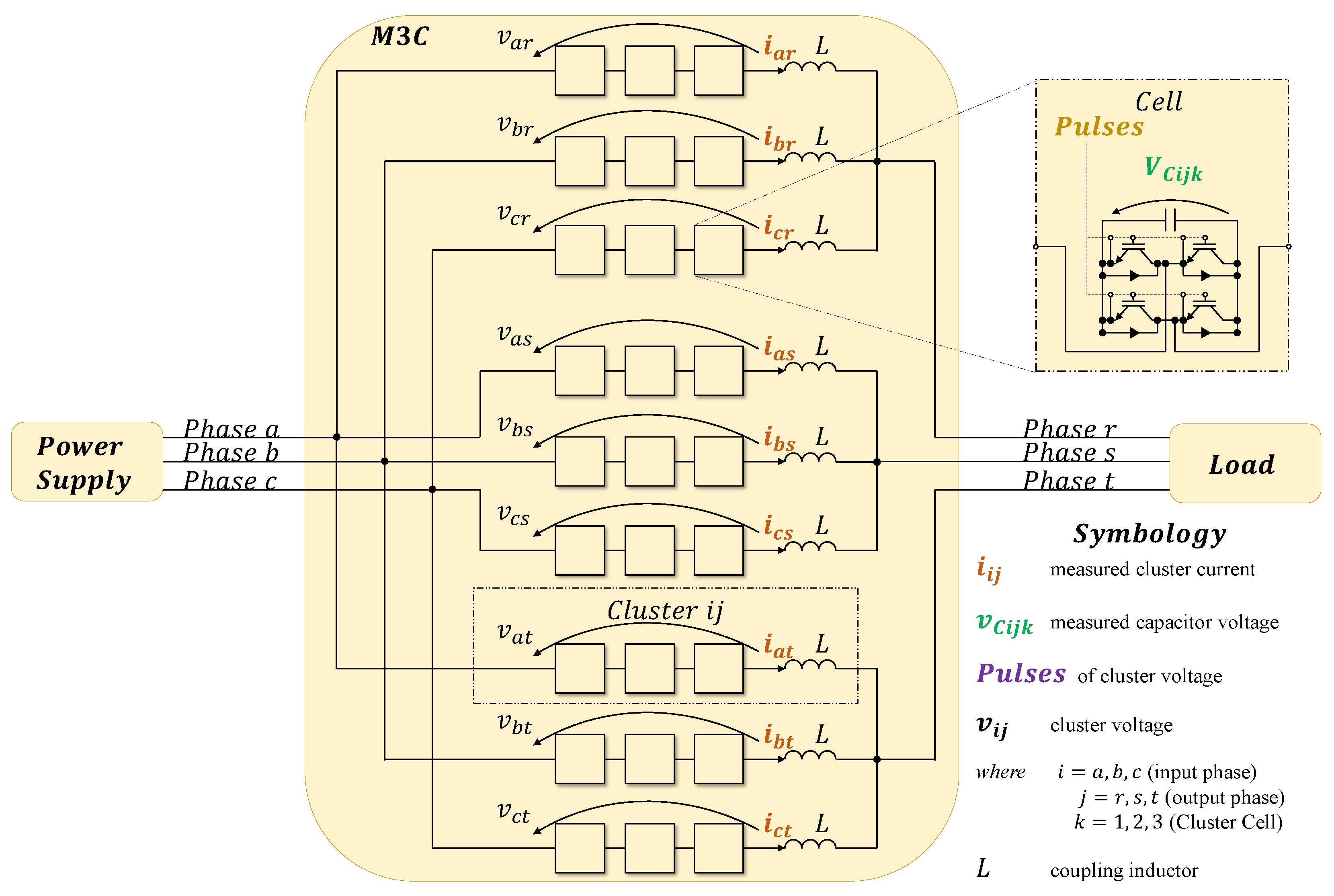
• Keeping zero imbalance of the cluster capacitor voltage (CCV) in cascade with the circulating current $i_{cir}$ control via the needed cluster voltage $v_{cl}^{*}$. It considers reducing the inter-CCV imbalances (CCV imbalance among clusters of different sub-converters) and the intra-CCV imbalances (CCV imbalance among clusters inside the same sub-converters) to zero.
• Controlling a required output variable by adjusting the output voltage $v_{out-cl}^{*}$ amplitude and frequency.

Figure 2. Basic control system of an M3C for transferring energy between the power supply and the load, which is based on [15,26].

Figure 2. Basic control system of an M3C for transferring energy between the power supply and the load, which is based on [15,26].

The control diagram of Figure 2 uses Park transform P [30], $\alpha \beta \gamma$ transform $\mathcal{C}$ [26], double $\alpha \beta \gamma$ transform $\mathcal{C}X{\mathcal{C}}^T$ of different matrix variables X [26], and the combined components transformation matrix $C_D$ [31]. Furthermore, the local cell balancing (LCB) and modulation block may use a phase-shifted (PS) pulse-wide modulation (PWM) technique [21,32], a space vector modulation (SVM) [13], or predictive control [20]. As described below, this manuscript controls an M3C with the most extensively used PS-PWM [15].

1.3. Related Works

Regarding the controllers, the works [19,31] consider that the M3C has several SISO subsystems and use proportional integer (PI) controllers for all variables except for the circulating current. Most reported control strategies for the circulating current regulation are based on a simple P controller [19,31]. However, some authors use a P-resonant (PR) controller as described in [15]. As a result, there are thirteen (13) PI controllers and four (4) PR or P controllers. One (1) PI regulates the ACV direct component in cascade with two (2) PIs for the input current amplitude direct and quadrature components. Eight (8) PIs aim to reduce the CCV imbalance in cascade with four (4) PR or P circulating current controllers. Finally, two (2) PIs regulate the load output current amplitude direct and quadrature components for energy transfer applications between the power supply and the load [15].

The M3C has also been powering electrical motors with an output control strategy that differs from the one shown in Figure 2, and uses a speed control loop. The works [21,26,33] power IMs with an M3C, while [32] drives PMSMs. However, [21,26,32,33] do not describe the used output control strategy. In contrast, ref. [34] (Figure 3a) clearly identifies a field-oriented control (FOC) strategy for an MMCC converter feeding IMs. Moreover, it presents MIMO controllers, significantly reducing the number of controllers. All control systems proposed in [21,26,32,33,34] require an initial estimation of the plant parameters for their adjustment, typically obtained through extensive and time-consuming testing. As an alternative, the following subsection describes our main contributions.

1.4. Contributions

This manuscript proposes an MIMO adaptive control of an M3C-based variable speed drive. It operates multiple PMSM-driven centrifugal pumps using a scalar control scheme ($V/f$) [35] for the output control, as FOC is unnecessary in pumping applications. Our proposal involves the following novelties:

• Obtaining the multivariable M3C state-space model for control. It is an MIMO dynamical system with a currents inner loop, a voltages outer loop, and an inner–outer interface. Appendix A of this manuscript details the model obtained, which complements, describes, rearranges, and summarizes elements taken from [15,26,28]. In contrast to [15,26,28], herein, we give details for control implementation, such as the matrix and vector operations (please see, for instance, the managing feedback signals details given in Figure 2), and identify the state-space model form with inner and outer loops.
• Using MIMO adaptive controllers instead of non-adaptive SISO controllers [19,31,34]. We show that it is a viable and more straightforward solution. The proposal gains the benefits discussed in [34] of reducing the number of controllers by using an MIMO approach for an MMCC but herein for the M3C. In contrast to the works [19,31,34], tuning adaptive controllers does not require an initial estimation of the plant parameters, decreasing the commissioning time. Moreover, they adapt to plant changes without compromising their effectiveness.
• Proposing a passivity-based hybrid MRAC called PBMRAC. In contrast to [5,6,9], it uses the MRAC as a low-pass filter for the noisy reference input signals. Moreover, PBMRAC introduces to MRAC a term of an adaptive passivity-based controller (APBC) [11] to attend to the closed-loop system response time. M3C control particularly needs it after having inner reference input noise periods more than sixty times distant from the M3C inner time constant.
• Presenting APBC in cascade with PBMRAC. It expands the cascade MRAC [12] and the cascade APBC [11]. The first uses an outer SISO controller, whereas the M3C outer loop requires an MIMO controller. Moreover, as Figure 2 shows, the M3C has zero or constant outer references, eliminating the need for the outer reference model; therefore, an outer APBC [11] ensures a faster outer loop’s time response.

The following manuscript sections describe the control preliminaries in Section 2. Section 3 details the proposed adaptive control algorithm. Section 4 exhibits the experimental setup and obtained results illustrating the proposal’s effectiveness. Finally, the authors present concluding remarks in Section 5.

2. Preliminaries

This section commences by introducing the mathematical model of the plant to be controlled, the M3C. This modeling is necessary for the controllers’ design. Subsequently, it presents the conventional PI tuning methods, having the issue of a significant number of controllers. Finally, it gives the requisite background information of the cascade MRAC to be extended with the proposal to decrease the number of controllers, among other advantages.

2.1. M3C State-Space Model

The M3C state-space model obtained is detailed in Appendix A, resulting in Equations (A7) and (A13). The following dynamical equations describe it:

$$2\alpha \beta \gamma \text{ Currents Inner Loop}$$

$$\begin{array}{cc}{\dot{I_{Lin}}}_{-cl}\left(t\right)=-\frac{\sqrt{3}}{L}{V}_{in-cl}\left(t\right)+{\mathsf{\Delta }}_{in-cl}\left(t\right),\hfill & \hfill \text{Input current amplitude}\\ {\dot{i_{cir}}}_{-cl}\left(t\right)=-\frac{1}{L}{v}_{cl}\left(t\right),\hfill & \hfill \text{Circulating alternating current}\\ {\dot{I_{out}}}_{-cl}\left(t\right)=-\frac{1}{L}{V}_{out-cl}\left(t\right)+{\mathsf{\Delta }}_{out-cl}\left(t\right),\hfill & \hfill \text{Output current amplitude}\end{array}$$

(1)

$$2\alpha \beta \gamma \text{ Inner–Outer Interface}$$

$$\begin{array}{c}{I}_{Lin-cl}\left(t\right)={\left[I_{Lin-cl\_d}\left(t\right)0\right]}^T,\hfill \\ i_{cir-cl}\left(t\right)=C_D^{-1}\left\{T_r^{-1}\left[\begin{array}{c}P{(-{\theta }_{in})}^{-1}\\ P{\left({\theta }_{in}\right)}^{-1}\end{array}\right]I_{cir1}\left(t\right)+\left[\begin{array}{c}P{(-{\theta }_{out})}^{-1}\\ P{\left({\theta }_{in}\right)}^{-1}\end{array}\right]I_{cir2}\left(t\right)\right\},\hfill \end{array}$$

(2)

$$2\alpha \beta \gamma \text{ Voltages Outer Loop}$$

$$\begin{array}{cc}{\dot{V}}_{Cavg}\left(t\right)=\frac{V_{avg}\left(t\right)}{3Cϵ\left(t\right)V_C^{*}}{I}_{Lin-cl\_d}\left(t\right)+{\mathsf{\Delta }}_{avg}\left(t\right),\hfill & \hfill \text{ACV amplitude}\\ {\dot{V}}_{Cintra}\left(t\right)=\frac{V_{intra}{\left(t\right)}^T}{\sqrt{6}Cϵ\left(t\right)V_C^{*}}{T}_r{I}_{cir1}\left(t\right)+{\mathsf{\Delta }}_{intr{a}_{C_D}}\left(t\right),\hfill & \hfill \text{Intra-CCV imbalance amplitude}\\ {\dot{V}}_{Cinter}\left(t\right)=\frac{V_{inter}{\left(t\right)}^T\left(t\right)}{\sqrt{3}Cϵ\left(t\right)V_C^{*}}{I}_{cir2}\left(t\right)+{\mathsf{\Delta }}_{inter}\left(t\right),\hfill & \hfill \text{Inter-CCV imbalance amplitude}\end{array}$$

(3)

where, in the inner loop, the output variables to control are the amplitudes of the input and output cluster currents $I_{in-cl}\in {\Re }^{2\times 1}$ and $I_{out-cl}\in {\Re }^{2\times 1}$, and the instantaneous circulating current $i_{cir-cl}\in {\Re }^{4\times 1}$. Here, the input variables are the amplitudes of the input and output voltages $V_{in-cl}\in {\Re }^{2\times 1}$ and $V_{out-cl}\in {\Re }^{2\times 1}$, and the instantaneous cluster voltage $v_{cl}\in {\Re }^{4\times 1}$. The parameter is the coupling inductors inductance L. Finally, the time-varying and bounded disturbance terms for the input are ${\mathsf{\Delta }}_{in-cl}\left(t\right)=\frac{3}{L}{ϵ}_{in}\left(t\right)V_{in\_rated}\in {\Re }^{2\times 1}$ and ${\mathsf{\Delta }}_{out-cl}\left(t\right)=-\frac{\sqrt{3}}{L}{ϵ}_{out}\left(t\right)V_{out\_rated}\in {\Re }^{2\times 1}$ for the output currents, where ${ϵ}_{in}\left(t\right)$ and ${ϵ}_{out}\left(t\right)$ are rated voltages fluctuations.

For the outer loop, the output variables are the ACV $V_{Cavg}\in \Re$, the intra-CCV imbalance $V_{Cintra}\in {\Re }^{4\times 1}$, and the inter-CCV imbalance $V_{Cinter}\in {\Re }^{4\times 1}$. The input variables are the amplitudes of the cluster input direct component $I_{in-cl\_d}\in \Re$ and the circulating currents $I_{cir1}\in {\Re }^{4\times 1}$ and $I_{cir2}\in {\Re }^{4\times 1}$. There are also time-varying bounded disturbance terms ${\mathsf{\Delta }}_{avg}\left(t\right)\in \Re$, ${\mathsf{\Delta }}_{intr{a}_{C_D}}\left(t\right)\in {\Re }^{4\times 1}$, and ${\mathsf{\Delta }}_{inter}\left(t\right)\in {\Re }^{4\times 1}$. Finally, the fixed parameters are the cells capacitor capacitance C and required capacitor voltage $V_C^{*}\in \Re$, while the time-varying parameters are the cluster voltages amplitudes $V_{intra}\left(t\right)\in {\Re }^{4\times 1}$, $V_{inter}\left(t\right)\in {\Re }^{4\times 1}$, $V_{avg}\left(t\right)\in \Re$ and the capacitor voltage fluctuations $ϵ\left(t\right)$.

The inner–outer interface links the direct component of the line input cluster current $I_{Lin-cl\_d}$ with the input cluster current $I_{in-cl}$. Moreover, it relates the circulating current amplitudes $I_{cir1}$ and $I_{cir2}$ with the instantaneous circulating current $i_{cir-cl}$, after using the auxiliary transformation matrix $C_D$ [31] and the Park transformation matrix P [30] with the corresponding input ${\theta }_{in}$ and output ${\theta }_{out}$ angles dependence. Please see Appendix A and Figure 2 for details.

Regarding the operating points in this $2\alpha \beta \gamma$ coordinate, the outer loops consider an ACV setpoint of $V_{Cavg}^{*}=3V_C^{*}$ ([26], definition given below in Equation (26)), working at zero intra-CCV imbalance $V_{Cintr{a}_{C_D}}^{*}=0$ and zero inter-CCV imbalance $V_{Cinter}^{*}=0$ [15]. Moreover, the output current reference would be $I_{out-cl}^{*}=\frac{sqrt\left(3\right)}{3}{I}_{out}$ for applications of energy transference between the power supply and the load ([15], Equation (24)).

The following section describes the PI controllers design for the M3C converter.

2.2. Basic Control Based PI Controllers

PI controllers design starts by assuming that plant parameters are constant; thus, ${ϵ}_{in}\left(t\right)={ϵ}_{out}\left(t\right)=ϵ\left(t\right)=1$. Later, the method splits every Equations (1)–(3) into scalar subsystems, each one having the general form $\dot{y}\left(t\right)=b·u\left(t\right)+\delta \left(t\right)$. Here, $y\left(t\right)\in \Re$ is the output variable, $u\left(t\right)\in \Re$ is the input, b represents the fixed subsystems parameter, and $\delta \left(t\right)$ is the disturbance.

Then, Laplace transform is applied, obtaining $Y\left(S\right)=\left(\frac{b}{S}\right)(U\left(S\right)+b^{-1}\mathsf{\Delta }\left(S\right)$, not including the circulating current working in alternating current. Here, the corresponding open-loop transfer function is $F{T}_{LA}\left(S\right)=\frac{b}{S}$ after neglecting the disturbance term, i.e., $\mathsf{\Delta }\left(S\right)=0$.

After considering the PI transfer function $(K_p+\frac{K_i}{S})$ acting in series with the $F{T}_{LA}$, the feed forward transfer function is $G\left(S\right)=(K_p+\frac{K_i}{S})\left(\frac{b}{S}\right)$. Later, considering the feedback transfer function $H\left(S\right)$, one may obtain the following closed-loop transfer function as [36]:

$$F{T}_{LC}=\frac{G\left(S\right)}{1+G\left(S\right)H\left(S\right)}=\frac{K_{p}b·S+K_{i}b}{S^2+K_{p}b·S+K_i·b}=\frac{2\xi {\omega }_{n}S+{\omega }_n^2}{S^2+2\xi {\omega }_{n}S+{\omega }_n^2},$$

(4)

where $\xi$ is the damping coefficient and ${\omega }_n$ is the natural frequencies in $rad/s$.

The feedback sensor transfer function $H\left(S\right)$ is often considered a unitary gain. Moreover, we can identify in (4) the equivalence terms $2\xi {\omega }_n=K_{p}b$ and ${\omega }_n^2=K_{i}b$ between the general second-order equation of the right side and the obtained result of the center side. This allows for adjusting the PI controllers as follows:

$$\begin{array}{c}\hfill u\left(t\right)={\theta }^T\omega \left(t\right)=\left[K_p{K}_i\right]\left[\begin{array}{c}e\left(t\right)\\ {\int }_0^{t}e\left(\tau \right)d\tau \end{array}\right],\mathrm{with}{K}_p=\frac{2\xi {\omega }_n}{b}\mathrm{and}{K}_i=\frac{{\omega }_n^2}{b}.\end{array}$$

(5)

To tune the fixed parameters ${\theta }^T$ of PI controllers based on (5), $\xi =\frac{\sqrt{2}}{2}$ is usually considered ([36], Section (5-3)). However, there are different values of b, ${\omega }_n$, and PI quantities for the distinct controlled variables, as

Table 1. Values of b and ${\omega }_n$ for each controller.

Controller	b	${\mathit{\omega }}_{\mathit{n}}$	PI Quantity
Input Current Amplitude Control $dq$	$-\frac{\sqrt{3}}{L}$	$2\pi \left(f_{in}\right)$	2
ACV Control d	$\frac{V_{avg}}{3C{V}_C^{*}}$	$2\pi$ (1 Hz)	1
Intra-CCV Imbalance Control	$\frac{V_{i{n}_{\alpha }}}{\sqrt{6}C{V}_C^{*}}$	$2\pi$ (5 Hz)	4
Inter-CCV Imbalance Control $\alpha \gamma$	$-\frac{V_{ou{t}_{\alpha }}}{\sqrt{3}C{V}_C^{*}}$	$2\pi$ (5 Hz)	1
Inter-CCV Imbalance Control $\beta \gamma$	$\frac{V_{ou{t}_{\alpha }}}{\sqrt{3}C{V}_C^{*}}$	$2\pi$ (5 Hz)	1
Inter-CCV Imbalance Control $\gamma \alpha \beta$	$\frac{V_{i{n}_{\alpha }}}{\sqrt{3}C{V}_C^{*}}$	$2\pi$ (5 Hz)	2

shows. Two (2) identical PIs regulate the input and output current amplitude components d and q with $b=-\frac{\sqrt{3}}{L}$, as described in (1) and (A7). One (1) PI controls the ACV with $b=\frac{V_{avg}}{3C{V}_C^{*}}$ as can be seen in (3) and (A14). Four (4) PIs control the intra-CCV imbalance, where $V_{intra}=V_{i{n}_{\alpha }}{\left[\begin{array}{cccc}1& 1& 1& 1\end{array}\right]}^T$ from (A14); thus, all components of the vector $V_{intra}$ are equal to $V_{i{n}_{\alpha }}$, having the same $b=\frac{V_{intra}^T}{\sqrt{6}C{V}_C^{*}}$. Finally, also four (4) PIs control the inter-CCV imbalance. However, these have different values of b as described in Table 1 due to $V_{inter}={\left[\begin{array}{cccc}-V_{ou{t}_{\alpha }}& V_{ou{t}_{\alpha }}& V_{i{n}_{\alpha }}& V_{i{n}_{\alpha }}\end{array}\right]}^T$ from (A14).

The alternating circulating current controller often considers four (4) P controllers adjusted as in (5) but $k_i=0$ [37], and, in our case, $b=-\frac{1}{L}$ and ${\omega }_n=2\pi \left(10f_{out}\right)$.

Finally, for applications of energy transference between the power supply and the load [15,26], the output current amplitude control $dq$ would have two PI controllers adjusted as in (5) and considering $b=-\frac{1}{L}$ and ${\omega }_n=2\pi \left(f_{out}\right)$.

Remark 1.

It is imperative to estimate the plant parameters value ${\theta }^T$ to adjust the PI controllers, as seen in Equation (5) and Table 1. This knowledge is usually obtained through initial extensive testing, which can be time consuming (please see [38] as an example for IMs). It is also crucial for the controllers to handle plant changes without compromising their effectiveness. For example, robustness is needed to handle the disturbances shown in Equations (1) and (3) and model uncertainties or unmodeled dynamics such as those of the cell inverters considered as a transfer function $K/(1+\tau S)$ and causing a delay of minimum $5\times Tau$.

Finally, the output controller must be adjusted as we study pumping applications. Thus, the following P controller, called a scalar control scheme ($V/f$), is commonly used for a two-level voltage source inverter feeding PMSD-driven centrifugal pumps ([35], Equation (1)):

$$V_{out-cl\_d}^{*}=\left\{\begin{array}{cc}0\hfill & \mathrm{for} 0<{\omega }_r<{\omega }_{r\_min}\hfill \\ P_1{\omega }_r^{*}+\sqrt{2}{V}_{boost},\mathrm{with} P_1=\sqrt{2}(\frac{V_{s\_rated}}{{\omega }_{r\_rated}}-\frac{V_{boost}}{{\omega }_{r\_c}})\hfill & \mathrm{for} {\omega }_{r\_min}<{\omega }_r<{\omega }_{r\_c}.\hfill \\ P_2{\omega }_r^{*},\mathrm{with} P_2=\sqrt{2}\frac{V_{s\_rated}}{{\omega }_{r\_rated}}\hfill & \mathrm{for} {\omega }_{r\_c}<{\omega }_r<{\omega }_{r\_rated}\hfill \end{array}\right.$$

(6)

Here, $V_{s\_rated}$ is the rated phase voltage from the motor data plate. ${\omega }_{r\_rated}$ is the motor-rated rotor speed in $rad/s$. The $V_{boost}$ is a controller bias or offset (with a value up to $50\%$ of $V_{s\_rated}$) allowing the PMSM to deliver a certain amount of starting torque. The $V_{boost}$ operates from minimum frequency ${\omega }_{r\_min}$ (with a value up to $6\%$ of ${\omega }_{r\_rated}$) to the cut-frequency ${\omega }_{r\_c}$ (with a value up to $50\%$ of ${\omega }_{r\_rated}$) [35].

Remark 2.

In order to attain the desired rotor angular frequency ${\omega }_r^{*}$ with a ramp-up, a two-level voltage source inverter necessitates a phase stator voltage amplitude of $V_{out-cl}^{*}={\left[V_{out-cl\_d}^{*}0\right]}^T$. However, the output voltage required for the M3C is in $double\alpha \beta \gamma$ coordinates, utilizing a power invariant transformation [39] in lieu of Clarke’s transformation that preserves the amplitude [40]. This paper proposes utilizing Equation (6) ([35], Equation (1)) in conjunction with the subsequent equation:

$$V_{out-cl}^{*}=\sqrt{3}{\left[V_{out-cl\_d}^{*}0\right]}^T$$

(7)

The following section will give an overview of an adaptive controller that can maintain optimal performance while adapting to plant changes without requiring knowledge of plant parameters.

2.3. Cascade Adaptive Control Background

The M3C modeled as (1) to (3) needs a cascade control system and the following cascade MRAC ([12], Equations (14)–(22)) ensures the outputs $y_o$ and $y_i$ tracks the references $y_o^{*}$ and $y_i^{*}$:

$$\begin{array}{cc}{\dot{y}}_{ro}\left(t\right)=-a_{ro}{y}_{ro}\left(t\right)+b_{ro}{y}_o^{*}\left(t\right),\hfill & \hfill \text{Outer reference model}\\ u_o\left(t\right)=-{\theta }_o{\left(t\right)}^T{\omega }_o\left(t\right),\hfill & \hfill \text{Outer adaptive control law}\\ {\omega }_o\left(t\right)={\left[\begin{array}{ccc}{y}_o\left(t\right)& f_2(u;I,y_i)& y_o^{*}\left(t\right)\end{array}\right]}^T,\hfill & \hfill \text{MRAC outer information vector}\\ {\dot{\theta }}_o{\left(t\right)}^T=-(sign\left(b_o\right)e_o\left(t\right){\omega }_o{\left(t\right)}^T+{\sigma }_o{\theta }_o{\left(t\right)}^T){\mathrm{\Gamma }}_o,\hfill & \hfill \text{Outer adaptive law for MRAC}\\ {\theta }_o^{*}{\left(t\right)}^T=\left[\begin{array}{ccc}{b}_o^{-1}\left(t\right)a_{ro}& b_o^{-1}\left(t\right)a_o& -b_o^{-1}\left(t\right)b_{ro}\end{array}\right],\hfill & \hfill \text{Ideal outer MRAC parameter}\end{array}$$

(8)

$$\begin{array}{cc}{y}_i^{*}\left(t\right)=f_1\left(u_o\left(t\right)\right),\hfill & \hfill \text{Inner-outer loop interface}\end{array}$$

(9)

$$\begin{array}{cc}{\dot{y}}_{ri}\left(t\right)=-A_{ri}{y}_{ri}\left(t\right)+B_{ri}{y}_i^{*}\left(t\right),\hfill & \hfill \text{Inner reference model}\\ u_i\left(t\right)=-{\theta }_i{\left(t\right)}^T{\omega }_i\left(t\right),\hfill & \hfill \text{Inner adaptive control law}\\ {\omega }_i\left(t\right)={\left[\begin{array}{ccc}{y}_i{\left(t\right)}^T& 1_m^T& y_i^{*}{\left(t\right)}^T\end{array}\right]}^T,\hfill & \hfill \text{MRAC inner information vector}\\ {\dot{\theta }}_i{\left(t\right)}^T=-(sign\left(B_i\right)e_i\left(t\right){\omega }_i{\left(t\right)}^T+{\sigma }_i{\theta }_i{\left(t\right)}^T){\mathrm{\Gamma }}_i,\hfill & \hfill \text{Inner adaptive law for MRAC}\\ {\theta }_i^{*}{\left(t\right)}^T=\left[\begin{array}{ccc}{B}_i^{-1}{A}_{ri}& B_i^{-1}{A}_i\left(t\right)& -B_i^{-1}{B}_{ri}\end{array}\right].\hfill & \hfill \text{Ideal inner MRAC parameter}\end{array}$$

(10)

Here, the outer tracking error is $e_o\left(t\right)=y_{ro}\left(t\right)-y_o\left(t\right)\in \Re$ and the inner tracking error is $e_i\left(t\right)=y_{ri}\left(t\right)-y_i\left(t\right)\in {\Re }^m$. The variables $y_{ro}\left(t\right)\in \Re$, $y_{ri}\left(t\right)\in {\Re }^m$ are the outer and inner reference model outputs. The set points are $y_o^{*}\left(t\right)\in \Re$ and $y_i^{*}\left(t\right)\in {\Re }^m$. The reference model parameters are $a_{ro},b_{ro}\in \Re$ and $A_{ri},B_{ri}\in {\Re }^{(m\times m-Diagonal)}$, made equal ($a_{ro}=b_{ro}$ and $A_{ri}=B_{ri}$) for an exact set point tracking without scaling. The adaptive external and internal controllers $u_o\left(t\right)\in \Re$ and $u_i\left(t\right)\in {\Re }^m$ depend on their adaptive parameters ${\theta }_o\left(t\right)\in {\Re }^3$ and ${\theta }_i\left(t\right)\in {\Re }^{(m\times 3m)}$ and their corresponding information vectors ${\omega }_o\left(t\right)\in {\Re }^3$ and ${\omega }_i\left(t\right)\in {\Re }^{3m}$. The ideal adaptive parameters are ${\theta }_o^{*}\left(t\right)\in {\Re }^3$ and ${\theta }_i^{*}\left(t\right)\in {\Re }^{(m\times 3m)}$. The term $1_m\in {\Re }^m$ refers to a vector with all its components equal to one. Besides the model reference parameters, the cascade MRAC has the following tuning parameters: adaptive law fixed-gains ${\mathrm{\Gamma }}_o\in {\Re }^{(3\times 3-Diagonal)}$ and ${\mathrm{\Gamma }}_i\in {\Re }^{(3m\times 3m-Diagonal)}$, and adaptive law modification factors ${\sigma }_o\in \Re$ and ${\sigma }_i\in {\Re }^{(3m\times 3m-Diagonal)}$.

Cascade MRAC (8)–(10) applies to time-varying cascade systems of the following form ([12], Equations (11)–(13)):

$$\begin{array}{cc}{\dot{y}}_i\left(t\right)=A_i\left(t\right)+B_i\left(t\right)·u_i\left(t\right),\hfill & \hfill \text{Inner loop}\\ y_i\left(t\right)=f_1\left(u_o\left(t\right)\right),\hfill & \hfill \text{Inner-outer interface}\\ {\dot{y}}_0\left(t\right)=a_o\left(t\right)f_2(u;I,y_i)+b_o\left(t\right)·u_o\left(t\right),\hfill & \hfill \text{Outer loop}\end{array}$$

(11)

where $y_o\left(t\right)\in \Re$ and $y_i\left(t\right)\in {\Re }^m$ are the outer and inner output variables, respectively. The inputs are $u_o\left(t\right)\in \Re$ for the outer loop and $u_i\left(t\right)\in {\Re }^m$ for the inner loop. Moreover, $a_o\left(t\right),b_o\left(t\right)\in \Re$ and $A_i\left(t\right),B_i\left(t\right)\in {\Re }^{m\times m}$ are time-varying plant parameters, where $B_i\left(t\right)=|B_i\left(t\right)|Sign\left(B_i\left(t\right)\right)$ and $b_0\left(t\right)=|b_0\left(t\right)|Sign\left(b_0\left(t\right)\right)$, with $|B_i\left(t\right)|$ and $|b_0\left(t\right)|$ the modulus of each element of $B_i\left(t\right)$ and $b_0\left(t\right)$.

Remark 3.

It is important to note that the cascade MRAC (8)–(10) uses an outer SISO controller, whereas the M3C outer loop (3) requires an MIMO controller. Additionally, Figure 2 shows that the M3C has zero or constant outer references, eliminating the need for the outer reference model of (8), which would slow down the outer loop’s time response. Finally, the inner control loop receives noisy reference input signals with certain switching noise periods. Although the inner reference model of (10) could filter these signals, it would disregard the required inner loop response time, failing to ensure both needs.

These issues are solved by the controller proposed in the following section.

3. Proposal

Based on the previously described preliminaries, this section proposes an adaptive controller that solves the cascade MRAC issue identified in Remark 3 and decreases the number of controllers. It applies to the following system that encompasses the M3C state-space model (1)–(3) introduced in Section 2.1:

$$\begin{array}{cc}\dot{y_i}\left(t\right)=B_i\left(t\right)u_i\left(t\right)+{\mathsf{\Delta }}_i\left(t\right),\hfill & \hfill \text{Inner loop}\\ y_i\left(t\right)=f_1\left(u_o\left(t\right)\right),\hfill & \hfill \text{Inner-outer interface}\\ \dot{y_0}\left(t\right)=B_o\left(t\right)u_o\left(t\right)+{\mathsf{\Delta }}_o\left(t\right),\hfill & \hfill \text{Outer loop}\end{array}$$

(12)

where $y_o\left(t\right)\in {\Re }^n$ and $y_i\left(t\right)\in {\Re }^m$ are the outer and inner output variables, respectively. The outer control input is $u_o\left(t\right)\in {\Re }^n$ and the inner is $u_i\left(t\right)\in {\Re }^m$. Moreover, $B_o\left(t\right)\in {\Re }^{n\times n}$ and $B_i\left(t\right)\in {\Re }^{m\times m}$ are time-varying and unknown plant parameters, where $B_i\left(t\right)=|B_i\left(t\right)|Sign\left(B_i\left(t\right)\right)$ and $B_0\left(t\right)=|B_0\left(t\right)|Sign\left(B_0\left(t\right)\right)$. Here, the matrixes $|B_i\left(t\right)|$ and $|B_0\left(t\right)|$ are composed by the modulus of each element of $B_i\left(t\right)$ and $B_0\left(t\right)$ and are unknown. Furthermore, the matrix $Sign\left(B_i\left(t\right)\right)$ and $Sign\left(B_0\left(t\right)\right)$ are composed by the sign of each element of $B_i\left(t\right)$ and $B_0\left(t\right)$ and are known. The known interface nonlinear function is $f_1\in {\Re }^{m\times n}$. Finally, ${\mathsf{\Delta }}_i\left(t\right)$ and ${\mathsf{\Delta }}_o\left(t\right)$ are the inner and outer bounded and unknown disturbances, respectively.

The following theorem describes the proposal:

Theorem 1.

For systems of the form (12), the following adaptive controller ensures that the outputs $y_o$ and $y_i$ tend to the constant references $y_o^{*}$ and $y_i^{*}$, respectively:

$$\begin{array}{cc}{u}_o\left(t\right)=-{\theta }_o{\left(t\right)}^T{\omega }_o\left(t\right),\hfill & \hfill \mathit{Outer} \mathit{control} \mathit{law}\\ {\omega }_o\left(t\right)={\left[\begin{array}{cc}{\mathsf{\Delta }}_{o\_b}^T& u_o^p{\left(t\right)}^T\end{array}\right]}^T,\hfill & \hfill \mathit{APBC} \mathit{outer} \mathit{information} \mathit{vector}\\ \mathit{with}{u}_o^p\left(t\right)=K_o\nabla V_{e_o}\left(t\right),\hfill \\ \dot{{\theta }_o}{\left(t\right)}^T=-(sign\left(b_o\right)\nabla V_{e_o}\left(t\right){\omega }_o{\left(t\right)}^T+{\sigma }_o{\theta }_o{\left(t\right)}^T){\mathrm{\Gamma }}_o,\hfill & \hfill \mathit{APBC} \mathit{outer} \mathit{adaptive} \mathit{law}\\ {\theta }_o^{*}{\left(t\right)}^T=\left[\begin{array}{cc}{B}_o^{-1}\left(t\right)& B_o^{-1}\left(t\right)\end{array}\right],\hfill & \hfill \mathit{Ideal} \mathit{outer} \mathit{APBC} \mathit{parameter}\end{array}$$

(13)

$$\begin{array}{cc}{y}_i^{*}\left(t\right)=f_1\left(u_o\left(t\right)\right),\hfill & \hfill \mathit{Inner}\text{-}\mathit{outer} \mathit{loop} \mathit{interface}\end{array}$$

(14)

$$\begin{array}{cc}{\dot{y}}_{ri}\left(t\right)=-A_{ri}{y}_{ri}\left(t\right)+B_{ri}{y}_i^{*}\left(t\right),\hfill & \hfill \mathit{Inner} \mathit{reference} \mathit{model}\\ u_i\left(t\right)=-{\theta }_i{\left(t\right)}^T{\omega }_i\left(t\right),\hfill & \hfill \mathit{Inner} \mathit{control} \mathit{law} \mathit{based}\\ {\omega }_i\left(t\right)={\left[\begin{array}{cccc}{y}_i{\left(t\right)}^T& y_i^{*}{\left(t\right)}^T& {\mathsf{\Delta }}_{i\_b}^T& u_i^p{\left(t\right)}^T\end{array}\right]}^T,\hfill & \hfill \mathit{PBMRAC} \mathit{inner} \mathit{inform}. \mathit{vector}\\ \mathit{with}{u}_i^p\left(t\right)=K_i\nabla V_{e_i}\left(t\right),\hfill \\ \dot{{\theta }_i}{\left(t\right)}^T=-(sign\left(B_i\right)\nabla V_{e_i}\left(t\right){\omega }_i{\left(t\right)}^T+{\sigma }_i{\theta }_i{\left(t\right)}^T){\mathrm{\Gamma }}_i,\hfill & \hfill \mathit{PBMRAC} \mathit{inner} \mathit{adaptive} \mathit{law}\\ {\theta }_i^{*}{\left(t\right)}^T=\left[\begin{array}{ccc}{B}_i^{-1}{A}_{ri}& -B_i^{-1}{B}_{ri}& B_i^{-1}\end{array}\right].\hfill & \hfill \mathit{Ideal} \mathit{inner} \mathit{PBMRAC} \mathit{parameter}\end{array}$$

(15)

Here, the outer tracking error is $e_o\left(t\right)=y_{ro}\left(t\right)-y_o\left(t\right)\in {\Re }^n$ and the inner tracking error is $e_i\left(t\right)=y_{ri}\left(t\right)-y_i\left(t\right)\in {\Re }^m$. The variables $y_{ro}\left(t\right)\in {\Re }^n$ and $y_{ri}\left(t\right)\in {\Re }^m$ are the outer and inner reference model outputs, respectively. The set points are $y_o^{*}\left(t\right)\in {\Re }^n$ and $y_i^{*}\left(t\right)\in {\Re }^m$. The inner and outer controllers $u_o\left(t\right)\in {\Re }^n$ and $u_i\left(t\right)\in {\Re }^m$ depend on their adaptive parameters ${\theta }_o\left(t\right)\in {\Re }^{n\times 2n}$ and ${\theta }_i\left(t\right)\in {\Re }^{(m\times 3m)}$ and their corresponding information vectors ${\omega }_o\left(t\right)\in {\Re }^{2n}$ and ${\omega }_i\left(t\right)\in {\Re }^{3m}$. The unknown ideal adaptive parameters are defined as ${\theta }_o^{*}\left(t\right)\in {\Re }^{n\times 2n}$ and ${\theta }_i^{*}\left(t\right)\in {\Re }^{(m\times 3m)}$. Moreover, $V_{e_o}\left(t\right)$ and $V_{e_i}\left(t\right)$ are Lyapunov-type energy terms.

Following, the adaptive controller tuning parameters settings are described. The outer APBC loop tunes the outer PB gain as $K_o=\frac{5{\delta }_{1o}}{T_s^{*}}{I}_n\in {\Re }^{(n\times n-Diagonal)}$, where $5T_s^{*}$ is the process’ required stabilization time [35]. The adaptive law modification term is ${\sigma }_o={\delta }_{2o}{I}_n\in {\Re }^{(n\times n-Diagonal)}$, depending on the identity matrix $I_n$ of order n. The adaptive law fixed-gain is ${\mathrm{\Gamma }}_o\in {\Re }^{(2n\times 2n-Diagonal)}$. Moreover, the fine-tuning scalar factors are $0<{\alpha }_{o1l}$, ${\alpha }_{o2l}<10$ and $0<{\delta }_{1o},{\delta }_{2o}<10$, with $l=1,2,3,\dots ,n$ ([12], Theorem 1). Finally, APBC adjusts the adaptive law fixed-gain ([35], Equation (11)) as follows:

$$\begin{array}{c}\begin{array}{c}{\mathrm{\Gamma }}_o=Diag\left[\begin{array}{cccccc}\frac{{\alpha }_{o11}{\mathsf{\Delta }}_{o1\_b}}{1+{\mathsf{\Delta }}_{o1\_b}^2}& \cdots & \frac{{\alpha }_{o1n}{\mathsf{\Delta }}_{on\_b}}{1+{\mathsf{\Delta }}_{on\_b}^2}& \frac{{\alpha }_{o21}{u}_{o1\_b}^p}{1+{u_{o1\_b}^p}^2}& \cdots & \frac{{\alpha }_{o2n}{u}_{on\_b}^p}{1+{u_{on\_b}^p}^2}\end{array}\right]\end{array}.\hfill \end{array}$$

(16)

The inner PBMRAC loop adjusts the model reference parameter as $A_{ri}=\frac{f_{noise}{\delta }_{1i}}{20}{I}_n\in {\Re }^{(n\times n-Diagonal)}$. The PB gain $K_i$ is computed as $(A_{ri}+K_i)=15K_o$ (over fifteen times faster than the outer loop), and the adaptive law modification terms ${\sigma }_i={\delta }_{2i}{I}_m\in {\Re }^{(m\times m-Diagonal)}$. Here, $0<{\delta }_{1i},{\delta }_{2i}<10$ are fine-tuning scalar adjusting factors, together with $0<{\alpha }_{i1l}$, ${\alpha }_{i2l}$, ${\alpha }_{i3l}$, ${\alpha }_{i4l}<10$, where $l=1,2,3,\dots ,n$. Finally, the adaptive law fixed-gain ${\mathrm{\Gamma }}_i\in {\Re }^{(2m\times 2m-Diagonal)}$ is adjusted via the following equation ([12], Theorem 1):

$$\begin{array}{c}{\mathrm{\Gamma }}_i=Diag\left[\frac{{\alpha }_{i11}{y}_{i1\_b}}{1+{y_{i1\_b}}^2}\cdots \frac{{\alpha }_{i1n}{y}_{in\_b}}{1+{y_{in\_b}}^2}\frac{{\alpha }_{i21}{y}_{i1\_b}^{*}}{1+{y_{i1\_b}^{*}}^2}\cdots \frac{{\alpha }_{i2n}{y}_{in\_b}^{*}}{1+{y_{in\_b}^{*}}^2}\right.\hfill \\ \left.\frac{{\alpha }_{i31}{\mathsf{\Delta }}_{i1\_b}}{1+{\mathsf{\Delta }}_{i1\_b}^2}\cdots \frac{{\alpha }_{i3n}{\mathsf{\Delta }}_{in\_b}}{1+{\mathsf{\Delta }}_{in\_b}^2}\frac{{\alpha }_{i41}{u}_{i1\_b}^p}{1+{u_{i1\_b}^p}^2}\cdots \frac{{\alpha }_{i4n}{u}_{in\_b}^p}{1+{u_{in\_b}^p}^2}\right].\hfill \end{array}$$

(17)

Remark 4.

The proposed adaptive controller handles identified plant changes in Remark 1 in three ways. First, adaptive controller parameters ensure robustness against changes in plant parameters. Second, considering the terms ${\mathsf{\Delta }}_{o\_b}^T$ and ${\mathsf{\Delta }}_{i\_b}^T$ in the information vectors ${\omega }_o\left(t\right)$ and ${\omega }_i\left(t\right)$, respectively, deals with the unknown disturbances in Equation (12), extending ideas from [41]. However, for an adaptive and lower-effort approach, we consider magnitude values ${\mathsf{\Delta }}_{o\_b}^T$ and ${\mathsf{\Delta }}_{i\_b}^T$ of ${\mathsf{\Delta }}_o^T$ and ${\mathsf{\Delta }}_i^T$ (or a known portion of these), which may even be equal to one. Finally, despite the fact that terms ${\mathsf{\Delta }}_{o\_b}^T$ and ${\mathsf{\Delta }}_{i\_b}^T$ may also include unmodeled dynamics with neglectable time variations, the proposal also has the $\sigma \theta$ modification to handle their time-varying characteristics.

The following is the theorem proof.

Proof of Theorem 1.

As a result of applying the adaptive controllers (13) and (15) to the corresponding dynamical equation of (11), we obtain the closed-loop dynamical error equations, which require verification of their stability.

In detail, the term $u_o^p\left(t\right)$ is added and subtracted to the right side of the outer loop equation of (11). The outer control law of (13) is then applied, the outer tracking error definition $e_o\left(t\right)=y_o^{*}\left(t\right)-y_i\left(t\right)$ is considered, and the terms are regrouped conveniently. In regard to the inner loop, we subtract the inner reference model of (15) from the inner loop equation of (11). Later, we add and subtract the term $A_{ri}{y}_i\left(t\right)$ to the right side and consider the inner tracking error definition $e_i\left(t\right)=y_{ri}\left(t\right)-y_i\left(t\right)$. Moreover, we apply the inner control law of (15) and regroup terms. As a result, the following control error dynamical equations are obtained:

$$\begin{array}{c}\begin{array}{c}{\dot{e}}_o\left(t\right)=u_o^p\left(t\right)-B_o\left(t\right){\varphi }_o{\left(t\right)}^T{\omega }_o\left(t\right),\\ {\dot{e}}_i\left(t\right)=-A_{ri}{e}_i\left(t\right)+u_i^p\left(t\right)-B_i\left(t\right){\varphi }_i{\left(t\right)}^T{\omega }_i\left(t\right),\end{array}\hfill \end{array}$$

(18)

where ${\varphi }_o{\left(t\right)}^T={\theta }_o{\left(t\right)}^T-{\theta }_o^{*}{\left(t\right)}^T$ and ${\varphi }_i{\left(t\right)}^T={\theta }_i{\left(t\right)}^T-{\theta }_i^{*}{\left(t\right)}^T$ are the adaptive parameters errors. Obtaining now the first-time derivative of ${\varphi }_o{\left(t\right)}^T$ and ${\varphi }_i{\left(t\right)}^T$, considering the definitions given in Theorem 1 for ${\theta }_o{\left(t\right)}^T$, ${\theta }_o^{*}{\left(t\right)}^T$, ${\theta }_i{\left(t\right)}^T$, and ${\theta }_i^{*}{\left(t\right)}^T$, these error dynamical equations give:

$$\begin{array}{c}\begin{array}{c}{\dot{\varphi }}_o{\left(t\right)}^T=-(sign\left(B_o\right)\nabla V_{e_o}\left(t\right){\omega }_o{\left(t\right)}^T+{\sigma }_o{\theta }_o{\left(t\right)}^T){\mathrm{\Gamma }}_o-{\dot{\theta }}_o^{*}{\left(t\right)}^T,\\ {\dot{\varphi }}_i{\left(t\right)}^T=-(sign\left(B_i\right)\nabla V_{e_i}\left(t\right){\omega }_i{\left(t\right)}^T+{\sigma }_i{\theta }_i{\left(t\right)}^T){\mathrm{\Gamma }}_i-{\dot{\theta }}_i^{*}{\left(t\right)}^T.\end{array}\end{array}$$

(19)

These closed-loop dynamical error Equations (18) and (19) have the following associated Lyapunov function:

$$\begin{array}{c}V(e_i,e_0,{\varphi }_i,{\varphi }_o)=V_{e_i}+V_{e_0}+Trace(\frac{1}{2}|B_i|{\varphi }_i^T{\mathrm{\Gamma }}_i^{-1}{\varphi }_i)+\frac{1}{2}|b_o|{\varphi }_o^T{\mathrm{\Gamma }}_o^{-1}{\varphi }_o.\end{array}$$

(20)

Taking the first-time derivative of (20), considering the derivative property of the product in the trace and replacing the control error dynamical Equation (18), we obtain:

$$\begin{array}{c}\dot{V}(e_i,e_0,{\varphi }_i,{\varphi }_o)=-\nabla V_{e_i}^T{A}_{ri}{e}_i-\nabla V_{e_i}^T{u}_i^p+\nabla V_{e_i}^T{B}_i{\varphi }_i^T{\omega }_i-\nabla V_{e_o}^T{u}_o^p+\nabla V_{e_o}^T{B}_o{\varphi }_o^T{\omega }_o\\ +Trace(|B_i|{\dot{\varphi }}_i^T{\mathrm{\Gamma }}_i^{-1}{\varphi }_i)+|B_o|{\dot{\varphi }}_o^T{\mathrm{\Gamma }}_o^{-1}{\varphi }_o.\end{array}$$

(21)

Moreover, using the vector property $a^{T}b=Trace\left(a{b}^T\right)$, we can rewrite the following term: $(\nabla V_{e_o}^T{B}_o)\left({\varphi }_o^T{\omega }_o\right)=Trace\left((B_o^T\nabla V_{e_o})\left({\omega }_o^T{\varphi }_o\right)\right)$. Moreover, we can also re-express the term $(\nabla V_{e_i}^T{B}_i)\left({\varphi }_i^T{\omega }_i\right)=Trace\left((B_i^T\nabla V_{e_i})\left({\omega }_i^T{\varphi }_i\right)\right)$. Finally, considering that $B_o=|B_o|Sign\left(B_0\right)$ and $B_i=B_i^T=|B_i\left(t\right)|Sign\left(B_i\left(t\right)\right)$ (due to $B_i$ being diagonal), the following expression is given:

$$\begin{array}{c}\dot{V}(e_i,e_0,{\varphi }_i,{\varphi }_o)-\nabla V_{e_i}^T{A}_{ri}{e}_i-\nabla V_{e_i}^T{u}_i^p-\nabla V_{e_o}^T{u}_o^p\\ +Trace(|B_i|sign\left(B_i\right)\nabla V_{e_i})\left({\omega }_i^T{\varphi }_i\right))+|B_i|{\dot{\varphi }}_i^T{\mathrm{\Gamma }}_i^{-1}{\varphi }_i)\\ +Trace(|B_o|sign\left(B_o\right)\nabla V_{e_o})\left({\omega }_o^T{\varphi }_o\right))+|B_o|{\dot{\varphi }}_i^T{\mathrm{\Gamma }}_o^{-1}{\varphi }_o).\end{array}$$

(22)

Here, replacing the control parameters error dynamical Equation (19), canceling terms, and taking into account the expressions ${\theta }_o{\left(t\right)}^T={\varphi }_o{\left(t\right)}^T+{\theta }_o^{*}{\left(t\right)}^T$ and ${\theta }_i{\left(t\right)}^T={\varphi }_i{\left(t\right)}^T+{\theta }_i^{*}{\left(t\right)}^T$, the Lyapunov function first-time derivative becomes:

$$\begin{array}{c}\dot{V}(e_i,e_0,{\varphi }_i,{\varphi }_o,)=-\nabla V_{e_i}^T{A}_{ri}{e}_i-\nabla V_{e_i}^T{u}_i^p-\nabla V_{e_o}^T{u}_o^p\\ -Trace(|B_i|{\sigma }_i{\varphi }_i^T{\varphi }_i)-Trace(|B_o|{\sigma }_o{\varphi }_o^T{\varphi }_o)\\ -Trace(|B_i|{\sigma }_i{\theta }_i^{{*}^T}{\varphi }_i)-Trace(|B_i|{\dot{\theta }}_i^{{*}^T}{\mathrm{\Gamma }}_i^{-1})\\ -Trace(|B_o|{\sigma }_o{\theta }_o^{{*}^T}{\varphi }_o)-Trace(|B_o|{\dot{\theta }}_o^{{*}^T}{\mathrm{\Gamma }}_o^{-1}).\end{array}$$

(23)

Here, we have that $A_{ri}$, $|B_i|$, ${\sigma }_i$, $|B_o|$, and ${\sigma }_o$ are positives; therefore, the first five terms of (23) are negatives. However, although the terms ${\mathrm{\Gamma }}_i$ and ${\mathrm{\Gamma }}_o$ are also positives, there is nothing that we can say about the sign of the last four terms of (23) at first sight. Therefore, we re-express Equation (23) using some modulus and norm properties.

Using the Frobenius norm definition and the Cauchy–Schwarz inequality, we have that $|Trace\left(ABC\right)|\le {\parallel A\parallel }_F{\parallel B\parallel }_F{\parallel C\parallel }_F$ ([10], Section 11.2.2). Moreover, considering a positive A, $Trace\left(A{B}^{T}B\right)=|Trace\left(A{B}^{T}B\right){|\le \parallel A\parallel }_F{\parallel B\parallel }_F^2$. Therefore, the following terms become $-Trace\left(\right(|B_i|{\sigma }_i){\varphi }_i^T{\varphi }_i)\le -\parallel (|B_i|{\sigma }_i{)\parallel }_F{\parallel {\varphi }_i\parallel }_F^2$ and $-Trace\left(\right(|B_o|{\sigma }_o){\varphi }_o^T{\varphi }_o)\le -\parallel (|B_o|{\sigma }_o{)\parallel }_F$$\parallel {\varphi }_o{\parallel }_F^2$. Also, the last fourth terms fulfill $-Trace(|B_i|{\sigma }_i{\theta }_i^{{*}^T}{\varphi }_i)\le -\parallel (|B_i|{\sigma }_i{)\parallel }_F\parallel {\theta }_i^{{*}^T}{\parallel }_F{\parallel {\varphi }_i\parallel }_F$,$-Trace(|B_o|{\sigma }_o{\theta }_o^{{*}^T}{\varphi }_o)\le -\parallel (|B_o|{\sigma }_o{)\parallel }_F\parallel {\theta }_o^{{*}^T}{\parallel }_F{\parallel {\varphi }_o\parallel }_F$, $-Trace(|B_i|{\dot{\theta }}_i^{{*}^T}{\mathrm{\Gamma }}_i^{-1}{\varphi }_i)\le -\parallel (|B_i{|)\parallel }_F$$\parallel {\dot{\theta }}_i^{*}{\parallel }_F\parallel {\varphi }_i{\parallel }_F{\parallel {\mathrm{\Gamma }}_i^{-1}\parallel }_F$, and $-Trace(|B_o|{\dot{\theta }}_o^{{*}^T}{\mathrm{\Gamma }}_o^{-1}{\varphi }_o)\le -\parallel (|B_o{|)\parallel }_F\parallel {\dot{\theta }}_o^{*}{\parallel }_F\parallel {\varphi }_o{\parallel }_F{\parallel {\mathrm{\Gamma }}_o^{-1}\parallel }_F$. Finally, using the property $2ab\le a^2+b^2$ ([10], Section 11.2.2) and conveniently adding the term $r^2$ to the right side of Equation (23), the Lyapunov function first-time derivative (23) becomes:

$$\begin{array}{c}\dot{V}(e_i,e_0,{\varphi }_i,{\varphi }_o,)=-\nabla V_{e_i}^T{A}_{ri}{e}_i-\nabla V_{e_i}^T{u}_i^p-\nabla V_{e_o}^T{u}_o^p\\ +r^2-\parallel (|B_i|{\sigma }_i{)\parallel }_F\parallel {\varphi }_i{\parallel }_F^2-\parallel (|B_o|{\sigma }_o{)\parallel }_F{\parallel {\varphi }_o\parallel }_F^2\\ -\frac{1}{2}\parallel (|B_i|{\sigma }_i{)\parallel }_F\parallel ({\theta }_i^{{*}^T}{\parallel }_F^2+\parallel {\varphi }_i{\parallel }_F^2)-\frac{1}{2}\parallel (|B_o|{\sigma }_o{)\parallel }_F\parallel ({\theta }_o^{{*}^T}{\parallel }_F^2+\parallel {\varphi }_o{\parallel }_F^2)\\ -\frac{1}{2}\parallel (|B_i{|)\parallel }_F(\parallel {\dot{\theta }}_i^{*}{\parallel }_F^2+\parallel {\varphi }_i{\parallel }_F^2)\parallel {\mathrm{\Gamma }}_i^{-1}{\parallel }_F-\frac{1}{2}\parallel (|B_o{|)\parallel }_F(\parallel {\dot{\theta }}_o^{*}{\parallel }_F^2+\parallel {\varphi }_o{\parallel }_F^2)\parallel {\mathrm{\Gamma }}_o^{-1}{\parallel }_F,\end{array}$$

(24)

where the plant parameters and their first-time derivatives are bounded. Therefore, $\dot{V}\le -\nabla V_{e_i}^T{u}_i^p-\nabla V_{e_o}^T{u}_o^p$ and closed-loop dynamical error Equations (18) and (19) are passive outside the region $\mathsf{\Omega }$. This last equation is the following instability hyper elliptical paraboloid, which is compact, closed, and includes the origin:

$$\begin{array}{c}\mathsf{\Omega }=[\parallel (|B_i|{\sigma }_i{)\parallel }_F\parallel {\varphi }_i{\parallel }_F^2+\parallel (|B_o|{\sigma }_o{)\parallel }_F{\parallel {\varphi }_o\parallel }_F^2\\ +\frac{1}{2}\parallel (|B_i|{\sigma }_i{)\parallel }_F\parallel ({\theta }_i^{{*}^T}{\parallel }_F^2+\parallel {\varphi }_i{\parallel }_F^2)+\frac{1}{2}\parallel (|B_o|{\sigma }_o{)\parallel }_F\parallel ({\theta }_o^{{*}^T}{\parallel }_F^2+\parallel {\varphi }_o{\parallel }_F^2)\\ +\frac{1}{2}\parallel (|B_i{|)\parallel }_F(\parallel {\dot{\theta }}_i^{*}{\parallel }_F^2+\parallel {\varphi }_i{\parallel }_F^2)\parallel {\mathrm{\Gamma }}_i^{-1}{\parallel }_F+\frac{1}{2}\parallel (|B_o{|)\parallel }_F(\parallel {\dot{\theta }}_o^{*}{\parallel }_F^2+\parallel {\varphi }_o{\parallel }_F^2)\parallel {\mathrm{\Gamma }}_o^{-1}{\parallel }_F]<r^2.\end{array}$$

(25)

Furthermore, substituting into (25) the terms $u_o^p\left(t\right)=K_o\nabla V_{e_o}\left(t\right)$ and $u_i^p\left(t\right)=K_i\nabla V_{e_i}\left(t\right)$ defined in (13) and (15), and using Lyapunov’s second method, we can conclude that the closed-loop dynamical error Equations (18) and (19) are bounded outside $\mathsf{\Omega }$. Suppose that the errors are as minor as possible, resulting in $\dot{V}>0$ within the instability compact and closed region $\mathsf{\Omega }$, including the origin. In that case, they will be pushed back to a stable boundary. In practice, the values of ${\sigma }_i,{\sigma }_o,{\mathrm{\Gamma }}_i,$ and ${\mathrm{\Gamma }}_o$ are chosen so the permanent errors are the lowest possible.

Thus, $e_i\left(t\right),e_o\left(t\right),{\varphi }_i\left(t\right)$, and ${\varphi }_o\left(t\right)$ are bounded outside $\mathsf{\Omega }$, i.e., $e_i\left(t\right),e_o\left(t\right),{\varphi }_i\left(t\right),{\varphi }_o\left(t\right)\in L^{\infty }$ outside $\mathsf{\Omega }$. Since $e_i\left(t\right)=y_i\left(t\right)-y_{ri}$ and $e_o\left(t\right)=y_o\left(t\right)-y_{ro}$ are bounded, it implies that $y_i\left(t\right)$ and $y_o\left(t\right)$ are bounded, as $y_{ri},y_i^{*}$ and $y_{ro},y_0^{*}$ are bounded references. Moreover, ${\varphi }_i\left(t\right)$ and ${\varphi }_o\left(t\right)$ are bounded, and we have bounded plant parameters; then, the adaptive parameters ${\theta }_i\left(t\right)$ and ${\theta }_o\left(t\right)$ are bounded, since ${\theta }_i{\left(t\right)}^T={\varphi }_i{\left(t\right)}^T+{\theta }_i^{*}{\left(t\right)}^T$ and ${\theta }_o{\left(t\right)}^T={\varphi }_o{\left(t\right)}^T+{\theta }_o^{*}{\left(t\right)}^T$. Having all these bounded signals outside $\mathsf{\Omega }$, and that $V,e\left(t\right),\varphi \left(t\right)\in L^{\infty }$, from (18) and (19), we have that ${\dot{e}}_i\left(t\right),{\dot{e}}_o\left(t\right),{\dot{\varphi }}_i\left(t\right),{\dot{\varphi }}_o\left(t\right)\in L^{\infty }.$ Integrating both sides of $\dot{V}(e_i,e_0,{\varphi }_i,{\varphi }_o,)$ in the interval $(0,\infty )$ gives

$$\begin{array}{c}V(\infty )-V\left(0\right)={\int }_0^{\infty }(-\nabla V_{e_i}^T{A}_{ri}{e}_i-\nabla V_{e_i}^T{K}_i\nabla V_{e_i}\left(t\right)-\nabla V_{e_o}^T{K}_o\nabla V_{e_o}\left(t\right)\\ +r^2-\parallel (|B_i|{\sigma }_i{)\parallel }_F\parallel {\varphi }_i{\parallel }_F^2-\parallel (|B_o|{\sigma }_o{)\parallel }_F{\parallel {\varphi }_o\parallel }_F^2\\ -\frac{1}{2}\parallel (|B_i|{\sigma }_i{)\parallel }_F\parallel ({\theta }_i^{{*}^T}{\parallel }_F^2+\parallel {\varphi }_i{\parallel }_F^2)-\frac{1}{2}\parallel (|B_o|{\sigma }_o{)\parallel }_F\parallel ({\theta }_o^{{*}^T}{\parallel }_F^2+\parallel {\varphi }_o{\parallel }_F^2)\\ -\frac{1}{2}\parallel (|B_i{|)\parallel }_F(\parallel {\dot{\theta }}_i^{*}{\parallel }_F^2+\parallel {\varphi }_i{\parallel }_F^2)\parallel {\mathrm{\Gamma }}_i^{-1}{\parallel }_F-\frac{1}{2}\parallel (|B_o{|)\parallel }_F(\parallel {\dot{\theta }}_o^{*}{\parallel }_F^2+\parallel {\varphi }_o{\parallel }_F^2)\parallel {\mathrm{\Gamma }}_o^{-1}{\parallel }_F)d\tau .\end{array}$$

(26)

As V is bounded outside $\mathsf{\Omega }$, from the right-hand side of this last equation, we have that $e\left(t\right)\in L^2$ outside $\mathsf{\Omega }$. Furthermore, as $e_i\left(t\right),{\dot{e}}_i\left(t\right)\in L^{\infty }$ and $e_i\left(t\right)\in L^2$, and $e_o\left(t\right),{\dot{e}}_o\left(t\right)\in L^{\infty }$ and $e_0\left(t\right)\in L^2$, all outside $\mathsf{\Omega }$, using Barbalat’s Lemma ([9], Section 4.5.2), we have that $e_i\left(t\right)$ and $e_o\left(t\right)$ both tend asymptotically to zero outside $\mathsf{\Omega }$. Hence, $y_i\left(t\right)\to y_i^{*}$ and $y_o\left(t\right)\to y_o^{*}$ outside ${\mathsf{\Omega }}^c$. We do not ensure parameter convergence. This concludes the proof. □

The following section applies the proposed controller to the M3C converter and describes the obtained results.

4. Simulation Results

This section describes the comparative simulation results obtained after applying the proposed adaptive and PI controllers to the M3C. These controllers are applied to the control system shown in Figure 2, acting over the power topology of Figure 1, with three cells per cluster.

Simulations run on a personal computer, in PLECS 4.7.2. The modeling settings are solver RADAU with variable-step, using a relative tolerance of $1\times {10}^{-3}$.

The M3C load corresponds to four equal PMSMs electrically connected in parallel and each moving a centrifugal pump.

Table 2. Motor–pump parameters.

Parameter	Value	Parameter	Value
$P_{rated}$	644 [W]	$T_{rated}$	4.1 [N-m]
$V_{s\_rated}$	165 [V]	$I_{s\_rated}$	2.65 [A]
$f_e$	75 [Hz]	$f_p$	0.95
P	3	$\mathsf{\Phi }$	0.305 [Wb]
${\omega }_r$	157.08 [rad/s]	$J_m$	0.0036 [Nms${}^2$]
$R_s$	6.2 [$\mathsf{\Omega }$]	$J_{Load}$	0.0108 [Nms${}^2$]
$L_d$	25.025 [mH]	$K_{load}$	93.053 · 10${}^{-6}$ [Kg m${}^2$]
$L_q$	40.17 [mH]	$T_0$	0.41 [N-m]

shows the motor–pump parameters.

Here, $V_{s\_rated}$ and $I_{s\_rated}$ are the rated stator voltage and current of the PMSM, respectively. The power factor is $f_p$ and $f_e$ is the electric required frequency of the PMSM for it to run at the rated speed. P is the number of pole pairs and ${\omega }_r$ is the PMSM-rated speed. The PMSM-rated torque and power are $T_{rated}$ and $P_{rated}$, respectively. Moreover, $R_s$, $L_d$, and $L_q$ are the resistance and inductance of the motor, $\mathsf{\Phi }$ is the magnetic flux induced by the motor magnets, $J_m$ is the motor inertia, and $J_{Load}$ is the inertia of the load. On the other hand, the load parameters are the initial load torque $T_0$ at zero speed and the constant $K_{load}$, characterizing the pump model equation $T_{Load}=K_{load}·{\omega }_r^2+T_0$.

The M3C is designed to power these PMSMs-driven centrifugal pumps, having the same $P_{rated}$.

Table 3. Plate data and parameters value of the M3C.

Parameter	Value	Parameter	Value
$P_{rated}$	644 [W]	$V_C^{*}$	1500 [V]
$V_{in\_rated}$	220 [V]	$V_{out\_rated}$	165 [V]
$f_{in}$	50 [Hz]	$f_{out}$	75 [Hz]
$L_{in}$	1.5 [mH]	L	1.0 [mH]
$f_{sw}$	10 [KHz]	C	3.3 [mF]

presents the plate data and parameters value of the M3C.

The reference capacitor voltage mean value $V_C^{*}$ is defined based on the M3C input and output rated voltages $V_{in\_rated}$ and $V_{out\_rated}$ and the number of cells. Here, $V_C^{*}\ge 1.2$·$\sqrt{2}$·$(V_{in\_rated}+V_{out\_rated})$, being divisible by three (number of cells per cluster). Therefore, $V_C^{*}\ge 1.2$·$\sqrt{2}·(V_{in\_rated}+V_{out\_rated})=3$·$500\left[\mathrm{V}\right]=1500\left[\mathrm{V}\right]\ge$ 1.2 ·$\sqrt{2}$·$\left(220\right[\mathrm{V}]+400[\mathrm{V}\left]\right)\ge 1052\left[\mathrm{V}\right]$.

Moreover, the power supply has the rated voltage $V_{in\_rated}$, the input frequency $f_{in}$, and an input inductance $L_{in}$. The load has the rated voltage $V_{out\_rated}$ equal to the rated motor voltage $V_{s\_rated}$, and an output frequency $f_{out}$ equal to the rated motor frequency $f_e$. Finally, we have the cells with switching frequency $f_{sw}$ and a capacitance capacitor C. The cluster coupling inductance is L.

The following subsection describes the applied proposed and basic controllers.

4.1. Applied Controllers

For comparison purposes, the following two control systems are applied to the M3C-based variable speed drive for multiple PMSM-driven centrifugal pumps.

4.1.1. Basic Control System [37]

The basic control includes sixteen (16) PI controllers, whose settings are calculated based on the definitions provided in Equation (5) and Table 1:

• Input Control:

  -

  One (1) PI for the $2\alpha \beta \gamma$ ACV control:

  $$\begin{array}{c}{K}_p\_V_{Cavg}=\frac{8.485\pi C{V}_C^{*}}{V_{avg}}=0.4241,K_i\_V_{Cavg}=\frac{12{\pi }^{2}C{V}_C^{*}}{V_{avg}}=1.8843,\end{array}$$

  where the constant cluster voltage amplitude is $V_{avg}=V_{i{n}_d}=\sqrt{2}{V}_{in\_rated}$. The output of the ACV controller is the input cluster line current amplitude direct component reference $I_{Lin-cl\_d}^{*}$. Here, the input cluster line current amplitude reference is $I_{Lin-cl}^{*}={\left[I_{Lin-cl\_d}0\right]}^T$ and is controlled by the following controllers:

  -

  Two (2) PIs for the $2\alpha \beta \gamma$ input cluster line current $I_{Lin-cl}$ amplitude direct and quadrature components:

  $$\begin{array}{c}{K}_p\_I_{in-cl\_d}=K_p\_I_{in-cl\_q}=-\frac{\sqrt{2}\left(2\pi f_{in}\right)L}{\sqrt{3}}=-81.65\pi L=-0.2567,\\ K_i\_I_{in-cl\_d}=K_i\_I_{in-cl\_q}=-\frac{{\left(2\pi f_{in}\right)}^{2}L}{\sqrt{3}}=-5773.5{\pi }^{2}L=-56.98.\end{array}$$

• CCV Imbalance Control.

  -

  Four (4) PIs for the $2\alpha \beta \gamma$ intra-CCV imbalance control ([37], outer controller of Figure 3):

  $$\begin{array}{c}{K}_p\_V_{C1\alpha }=K_p\_V_{C1\beta }=K_p\_V_{C2\alpha }=K_p\_V_{C2\beta }=\frac{14.142\pi \sqrt{6}C{V}_C^{*}}{V_{i{n}_d}}=1.1541,\\ K_i\_V_{C1\alpha }=K_i\_V_{C1\beta }=K_i\_V_{C2\alpha }=K_i\_V_{C2\beta }=\frac{100{\pi }^2\sqrt{6}C{V}_C^{*}}{V_{i{n}_d}}=25.642.\end{array}$$

  -

  Four (4) PIs for the $2\alpha \beta \gamma$ inter-CCV imbalance control ([37], Figure 4):

  $$\begin{array}{c}{K}_p\_V_{C\alpha \gamma }=-\frac{14.142\pi \sqrt{3}C{V}_C^{*}}{V_{ou{t}_d}}=-0.6348,K_p\_V_{C\beta \gamma }=\frac{14.142\pi \sqrt{3}C{V}_C^{*}}{V_{ou{t}_d}}=0.6348,\\ K_p\_V_{C\gamma \alpha }=K_p\_V_{C\gamma \beta }=\frac{14.142\pi \sqrt{3}C{V}_C^{*}}{V_{i{n}_d}}=0.8161,\\ K_i\_V_{C\alpha \gamma }=-\frac{100{\pi }^2\sqrt{3}C{V}_C^{*}}{V_{ou{t}_d}}=-14.1031,K_i\_V_{C\beta \gamma }=\frac{100{\pi }^2\sqrt{3}C{V}_C^{*}}{V_{ou{t}_d}}=14.1031,\\ K_i\_V_{C\gamma \alpha }=K_i\_V_{C\gamma \beta }=\frac{100{\pi }^2\sqrt{3}C{V}_C^{*}}{V_{i{n}_d}}=18.1316,\end{array}$$

  with the constant voltage $V_{ou{t}_d}=\sqrt{2}{V}_{out\_rated}$. Both of these controllers are in cascade with the following controller:

  -

  Four (4) PIs controllers for the $2\alpha \beta \gamma$ circulating current, considering only a P action ([37], inner controller of Figure 3):

  $$\begin{array}{c}{K}_p\_i_{circ-cl\_\alpha \alpha }=K_p\_i_{circ-cl\_\alpha \beta }=K_p\_i_{circ-cl\_\beta \alpha }=K_p\_i_{circ-cl\_\beta \beta }\\ =-\sqrt{2}\sqrt{3}\left(2\pi 10f_{out}\right)=-4242,64\pi L=-13.3266,\\ K_i\_i_{circ-cl\_\alpha \alpha }=K_i\_i_{circ-cl\_\alpha \beta }=K_i\_i_{circ-cl\_\beta \alpha }=K_i\_i_{circ-cl\_\beta \beta }=0.\end{array}$$

• Output control.
  One (1) P for the $2\alpha \beta \gamma$ output voltage amplitude $V_{out-cl}^{*}={\left[V_{out-cl\_d}0\right]}^T$, with the $V_{out-cl\_d}^{*}$ of Equation (6) ([35], Equation (1)) with (7).

4.1.2. Adaptive Control System

The adaptive control system consists of the following six (6) controllers, which are configured according to the definitions given in Equations (13)–(15). These controllers utilize the Lyapunov-type energy terms $V_{e_o}\left(t\right)=\frac{1}{2}{e}_o^T{e}_o$ and $V_{e_i}\left(t\right)=\frac{1}{2}{e}_i^T{e}_i$. Moreover, all base disturbances ${\mathsf{\Delta }}_{o\_b}$ and ${\mathsf{\Delta }}_{i\_b}$ are computed based on Equations (1) and (3) in a stable state (zero first-time-derivatives), considering rated values from Table 3 and unitary parameter values (taking the known disturbance portion).

• Input Control.

  -

  One (1) APBC (13) for the $2\alpha \beta \gamma$ ACV control, with:

  $$\begin{array}{c}{\mathsf{\Delta }}_{o\_b\_V_{Cavg}}=-\frac{4P_{rated}}{9V_C^{*}}=-0.19,K_{o\_V_{Cavg}}=\frac{K_{i\_I_{in-cl}}}{15}=0.67,\hfill \\ {\mathrm{\Gamma }}_{o\_V_{Cavg}}=Diag[\frac{1}{(1+0.{19}^2)}\frac{1}{(1+{10}^2)}]=Diag\left[0.96490.0099\right],{\sigma }_{o\_V_{Cavg}}=1.\hfill \end{array}$$

  The output of this ACV controller is the input cluster line current amplitude direct component reference $I_{Lin-cl\_d}^{*}$. Therefore, the inner loop input cluster line current amplitude reference is $I_{Lin-cl}^{*}={\left[I_{Lin-cl\_d}0\right]}^T$, having the following controller:

  -

  One (1) PBMRAC (15) for the $2\alpha \beta \gamma$ input cluster line current, and filtering a 2 KHz reference input noise:

  $$\begin{array}{c}{A}_{ri\_in}=B_{ri\_in}=\frac{2000}{20}{I}_2=100I_2,\hfill \\ K_{i\_in}=K_{i\_I_{circ-cl}}\left(2\pi f_{in}\right)I_2-A_{ri\_in}=(3141.6-100)I_2=-3041.6I_2,\hfill \\ {\mathsf{\Delta }}_{i\_b\_in}=3\sqrt{2}{V}_{in\_rated}{\left[11\right]}^T=933.6{\left[11\right]}^T,{\sigma }_{i\_in}=I_2,\hfill \\ {\mathrm{\Gamma }}_{i\_in}=Diag[\frac{16}{(1+{16}^2)}\frac{16}{(1+{16}^2)}\frac{16}{(1+{16}^2)}\frac{16}{(1+{16}^2)}\frac{933.6}{(1+933.6^2)}\frac{933.6}{(1+933.6^2)}\frac{16}{(1+{16}^2)}\frac{16}{(1+{16}^2)}]\hfill \\ =Diag\left[0.06230.06230.06230.06230.0010.0010.0990.099\right].\hfill \end{array}$$

• CCV imbalance control.

  -

  One (1) APBC (13) for the $2\alpha \beta \gamma$ intra-CCV imbalance.

  $$\begin{array}{c}{\mathsf{\Delta }}_{o\_b\_V_{Cintra}}=-\frac{\sqrt{2}{V}_{in\_rated}{I}_{cir\_rated}}{\sqrt{6}{V}_C^{*}}{\left[1111\right]}^T=-4.23{\left[1111\right]}^T,\hfill \\ K_{o\_V_{Cintra}}=\frac{K_{i\_I_{circ-cl}}}{15}{I}_4=0.67I_4,{\sigma }_{o\_V_{Cavg}}=I_4,\hfill \\ {\mathrm{\Gamma }}_{o\_V_{Cintra}}=Diag[\frac{1}{(1+{10}^2)}\frac{1}{(1+{10}^2)}\frac{1}{(1+4.{23}^2)}\frac{1}{(1+4.{23}^2)}]=Diag\left[0.0010.0010.0530.053\right].\hfill \end{array}$$

  -

  One (1) APBC (13) for the $2\alpha \beta \gamma$ inter-CCV imbalance.

  $$\begin{array}{c}{\mathsf{\Delta }}_{o\_b\_V_{Cinter}}=-{[-\frac{\sqrt{2}{V}_{out\_rated}{I}_{cir\_rated}}{\sqrt{3}{V}_C^{*}}\frac{\sqrt{2}{V}_{out\_rated}{I}_{cir\_rated}}{\sqrt{3}{V}_C^{*}}\frac{\sqrt{2}{V}_{in\_rated}{I}_{cir\_rated}}{\sqrt{3}{V}_C^{*}}\frac{\sqrt{2}{V}_{in\_rated}{I}_{cir\_rated}}{\sqrt{3}{V}_C^{*}}]}^T,\hfill \\ ={[7.7-7.7-6-6]}^T,\hfill \\ K_{o\_V_{Cinter}}=\frac{K_{i\_I_{circ-cl}}}{15}{I}_4=0.67I_4,{\sigma }_{o\_V_{Cavg}}=I_4,\hfill \\ {\mathrm{\Gamma }}_{o\_V_{Cinter}}=Diag[\frac{1}{(1+7.7^2)}\frac{1}{(1+7.7^2)}\frac{1}{(1+6^2)}\frac{1}{(1+6^2)}]=Diag\left[0.0160.0160.0270.027\right].\hfill \end{array}$$

   

  The inner controller is designed as follows

  -

  One (1) PBMRAC (15) for the $2\alpha \beta \gamma$ circulating cluster current, and filtering a 3.0 KHz reference input noise:

  $$\begin{array}{c}{A}_{ri\_circ-cl}=B_{ri\_circ-cl}=2\pi \frac{3000}{20}{I}_4=942.5I_4,\hfill \\ K_{i\_circ-cl}=K_{i\_I_{circ-cl}}(2\pi \left(2f_{out}\right)I_4-A_{ri\_circ-cl}=(9424.7-942.5)I_4=-8482.3I_4,\hfill \\ {\mathsf{\Delta }}_{i\_b\_circ-cl}=0{\sigma }_{i\_circ-cl}=0,{\mathrm{\Gamma }}_{i\_circ-cl}=\frac{10}{(1+{10}^2)}{I}_4=0.099I_4.\hfill \end{array}$$

• Output control.
  One (1) P for the output voltage amplitude $V_{out-cl}^{*}={\left[V_{out-cl\_d}0\right]}^T$, using the $V_{out-cl\_d}^{*}$ of Equation (6) ([35], Equation (1)) joined to (7).

Remark 5.

The basic control system has an initial estimator of the plant parameters [38]. Later, based on the obtained values, it adjusts the fixed parameters ${\theta }^T$ of fifteen PI controllers with control laws of the form $u\left(t\right)={\theta }^T\omega \left(t\right)$. It uses fifteen controlled variable information vectors $\omega \left(t\right)\in {\Re }^2$ (5). In contrast, the proposed adaptive control system adjusts five control laws of the form $u\left(t\right)=-\theta {\left(t\right)}^T\omega \left(t\right)$ and does not need an initial estimation of the plant parameters. It has five variable-size controlled variable information vectors $\omega \left(t\right)$ and adapts their time-varying parameters of the form $\theta {\left(t\right)}^T={\int }_0^t-(sign\left(b\right)\nabla V_e\left(\tau \right)\omega {\left(\tau \right)}^T+\sigma \theta {\left(\tau \right)}^T)\mathrm{\Gamma }d\tau$ with $\theta \left(0\right)=0$. Additionally, both solutions use a P controller for the output voltage amplitude, which does not depend on the plant parameters but on the PMSMs nameplate data.

The following sections present the comparative results of the M3C feeding the four PMSMs, each moving a centrifugal pump. The results were obtained with a simulation time of 8 s, under the following situations: normal operation, input phase imbalance, a cluster cell short circuit, an opened cluster cell, and parameters changes of the motor–pump set.

For all cases, the set points in this $2\alpha \beta \gamma$ coordinate are: $V_{Cavg}^{*}=3V_C^{*}=4500$ V, $V_{Cintr{a}_{C_D}}^{*}=0$, and $V_{Cinter}^{*}=0$. Moreover, the reference rotor angular speed ${\omega }_{r\_{rated}^{*}}=$ is 0 rad/s between 0 s and 1 s, having a ramp up reaching ${\omega }_{r\_rated}$ at 5 s and keeping the remaining time constant.

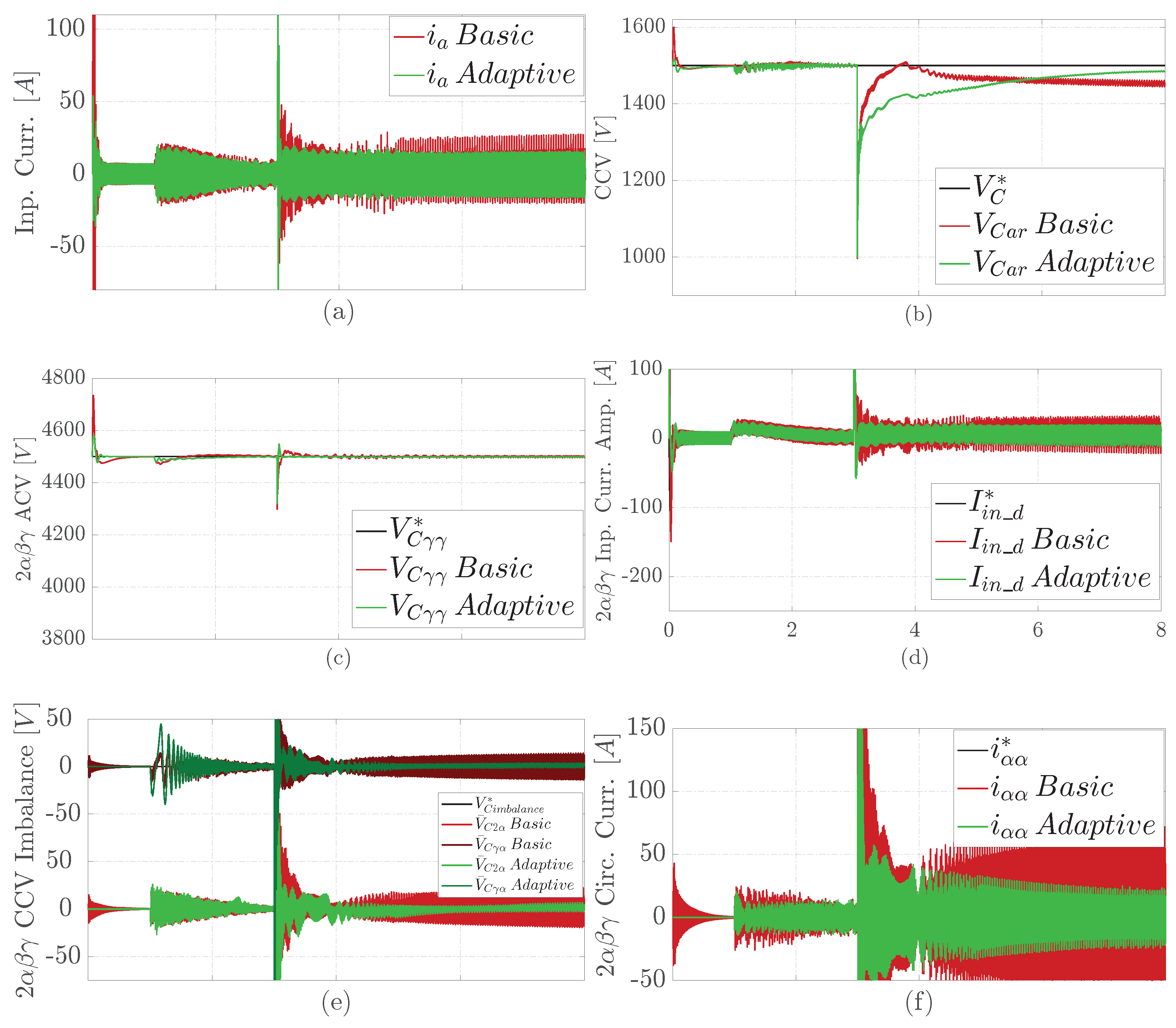
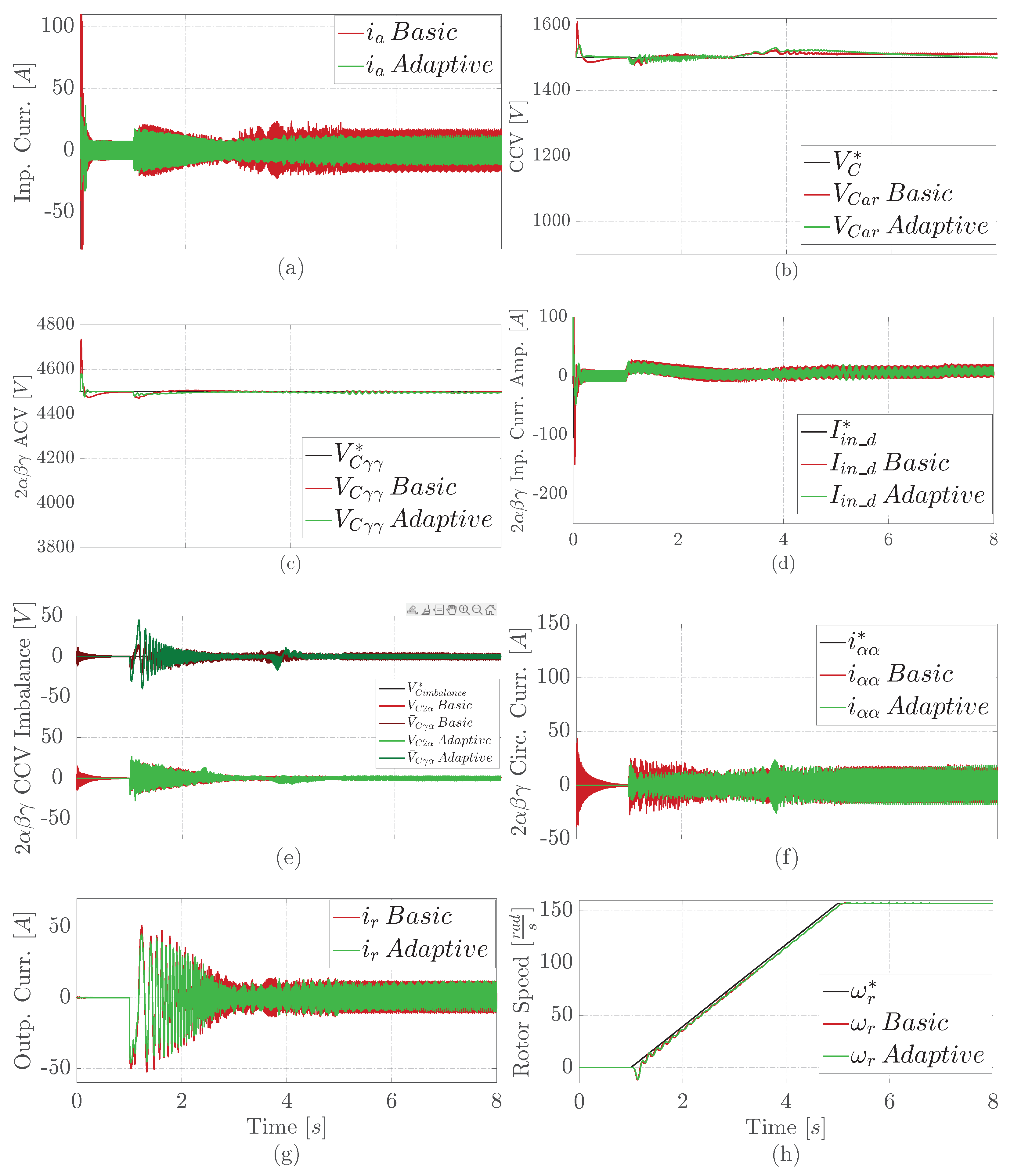
4.2. Results under a Normal Operation

Figure 3 shows the comparative simulation results under a normal operation. Here, we operate with the rated input and output voltages.

Figure 3a,g demonstrate that the M3C adaptive proposal results in $25\%$ lower input and output current consumption (with a reduction of 5 A) compared to the basis control that utilizes PI controllers. Moreover, the adaptive controllers also exhibit less input current overshoot than the PI controllers. Figure 3b shows that the proposed M3C adaptive control has $64\%$ less CCV overshoot (with a 70 V reduction) than the basic solution. Figure 3h shows that adaptive and basic solutions ensure that the rotor speed follows the reference.

Regarding the directly controlled variables in double-$\alpha \beta \gamma$ coordinates, both the adaptive and basic solution also follow the reference. However, the adaptive solution has lower overshoots of ACV in Figure 3c, input current amplitude in Figure 3d, intra and inter CCV imbalance in Figure 3e, and circulating current in Figure 3f. Moreover the adaptive proposal consumes less input and fewer circulation currents. As for the basic solution, the adaptive one has a 5 KHz noisy input amplitude in double-$\alpha \beta \gamma$.

4.3. Results under an Input Phase Imbalance

Figure 4 displays the comparative simulation results under an input phase imbalance. This first fault considers a drop of $10\%$ of the “a” phase voltage, starting at 3 s.

Figure 4a,g illustrate that, prior to the fault, the M3C adaptive proposal results in $25\%$ lower input and output current consumption, with a reduction of 5 A compared to the basis control. The adaptive controllers also show less input current overshoot than the PI controllers. However, during the first second after the fault, the basic solution deteriorated while the adaptive approach recovered its better performance faster. Figure 4b shows that the proposed M3C adaptive control has $64\%$ less CCV overshoot (with a 70 V reduction) than the basic solution, similar to Figure 3b. However, the basic solution deteriorated after the fault while the adaptive approach tended to recover its performance. Figure 4h demonstrates that both the proposal and basic M3C controllers maintain the rotor speed in line with the reference, similar to Figure 3d. This is evident even when a fault occurs at 3 s, as it does not affect the pumping speed response.

Regarding the variables in double-$\alpha \beta \gamma$ coordinates, again, the adaptive solution has lower overshoots of ACV in Figure 3c, input current amplitude in Figure 3d, intra and inter CCV imbalance in Figure 3e, and circulating current in Figure 3f. Moreover, the adaptive proposal consumes less input and circulation currents before the fault. After, the adaptive proposal completely recovers its performance within 2 s in contrast to the basic solution.

4.4. Results under a Cluster Cell Short Circuit

Figure 5 exhibits the comparative simulation results under a cluster cell short circuit. This fault happens in cell one of the cluster $ar$ at 3 s.

Figure 5a,g show that, prior to the fault, the M3C adaptive proposal results in $25\%$ lower input and output current consumption, with a reduction of 5 A compared to the basis control. However, during the first two seconds after the fault, the basic solution deteriorated and had a $70\%$ increase in input current consumption, increasing by 35 A compared to the adaptive approach. Figure 5b shows that the M3C adaptive control method has a $64\%$ reduction in CCV overshoot compared to the basic solution, reducing 70 V. This reduction is similar to the one shown in Figure 3b. However, the basic solution demonstrates a quicker CCV to recovery after the fault tending toward the CCV reference of 1500 V. Figure 5h demonstrates that both the proposal and basic M3C controllers maintain the rotor speed in line with the reference, similar to Figure 3d and Figure 4d. Again. this is observed even after the fault happens at 3 s, which does not have an impact on the pumping speed’s response.

Regarding the variables in double-$\alpha \beta \gamma$ coordinates, a similar behavior to the one shown in Figure 3 is obtained. The adaptive solution has lower overshoots of ACV in Figure 5c, input current amplitude in Figure 5d, intra and inter CCV imbalance in Figure 5e, and circulating current in Figure 5f. After the fault, the adaptive solution completely recovers its performance within 2 s, while the basic solution does not.

4.5. Results under an Opened Cluster Cell

Figure 6 exhibits the comparative simulation results under an opened cluster cell. This fault occurs in cell one of the cluster $ar$ at 3 s. Figure 6 describes a similar behavior to previously described faulty situations. However, both solutions have a lower degradation under this fault.

4.6. Results under Parameters Changes of the Motor–Pump Set

Figure 7 exhibits the comparative simulation results under one of the most probable faults in the pump-PMSM set. It starts with the short of the stator winding turns, provoking pumps’ mechanical difficulties. Specifically, there is a 0.8 times decrease in $R_s$, $L_d$, and $L_q$ at 5 s, and a 1.5 times increase in both $T_0$ and $K_{load}$ at 7 s.

Figure 7a,g show that, before the fault, the M3C adaptive proposal behaves similarly under a normal operation. It has 25% lower input and output current consumption, with a reduction of 5 A compared to the basis control. However, unlike the basic solution with a 3 A increase in input current consumption, the adaptive approach kept the input current consumption after the fault at 5 s. Compared to normal operation, there is a 4 A current consumption increase after the load torque rise at 7 s.

Figure 7b shows that the M3C adaptive control method has a 64% reduction in CCV overshoot compared to the basic solution, reducing 70 V. This reduction is similar to the one shown in Figure 3b. Moreover, unlike the PI controller’s basic solution, the proposal fully recovered its performance after the faults.

Figure 7h demonstrates that both the proposal and basic M3C controllers maintain the rotor speed in line with the reference, similar to Figure 3d. Again, this is observed even after the fault happens at 5 s and 7 s, which does not impact the pumping speed’s response.

Regarding the variables in double-$\alpha \beta \gamma$ coordinates, a similar behavior to the one shown in Figure 3 is obtained. The adaptive solution has lower overshoots of ACV in Figure 7c, input current amplitude in Figure 7d, intra and inter CCV imbalance in Figure 7e, and circulating current in Figure 7f. After the faults, the adaptive solution completely recovers its performance, while the basic solution does not.

Remark 6.

The M3C is a high-power converter that operates at a lower switching frequency than 10 Hz, resulting in a higher sampling time. Moreover, our strategy synthesizes the voltage references using PS-PWM, yielding a high-power quality even for lower frequencies [19,31]. However, the simulation tests were conducted at higher switching frequencies of 15 kHz (sampling time of 66.6 $\mu s)$ and 20 kHz (sampling time of 50 $\mu s$) to verify the computational burden. Both basic and proposed solutions ran correctly despite the worst scenario of a diminished sample time. Additionally, a technique with similar computational complexity to the proposal was successfully implemented at 10 kHz in [42]. Finally, proposal implementation could be improved further after analyzing different solver choices, simulation steps, and relative tolerance [43].

5. Conclusions

In this study, adaptive control for an M3C-based variable speed drive powering multiple PMSM-driven centrifugal pumps was proposed. The controller design considered this applifcation’s mathematical model, having unknown plant parameters, unknown disturbances, and unmodeled dynamics of the cell inverters that cause delays (please see Remark 4). As a result, the study found that the adaptive proposal offers better performance and fault tolerance than the non-adaptive solution based on PI controllers.

The first step was to obtain the multivariable M3C state-space model for control, which allowed for the design and implementation of novel MIMO adaptive controllers. Notably, the paper proposed and applied a novel cascade APBC-PBMRAC to the M3C. Simulation results demonstrate that the proposal and basic M3C controllers ensure that the rotor speed follows the reference, even when a fault occurs. However, the proposal has several advantages over the basic solution:

• It reduces the number of non-adaptive PI controllers from sixteen (16) to five (5) MIMO adaptive controllers.
• It is a more straightforward solution that does not require previous estimation of the plant parameters, reducing the commissioning time.
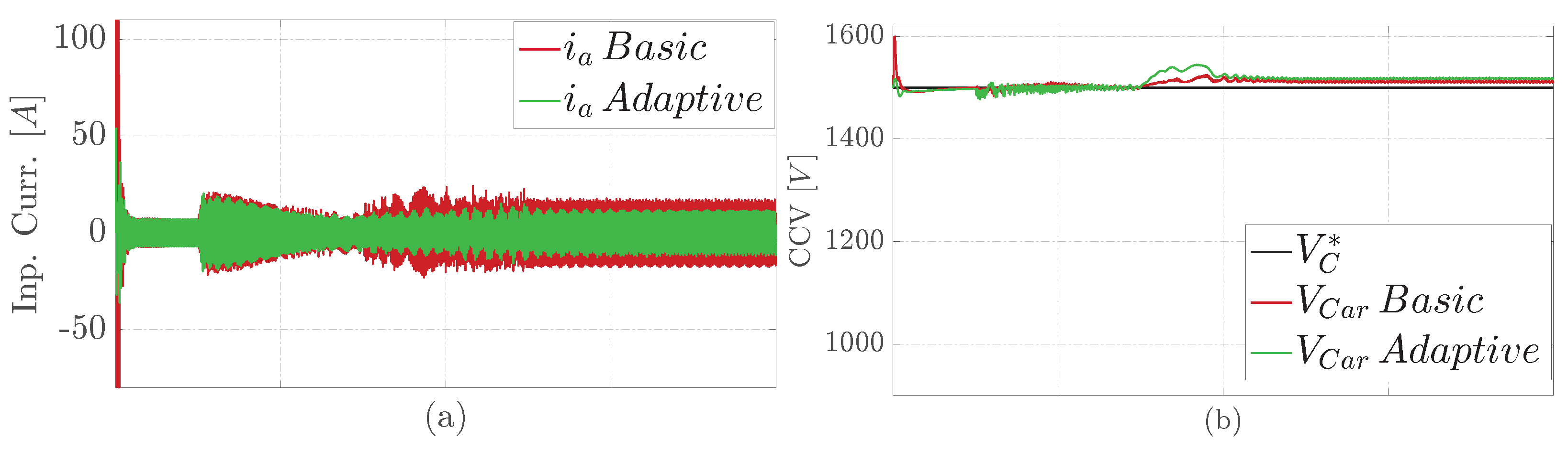
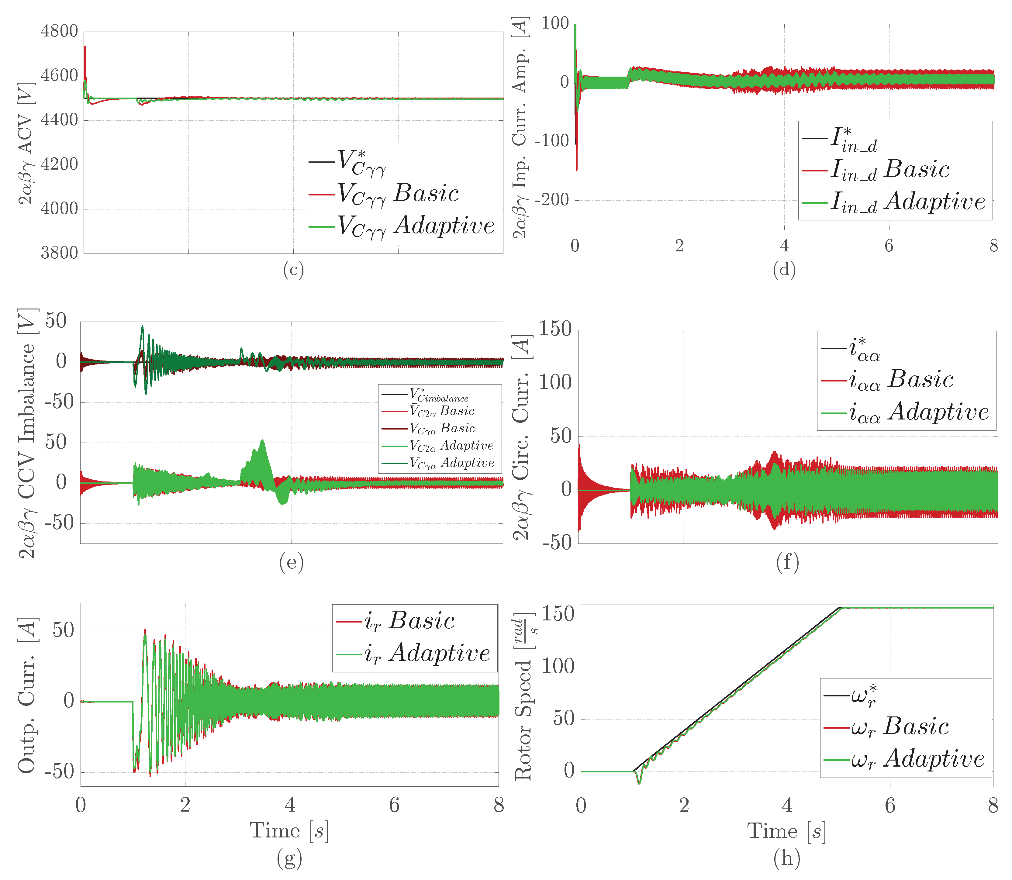
• The proposed adaptive control has fewer overshoots than the basic solution.
• Additionally, it shows a more stable CCV response (less noisy), which is as expected due to the APBC-PBMRAC design.
• Finally, the basic solution tends to remain degraded after a fault, while the adaptive approach tends to recover quickly from any studied fault.

References

1. Lin, Y.; Li, X.; Zhu, Z.; Wang, X.; Lin, T.; Cao, H. An energy consumption improvement method for centrifugal pump based on bionic optimization of blade trailing edge. Energy 2022, 246, 123323. [Google Scholar] [CrossRef]
2. Beck, M.; Sperlich, A.; Blank, R.; Meyer, E.; Binz, R.; Ernst, M. Increasing energy efficiency in water collection systems by submersible PMSM well pumps. Water 2018, 10, 1310. [Google Scholar] [CrossRef]
3. Candelo-Zuluaga, C.; Riba, J.R.; Espinosa, A.G.; Blanch, P.T. Customized PMSM design and optimization methodology for water pumping applications. IEEE Trans. Energy Convers. 2021, 37, 454–465. [Google Scholar] [CrossRef]
4. Hebala, A.; Nuzzo, S.; Connor, P.H.; Volpe, G.; Gerada, C.; Galea, M. Analysis and Mitigation of AC Losses in High Performance Propulsion Motors. Machines 2022, 10, 780. [Google Scholar] [CrossRef]
5. Kashif, M.; Singh, B. Reduced-Sensor-Based Multistage Model Reference Adaptive Control of PV-Fed PMSM Drive for Water Pump. IEEE Trans. Ind. Electron. 2022, 70, 3782–3792. [Google Scholar] [CrossRef]
6. Kashif, M.; Singh, B. Modified Active-Power MRAS Based Adaptive Control with Reduced Sensors for PMSM Operated Solar Water Pump. IEEE Trans. Energy Convers. 2022, 38, 38–52. [Google Scholar] [CrossRef]
7. Dini, P.; Saponara, S. Review on model based design of advanced control algorithms for cogging torque reduction in power drive systems. Energies 2022, 15, 8990. [Google Scholar] [CrossRef]
8. He, R.; Han, Q. Dynamics and stability of permanent-magnet synchronous motor. Math. Probl. Eng. 2017, 2017, 4923987. [Google Scholar] [CrossRef]
9. Annaswamy, A.M.; Narendra, K.S. Stable Adaptive Systems; Prentice Hall: Hoboken, NJ, USA, 1989. [Google Scholar]
10. Eugene, L.; Kevin, W.; Howe, D. Robust and Adaptive Control with Aerospace Applications; Springer: London, UK, 2013. [Google Scholar]
11. Travieso-Torres, J.C.; Duarte-Mermoud, M.A.; Estrada, J.L. Tracking control of cascade systems based on passivity: The non-adaptive and adaptive cases. ISA Trans. 2006, 45, 435–445. [Google Scholar] [CrossRef]
12. Travieso-Torres, J.C.; Ricaldi-Morales, A.; Véliz-Tejo, A.; Leiva-Silva, F. Robust Cascade MRAC for a Hybrid Grid-Connected Renewable Energy System. Processes 2023, 11, 1774. [Google Scholar] [CrossRef]
13. Gili, L.C.; Dias, J.C.; Lazzarin, T.B. Review, Challenges and Potential of AC/AC Matrix Converters CMC, MMMC, and M3C. Energies 2022, 15, 9421. [Google Scholar] [CrossRef]
14. Pires, V.F.; Cordeiro, A.; Foito, D.; Pires, A.J. Fault-tolerant multilevel converter to feed a switched reluctance machine. Machines 2022, 10, 35. [Google Scholar] [CrossRef]
15. Diaz, M.; Cardenas, R.; Ibaceta, E.; Mora, A.; Urrutia, M.; Espinoza, M.; Rojas, F.; Wheeler, P. An Overview of Modelling Techniques and Control Strategies for Modular Multilevel Matrix Converters. Energies 2020, 13, 4678. [Google Scholar] [CrossRef]
16. Kucka, J.; Karwatzki, D.; Mertens, A. AC/AC modular multilevel converters in wind energy applications: Design considerations. In Proceedings of the 2016 18th European Conference on Power Electronics and Applications (EPE’16 ECCE Europe), Karlsruhe, Germany, 5–9 September 2016; pp. 1–10. [Google Scholar]
17. Miura, Y.; Mizutani, T.; Ito, M.; Ise, T. Modular multilevel matrix converter for low frequency AC transmission. In Proceedings of the 2013 IEEE 10th International Conference on Power Electronics and Drive Systems (PEDS), Kitakyushu, Japan, 22–25 April 2013; pp. 1079–1084. [Google Scholar]
18. Bontemps, P.; Milovanovic, S.; Dujic, D. Performance analysis of energy balancing methods for matrix modular multilevel converters. IEEE Trans. Power Electron. 2022, 38, 2910–2924. [Google Scholar] [CrossRef]
19. Fan, B.; Wang, K.; Wheeler, P.; Gu, C.; Li, Y. An optimal full frequency control strategy for the modular multilevel matrix converter based on predictive control. IEEE Trans. Power Electron. 2017, 33, 6608–6621. [Google Scholar] [CrossRef]
20. Fan, B.; Wang, K.; Wheeler, P.; Gu, C.; Li, Y. A branch current reallocation based energy balancing strategy for the modular multilevel matrix converter operating around equal frequency. IEEE Trans. Power Electron. 2017, 33, 1105–1117. [Google Scholar] [CrossRef]
21. Kawamura, W.; Chen, K.L.; Hagiwara, M.; Akagi, H. A low-speed, high-torque motor drive using a modular multilevel cascade converter based on triple-star bridge cells (MMCC-TSBC). IEEE Trans. Ind. Appl. 2015, 51, 3965–3974. [Google Scholar] [CrossRef]
22. Wang, C.; Zheng, Z.; Wang, K.; Li, Y. Fault detection and tolerant control of IGBT open-circuit failures in modular multilevel matrix converters. IEEE J. Emerg. Sel. Top. Power Electron. 2022, 10, 6714–6727. [Google Scholar] [CrossRef]
23. Wang, C.; Zheng, Z.; Wang, K.; Yang, B.; Zhou, P.; Li, Y. Analysis and control of modular multilevel matrix converters under branch fault conditions. IEEE Trans. Power Electron. 2021, 37, 1682–1699. [Google Scholar] [CrossRef]
24. Wang, C.; Zheng, Z.; Wang, K.; Li, Y. Submodule Fault-Tolerant Control of Modular Multilevel Matrix Converters With Adaptive Optimum Common-Mode Voltage Injection. IEEE Trans. Power Electron. 2022, 37, 7548–7554. [Google Scholar] [CrossRef]
25. Guo, F.; Yu, J.; Ni, Q.; Zhang, Z.; Meng, J.; Wang, Y. Grid-forming control strategy for PMSG wind turbines connected to the low-frequency AC transmission system. Energy Rep. 2023, 9, 1464–1472. [Google Scholar] [CrossRef]
26. Kawamura, W.; Hagiwara, M.; Akagi, H. Control and experiment of a modular multilevel cascade converter based on triple-star bridge cells. IEEE Trans. Ind. Appl. 2014, 50, 3536–3548. [Google Scholar] [CrossRef]
27. Erickson, R.W.; Al-Naseem, O.A. A new family of matrix converters. In Proceedings of the IECON’01. 27th Annual Conference of the IEEE Industrial Electronics Society (Cat. No.37243), Denver, CO, USA, 29 November–2 December 2001; Volume 2, pp. 1515–1520. [Google Scholar]
28. Zhang, Z.; Jin, Y.; Xu, Z. Modeling and Control of Modular Multilevel Matrix Converter for Low-Frequency AC Transmission. Energies 2023, 16, 3474. [Google Scholar] [CrossRef]
29. Bravo, P.; Pereda, J.; Merlin, M.M.; Neira, S.; Green, T.C.; Rojas, F. Modular Multilevel Matrix Converter as Solid State Transformer for Medium and High Voltage AC Substations. IEEE Trans. Power Deliv. 2022, 37, 5033–5043. [Google Scholar] [CrossRef]
30. Park, R.H. Two-reaction theory of synchronous machines generalized method of analysis-part I. Trans. Am. Inst. Electr. Eng. 1929, 48, 716–727. [Google Scholar] [CrossRef]
31. Kammerer, F.; Gommeringer, M.; Kolb, J.; Braun, M. Energy balancing of the modular multilevel matrix converter based on a new transformed arm power analysis. In Proceedings of the 2014 IEEE 16th European Conference on Power Electronics and Applications, Lappeenranta, Finland, 26–28 August 2014; pp. 1–10. [Google Scholar]
32. Kawamura, W.; Chiba, Y.; Akagi, H. A broad range of speed control of a permanent magnet synchronous motor driven by a modular multilevel TSBC converter. IEEE Trans. Ind. Appl. 2017, 53, 3821–3830. [Google Scholar] [CrossRef]
33. Kawamura, W.; Hagiwara, M.; Akagi, H.; Tsukakoshi, M.; Nakamura, R.; Kodama, S. AC-Inductors design for a modular multilevel TSBC converter, and performance of a low-speed high-torque motor drive using the converter. IEEE Trans. Ind. Appl. 2017, 53, 4718–4729. [Google Scholar] [CrossRef]
34. Arias-Esquivel, Y.; Cardenas, R.; Urrutia, M.; Diaz, M.; Tarisciotti, L.; Clare, J.C. Continuous control set model predictive control of a modular multilevel converter for drive applications. IEEE Trans. Ind. Electron. 2022, 70, 8723–8733. [Google Scholar] [CrossRef]
35. Travieso-Torres, J.C.; Vilaragut-Llanes, M.; Costa-Montiel, Á.; Duarte-Mermoud, M.A.; Aguila-Camacho, N.; Contreras-Jara, C.; Álvarez-Gracia, A. New adaptive high starting torque scalar control scheme for induction motors based on passivity. Energies 2020, 13, 1276. [Google Scholar] [CrossRef]
36. Ogata, K. Modern Control Engineering; Prentice Hall: Upper Saddle River, NJ, USA, 2010; Volume 5. [Google Scholar]
37. Diaz, M.; Cardenas, R.; Espinoza, M.; Hackl, C.M.; Rojas, F.; Clare, J.C.; Wheeler, P. Vector control of a modular multilevel matrix converter operating over the full output-frequency range. IEEE Trans. Ind. Electron. 2018, 66, 5102–5114. [Google Scholar] [CrossRef]
38. Véliz-Tejo, A.; Travieso-Torres, J.C.; Peters, A.A.; Mora, A.; Leiva-Silva, F. Normalized-Model Reference System for Parameter Estimation of Induction Motors. Energies 2022, 15, 4542. [Google Scholar] [CrossRef]
39. O’Rourke, C.J.; Qasim, M.M.; Overlin, M.R.; Kirtley, J.L. A geometric interpretation of reference frames and transformations: dq0, clarke, and park. IEEE Trans. Energy Convers. 2019, 34, 2070–2083. [Google Scholar] [CrossRef]
40. Clarke, E. Circuit Analysis of AC Power Systems: Symmetrical and Related Components; Wiley: Hoboken, NJ, USA, 1943; Volume 1. [Google Scholar]
41. Maity, A.; Höcht, L.; Holzapfel, F. Time-varying parameter model reference adaptive control and its application to aircraft. Eur. J. Control 2019, 50, 161–175. [Google Scholar] [CrossRef]
42. Arias-Esquivel, Y.; Cárdenas, R.; Tarisciotti, L.; Díaz, M.; Mora, A. A Two-Step Continuous-Control-Set MPC for Modular Multilevel Converters Operating with Variable Output Voltage and Frequency. IEEE Trans. Power Electron. 2023, 1–12. [Google Scholar] [CrossRef]
43. Dini, P.; Ariaudo, G.; Botto, G.; Greca, F.L.; Saponara, S. Real-time electro-thermal modelling & predictive control design of resonant power converter in full electric vehicle applications. IET Power Electron. 2023. [Google Scholar] [CrossRef]
Figure 1. Basic power topology of an M3C for transferring energy between the power supply and the load, which is based on [15,18,25,26].
Machines 11 00884 g001
Figure 3. Comparative simulation results under normal operation: (a) phase a input current, (b) branch a r CCV, (c) controlled 2 α β γ ACV, (d) controlled d component of the input current amplitude in 2 α β γ , (e) controlled intra and inter CCV imbalance in 2 α β γ , (f) controlled α α component of the circulating current in 2 α β γ , (g) phase r output current, (h) PMSM angular rotor speed.
Machines 11 00884 g003
Figure 4. Comparative simulation results under an input voltage imbalance, with a 10 % voltage drop in phase a at 3 s: (a) phase a input current, (b) branch a r CCV, (c) controlled 2 α β γ ACV, (d) controlled d component of the input current amplitude in 2 α β γ , (e) controlled intra and inter CCV imbalance in 2 α β γ , (f) controlled α α component of the circulating current in 2 α β γ , (g) phase r output current, (h) PMSM angular rotor speed.
Machines 11 00884 g004
Figure 5. Comparative simulation results under a cluster a r short circuit at 3 s: (a) phase a input current, (b) branch a r CCV, (c) controlled 2 α β γ ACV, (d) controlled d component of the input current amplitude in 2 α β γ , (e) controlled intra and inter CCV imbalance in 2 α β γ , (f) controlled α α component of the circulating current in 2 α β γ , (g) phase r output current, (h) angular rotor speed.
Machines 11 00884 g005aMachines 11 00884 g005b
Figure 6. Comparative simulation results under a cluster a r open circuit at 3 s: (a) phase a input current, (b) branch a r CCV, (c) controlled 2 α β γ ACV, (d) controlled d component of the input current amplitude in 2 α β γ , (e) controlled intra and inter CCV imbalance in 2 α β γ , (f) controlled α α component of the circulating current in 2 α β γ , (g) phase r output current, (h) PMSM angular rotor speed.
Machines 11 00884 g006aMachines 11 00884 g006b
Figure 7. Comparative simulation results under parameters changes of the motor at 5 s (there is 0.8 times decrease in R s , L d , and L q ), and the pump at 7 s (there is a 1.5 times increase in both T 0 and K l o a d ): (a) phase a input current, (b) branch a r CCV, (c) controlled 2 α β γ ACV, (d) controlled d component of the input current amplitude in 2 α β γ , (e) controlled intra and inter CCV imbalance in 2 α β γ , (f) controlled α α component of the circulating current in 2 α β γ , (g) phase r output current, (h) PMSM angular rotor speed.
Machines 11 00884 g007