Abstract
Nowadays, collaborative operations between Remotely Operated Vehicles (ROVs) face considerable challenges, particularly in leader–follower schemes. The underwater environment imposes limitations on acoustic modems, leading to reduced transmission speeds and increased latency in ROV position and speed transmission. This complicates effective communication between the ROVs. Traditional methods, such as Recursive Least Squares (RLS) predictors and the Kalman filter, have been employed to address these issues. However, these approaches have limitations in handling non-linear patterns and disturbances in underwater environments. This paper introduces a Convolutional Long Short-Term Memory (ConvLSTM) predictor designed to enhance communication and trajectory tracking between ROVs in a leader–follower scheme. The proposed ConvLSTM aims to address the shortcomings of previous methods by adapting effectively to varying conditions, including ocean currents, communication delays, and signal interruptions. Simulations were conducted to evaluate ConvLSTM’s performance and compare it with other advanced predictors, such as Multilayer Perceptron (MLP) and Long Short-Term Memory (LSTM), under different conditions. The results demonstrated that ConvLSTM achieved a 13.9% improvement in trajectory tracking, surpassing other predictors in scenarios that replicate real underwater conditions and multi-vehicle communication. These results highlight ConvLSTM’s potential to significantly enhance the performance and stability of collaborative ROV operations in dynamic underwater environments.
1. Introduction
Collaboration between Remotely Operated Vehicles (ROVs) in underwater activities is extremely advantageous and diverse. By permitting the simultaneous execution of multiple tasks instead of relying exclusively on a single vehicle, a significant improvement in operational efficiency is achieved and the total available cargo capacity is expanded. Moreover, coordinating the movements of multiple ROVs for the inspection of marine environments not only expands the work area but also reduces costs and facilitates more effective adaptation to changes, bringing greater flexibility and efficiency to underwater operations. An important additional advantage is the redundancy provided by the presence of multiple vehicles, which increases operational reliability by providing an alternative in the event of failure of one of the vehicles.
As a direct consequence of these operational advantages, a decrease in operating costs can be observed, as well as a notable increase in the speed and efficiency of underwater activities. Nowadays, a variety of collaborative tasks are available that use various control systems, the most notable being those that mention control challenges in a non-linear manner. Since the six-degree-of-freedom (DOF) dynamics of the system are highly non-linear and therefore difficult to control, innovative approaches have been developed to address this challenge.
In recent research, various technologies have been explored to address collaborative tasks in underwater environments. For example, some studies have chosen to use cameras for object detection, combining them with PID control systems and Kalman filters for this purpose [1]. Other researchers have found the use of acoustic modems in conjunction with non-linear control systems based on sliding modes [2] and have integrated these technologies with cameras to improve localization accuracy. Additionally, the potential of predictive control has been explored, especially when combined with acoustic modems to achieve greater control accuracy and efficiency [3]. On the other hand, backstepping control has also been proposed as an alternative to this type of problem [4].
The previous studies have overlooked communication constraints common in maritime environments, such as delays in data transmission, long sampling periods generated by sensors, and the inherent latency of acoustic modems. Furthermore, these studies have minimized the impacts of changes in the direction and strength of ocean currents. To address these challenges, the use of predictors has been used. These efforts can be divided into two main categories: classical predictors and intelligent predictors. Within the field of classical predictors, methods such as prediction using autoregressive models [5] are included, which have shown good results in situations such as the formation of ships with communication delays [6]. The combination of these approaches and predictive control techniques is proposed as a solution to optimize results during training [7]; this approach has also been used to mitigate chattering induced by communication delay, which has previously been successfully employed to improve the precision in the movement of a robotic arm [8]. The Kalman filter stands out as one of the most used approaches in this regard. These techniques have proven to be effective thanks to their extensive documentation and consistent results. However, it is essential to explore new strategies to improve prediction accuracy in marine environments, especially given the difficulty of variables and variable conditions of the underwater environment.
Advanced predictors are systems that incorporate membership functions and merge them with control techniques. This approach is used to make accurate estimates of the position of an ROV [9], considering the influence of ocean currents. Another notable area is recursive neural networks (RNNs), which excel at handling non-linear relationships and more complex patterns. This capability permits them to compensate for long frequency delays and periods, as well as predict patterns in waves and ocean currents. In this sense, promising results have been observed with techniques such as the modified neural network (ECRNet) to predict the slip caused by currents and improve the precision of the trajectory due to the noise generated by a GPS sensor and where memory is already implemented in the predictor. Likewise, the use of a Gated Recurrent Unit (GRU) [10] has shown good results, as has the application of RNN systems to improve the precision in the position of a glider. Among the most used techniques for their memory capacities are LSTM (Long Short-Term Memory) and its variants. They have been applied to analyze ocean currents and adjust PID control parameters accordingly. This methodology not only facilitates the understanding of ocean current dynamics but also allows optimization of PID control performance to maintain more accuracy and stable navigation in variable and challenging maritime environments. Integrating these current studies with dynamic adjustments of PID control represents an effective strategy to improve the adaptability and efficiency of underwater navigation systems [11], as well as in the present prediction to optimize neuro-PID (Proportional, Integral, Derivative) control [12]. Moreover, a technique called LSTM-Decay has emerged that is widely recognized for its ability to predict time delay and data loss, frequent phenomena due to effective communication between various sensors. This variant of recurrent neural networks has been highlighted for its ability to manage and mitigate the adverse effects of irregular communication between sensors, thus providing a significant improvement in the reliability and accuracy of the prediction of critical data [13]. This approach has been collaboratively implemented to determine a diver’s location and coordinate with an underwater vehicle. The integration of both systems allows effective and accurate synchronization between the activities of the diver and the operations of the underwater vehicle [14]. On the other hand, BiLSTM (Bidirectional and Unidirectional LSTM) has proven to be useful in compensating for the slipping caused by an acoustic GPS (Global Positioning System) [15]. In another paper, it was shown through experiments that the proposed model improved the prediction accuracy in terms of longitude, latitude, and altitude. These results show the effectiveness and reliability of the developed model to estimate geographic coordinates and altitude more accurately, providing a robust and reliable tool for applications that require precise and consistent localization [16]. In certain studies, Fuzzy control incorporating membership functions has been used to estimate both the sampling period and disturbances. This integration harnesses the adaptability of Fuzzy logic to handle uncertainties and varying conditions, allowing for robust estimation of key parameters essential for system stability and performance. By leveraging membership functions within Fuzzy control frameworks, researchers aim to enhance the accuracy and resilience of sampling period estimation, while also effectively leasing disturbances that could impact system behavior. This approach underestimates the versatility of Fuzzy control in addressing complex challenges in control and calculation within diverse technological applications [17]. From the literature reviewed, it is inferred that classical predictors have been used in collaborative tasks with delays, but without considering complications in sensor sampling periods. At the same time, intelligent predictors that have dealt with communication delays in addition to current changes have not considered vehicle collaboration. Therefore, this work focuses on proposing a ConvLSTM network, simulating the communication latency caused by acoustic modems, sensor sampling periods, and variant current changes, to obtain trajectory tracking in a leader tracker scheme.
The rest of the article is structured as follows: Section 2 shows the dynamics and hydrodynamics of autonomous underwater vehicles. Section 3 talks about the concept of leader–follower and how these vehicles can coordinate as a team. The control and its relationship with the positioning movement, the functionality and application of the simulation, and the results obtained are shown in Section 4, and finally, the conclusions derived from the study are presented in Section 5.
2. Materials and Methods
2.1. Kinematics and Hydrodynamics of Autonomous Underwater Vehicles
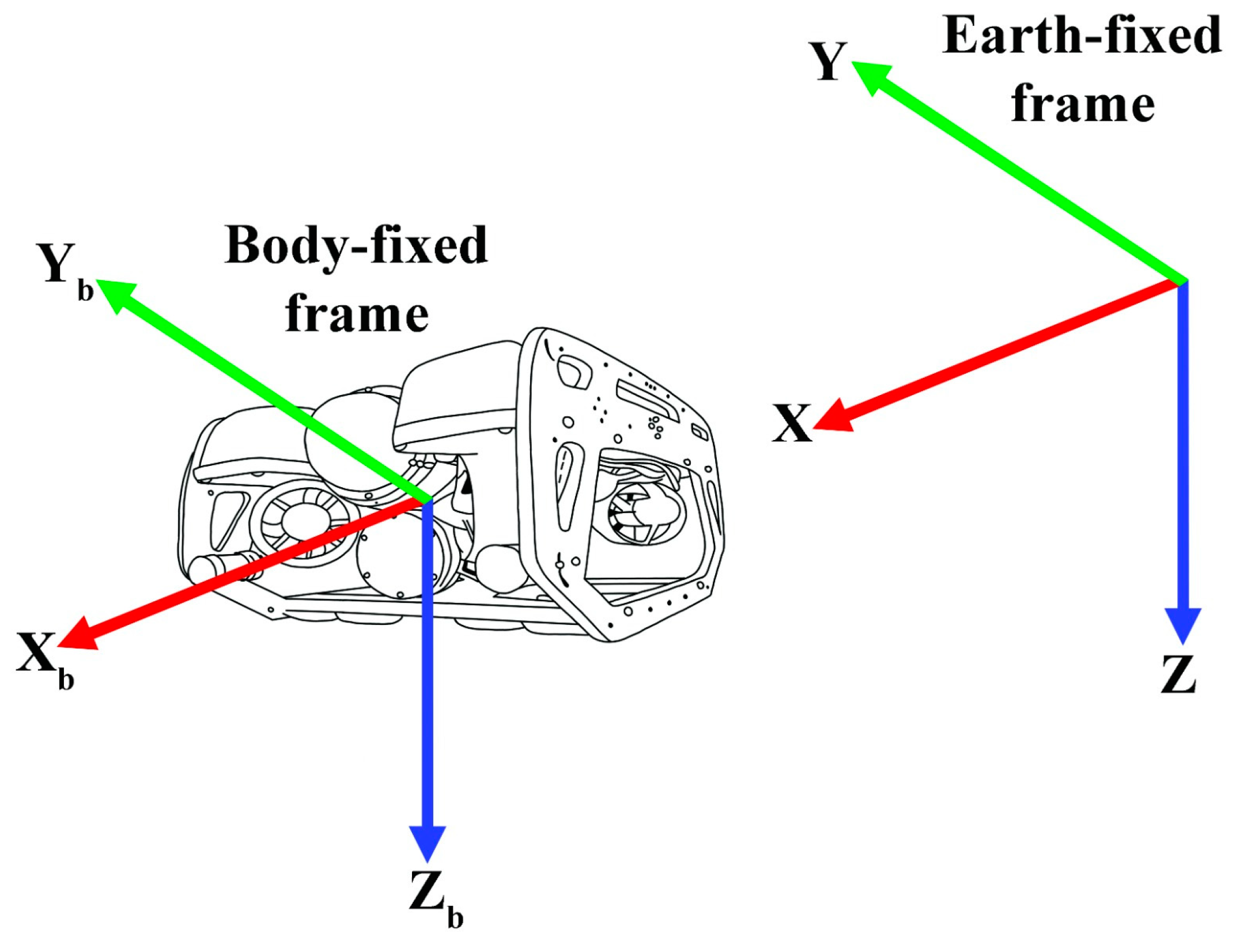
Fossen [18] details the main reference planes for the construction of the mathematical model of an underwater vehicle. One of these reference frames is the one fixed to the Earth (Earth-fixed frame), while the other is relative to the vehicle-body-fixed frame. Both frames present orthogonal axes, denoted as X, Y and Z, to refer, respectively, to the Earth-fixed frame plane and the body-fixed frame plane . These concepts are visually illustrated in Figure 1 and notation is shown in Table 1.
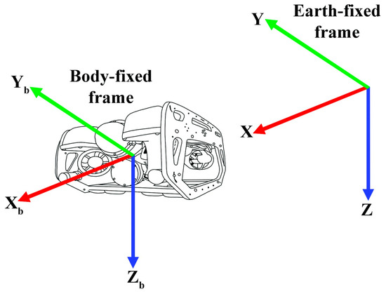
Figure 1.
Reference frame and axes of ROV2.

Table 1.
Notation of movements, name, position, velocity, force, and moments.
The location and speeds of the vehicle related to the body-fixed frame can be expressed as follows:
The forces and moments of the vehicle in the body-fixed frame can be expressed as
2.2. Hydrodynamic Model
The hydrodynamic model formulation of the ROV can be represented by the Newton–Euler Equation [18]:
where
- is the inertial and added mass matrix;
- is the rigid body and added mass centripetal and Coriolis matrix;
- is the hydrodynamic damping matrix;
- is the restitution force vector;
- is the thruster allocation matrix;
- is a vector containing the force generated by the thrusters;
- represents environmental disturbances.
2.3. Leader–Follower Scheme
Inside the scope of this research, the leader–follower method will be applied with the objective of facilitating coordinated collaboration between multiple factors. This strategy will make it possible to monitor and control various parameters, including distance both in the horizontal plane and in the depth dimension. Additionally, angles in the XY plane and Z plane will be handled, adding an extra level of precision and flexibility to the control process. As part of our methodology, a coordination relationship will initially be established in the two-dimensional plane, and we will then expand and apply these techniques in three-dimensional space. The use of drones has been taken as a reference and this concept is being applied to the development of underwater vehicles [19]. In vector analysis, position is defined by the following equation [19]:
while speed is expressed as
where
- the position of the leader in relation to the reference plane ;
- the desired distance between the leader and follower;
- the position of the follower with respect to the leader ;
- the speed of the leader in relation to the reference plane ;
- the desired speed between the leader and follower;
- follower speed .
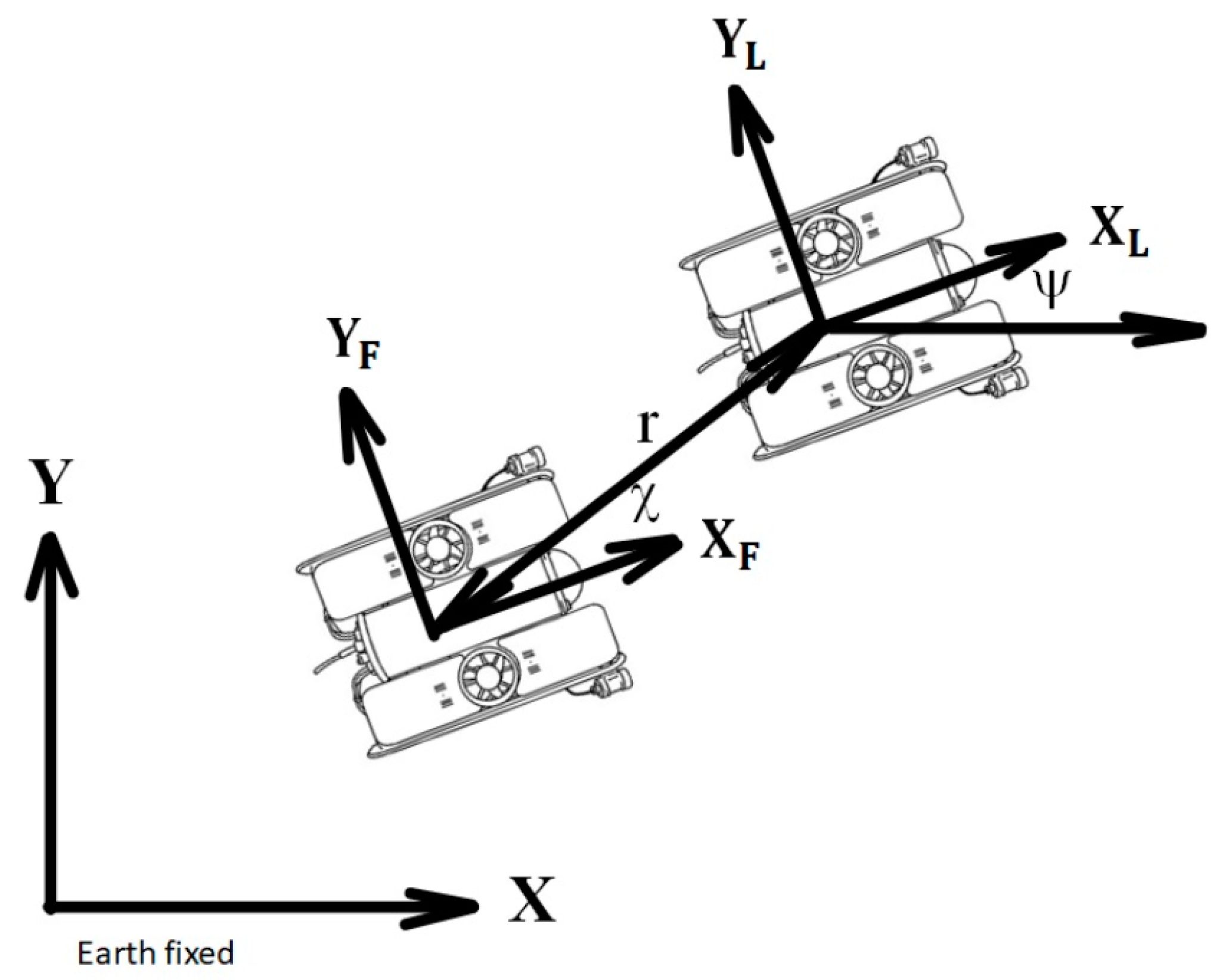
After carrying out a kinematic analysis (Figure 2) and focusing exclusively on the specific case presented in the plan, we have the following components: = 0.

Figure 2.
Vector relationship between the follower and the leader ROV in the XY plane.
Analyzing X:
Analyzing Y:
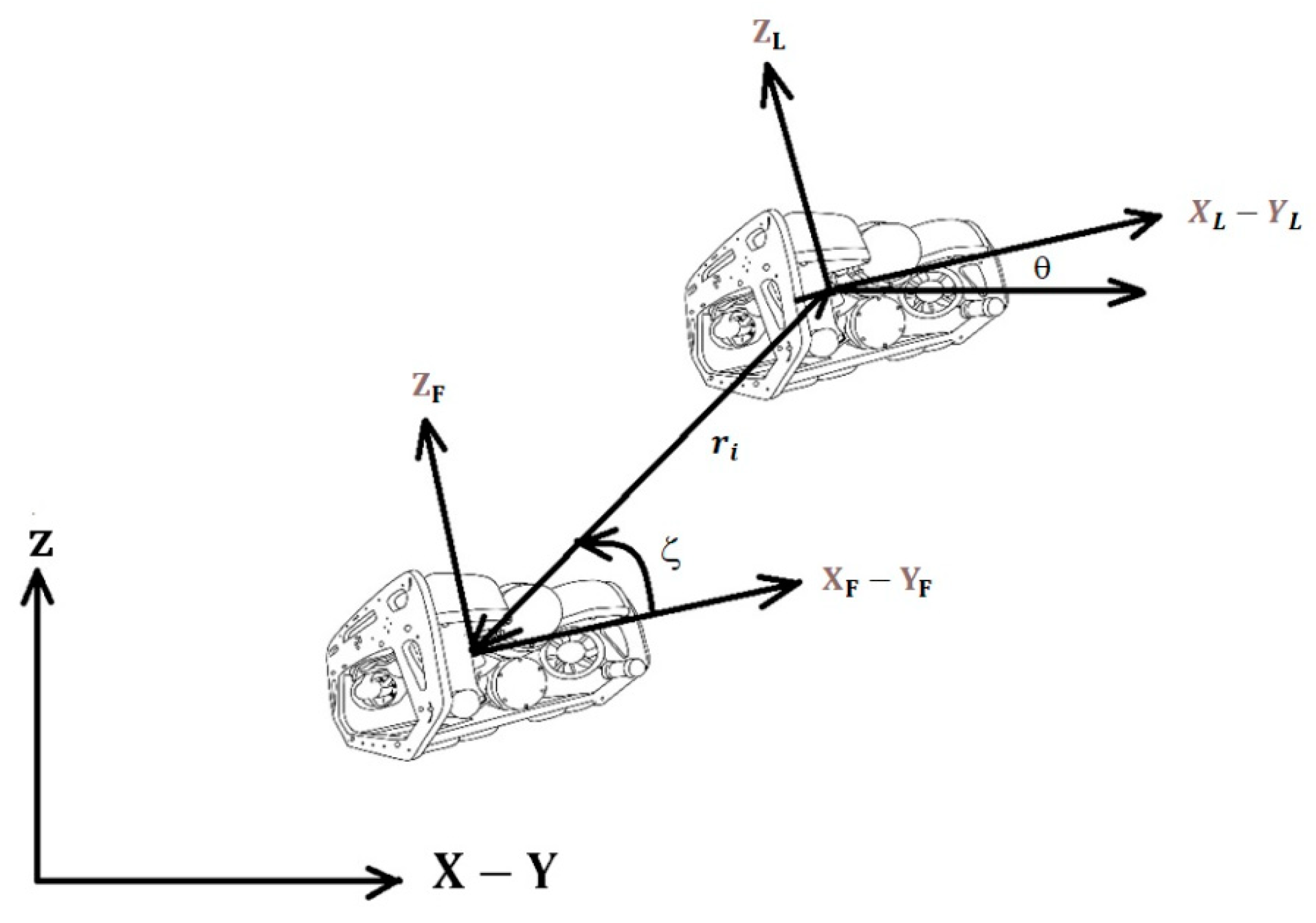
By conducting an analysis to manage the distance in space (Figure 3) and performing the relevant operations, the following equations are obtained below [19]:
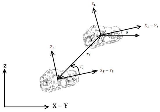
Figure 3.
Vector relationship between the follower and the leader ROV in space.
Because the leader will only experience changes in the angle ψ, the other angles can be considered zero. Therefore, the simplification of Equations (8)–(10) be as follows:
Now, substituting Equations (8)–(10) in Equation (4), the following is obtained:
These equations represent the desired positions concerning the position of the leader and the previously defined angle to obtain the desired speeds; Equations (16)–(18) are derived concerning time, and the following speed equations are obtained:
2.4. Scalable to n-Robots
There are various collaboration strategies between robots, with the leader–follower system being the focus. The theory of follower leadership, explored in the study [19], has been subject to adaptations, adjustments, and modifications in terms of its adaptation to application in underwater vehicles, guaranteeing that it does not interfere with the previously defined variables. To express this challenge more effectively, the following assumptions are introduced:
- i.
- Follower robots maintain predefined distances and angles from the leader.
- ii.
- The interaction between the follower robots is not considered.
- iii.
- It is ensured that the distances between the robots are wide enough to avoid collisions.
These restrictions facilitate the expression and application of the previously established equations to any number of robots in the system. The position equations are defined as follows:
represent the desired positions with respect to the leader of the n-follower, with respect to the leader, while , are the angles with respect to the leader.
To express the velocities of the n-follower, we proceed to derive (22), (23), and (24).
2.5. Controller
Although this work proposes a ConvLSTM predictor to address communication issues in leader–follower collaborative schemes for ROVs, a control law is still required to achieve the desired vehicle trajectories. Therefore, the control law from [20], which has proven effective for trajectory control, will be applied, as described in Equation (28). The stability of this control law has been rigorously tested and validated in [21,22].
where the term represents the position tracking error, with being the desired positions. In addition, is a positive diagonal gain matrix defined by dimension n × n, and α is a gain to be specified, with α > 0. The function sign(x) corresponds to the sign function, which is applied input by input to the vector x and
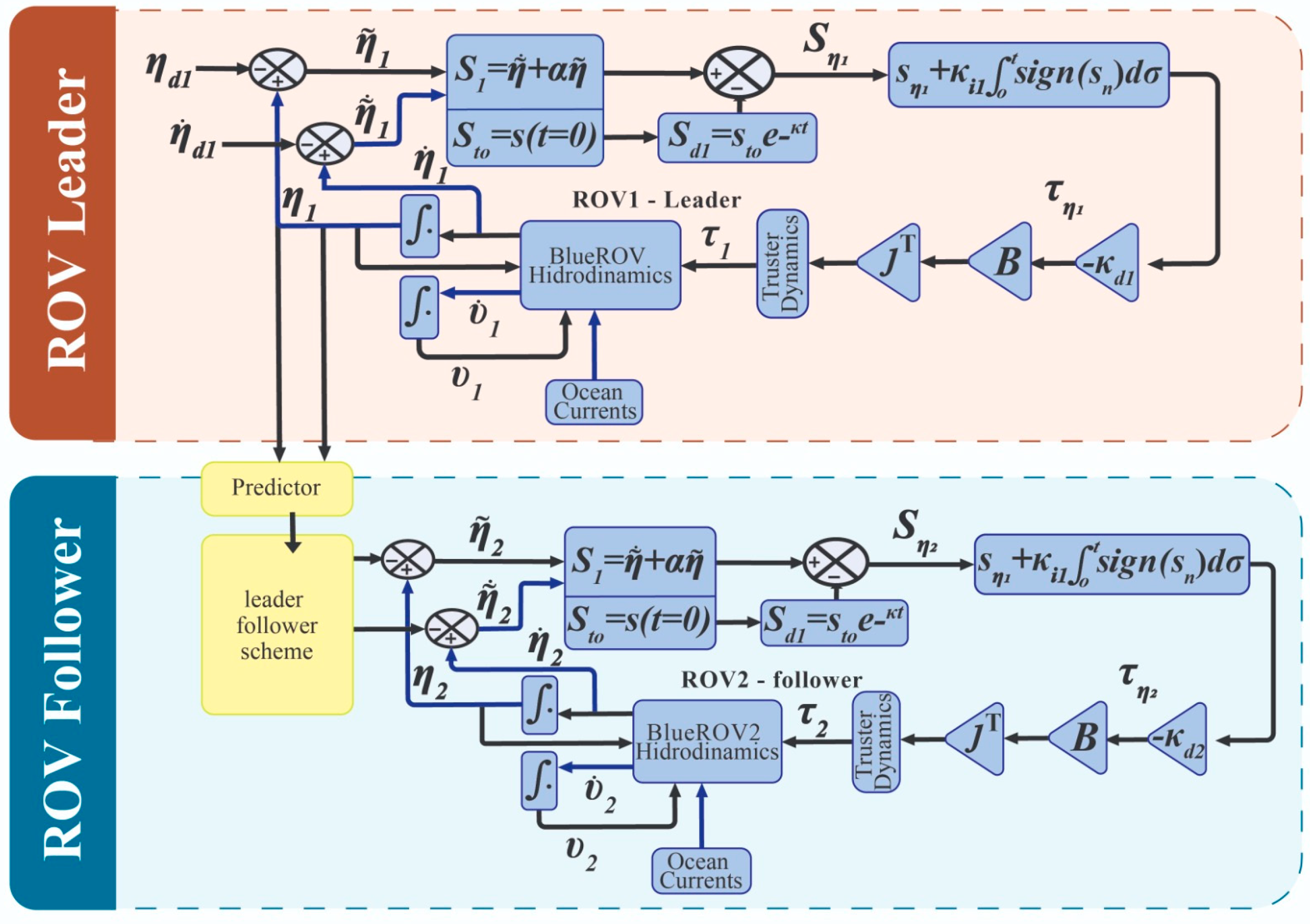
Figure 4 shows a diagram illustrating the communication between two vehicles and the control system. In the leader vehicle section of the diagram (light red), the leader vehicle receives the desired trajectory; it enters the control law to follow the desired trajectory. The current position of the leader vehicle is sent to the follower vehicle, which ensures that, regardless of the error in the leader’s trajectory, the follower will try to maintain the same desired position of the leader. In the section of the follower vehicle diagram (light blue), the information obtained from the sonar (leader position and angles) is first received by the predictor. This predictor forecasts the future positions and angles as well as recursively adjusting itself. The predicted data are then transmitted to the leader–follower scheme, and the desired trajectory is calculated from (3) to (18), allowing the follower to maintain its position relative to the leader. The variables and the control system are summarized in Table 2, detailing the parameters used to ensure the stability and efficiency of the control system.

Figure 4.
Law of control [20] and leader–follower schema.
Table 2.
Control variables.
2.6. Types of Predictors
A predictor, in control and dynamic systems, is an algorithm that estimates the future behavior of a system or process based on its current state and known inputs. It takes the currently available information to adjust and predict the evolution of the system. Predictors are based on mathematical models, machine learning techniques, or statistical approaches, among other methods. Their main function is to estimate values to make decisions or adjustments in real time. In applications with ROVs (Remotely Operated Vehicles), a predictor can be used to predict the future position of the vehicle to plan and execute efficient and safe movements.
The predictors used in this article are as follows:
- I.
- Recursive least squares with forgetting;
- II.
- Kalman filter;
- III.
- MLP (Multilayer Perceptron);
- IV.
- LSTM (Long Short-Term Memory);
- V.
- Convolutional LSTM (ConvLSTM).
I. Recursive least squares (RLS) is a parameter estimation method used in signal processing, control, and artificial intelligence. RLS estimates the parameters of a mathematical model from a set of observations or measurements by minimizing the mean square error between the actual observations and the model predictions. The main advantage is its recursive nature; i.e., the estimation of the model parameters is continuously updated as new observations are received, rather than estimating all parameters at once. This makes it especially useful for real-time applications, where data are received continuously and a real-time estimation of the model parameters is needed [23]. In marine communications, it has been used to compensate for the delay in acoustic modem communications between two static devices [5].
II. The Kalman filter is an estimation algorithm used to predict the state of a dynamical system from a series of noisy measurements. It was developed by mathematician and statistician Rudolf Kalman in the 1960s and is a fundamental tool in a wide range of fields, including engineering, navigation, robotics, economics, and more. The Kalman filter makes real-time estimates by computing based on recent measurements and previous estimates of the system state. It works in two main phases: prediction and update [24]. In underwater robotics, it is used to compensate for communication delays [1].
Recursive neural networks on time series are an approach to modeling and predicting sequential data that have a temporal structure. Unlike other time series models, such as autoregressive models or recurrent neural networks (RNNs), recursive neural networks address the recursive nature of time series, where future values depend on past and present values, but also, they may depend on more complex and non-linear relationships within the time series. Those handled in this paper are MLP (Multilayer Perceptron), LSTM (Long Short-Term Memory), ConvLSTM (Convolutional Long Short-Term Memory).
III. MLP (Multilayer Perceptron) is a type of artificial neural network architecture in which multiple layers of nodes (neurons) are connected in a feedback structure. Each neuron in a layer is connected to all neurons in the next layer, with no recurrent connections, meaning that information flows in one direction, from input to output. When applied to time series, MLPs can model complex relationships between input features and desired outputs as a function of time and add connections between different layers [25]. Its main use is to estimate the positions of underwater vehicles with sea currents [9]. The basic structure is shown in Figure 5.
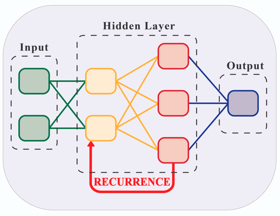
Figure 5.
MLP basic structure.
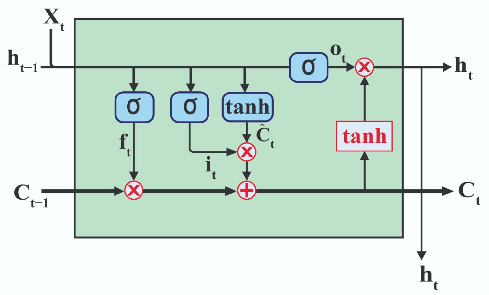
IV. LSTM, which stands for Long Short-Term Memory, is a type of recurrent neural network (RNN) architecture designed to mention the disappearing gradient problem that occurs in traditional RNNs. The disappearing gradient problem refers to the problem where gradients (derivatives used in training) decrease as they propagate backward in time during training, which can lead to difficulties in learning long-range dependencies. LSTM networks address this problem by introducing a more complicated memory cell structure composed of multiple gates. These gates regulate the flow of information within the cell, allowing the LSTM to selectively remember or forget information over time [26]. It has been used to optimize a PID with current changes [11]. The basic structure is shown in image Figure 6.
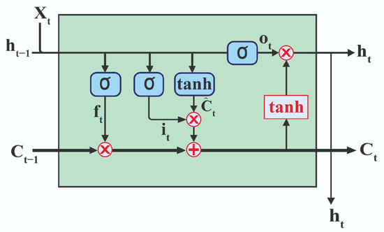
Figure 6.
LSTM basic structure.
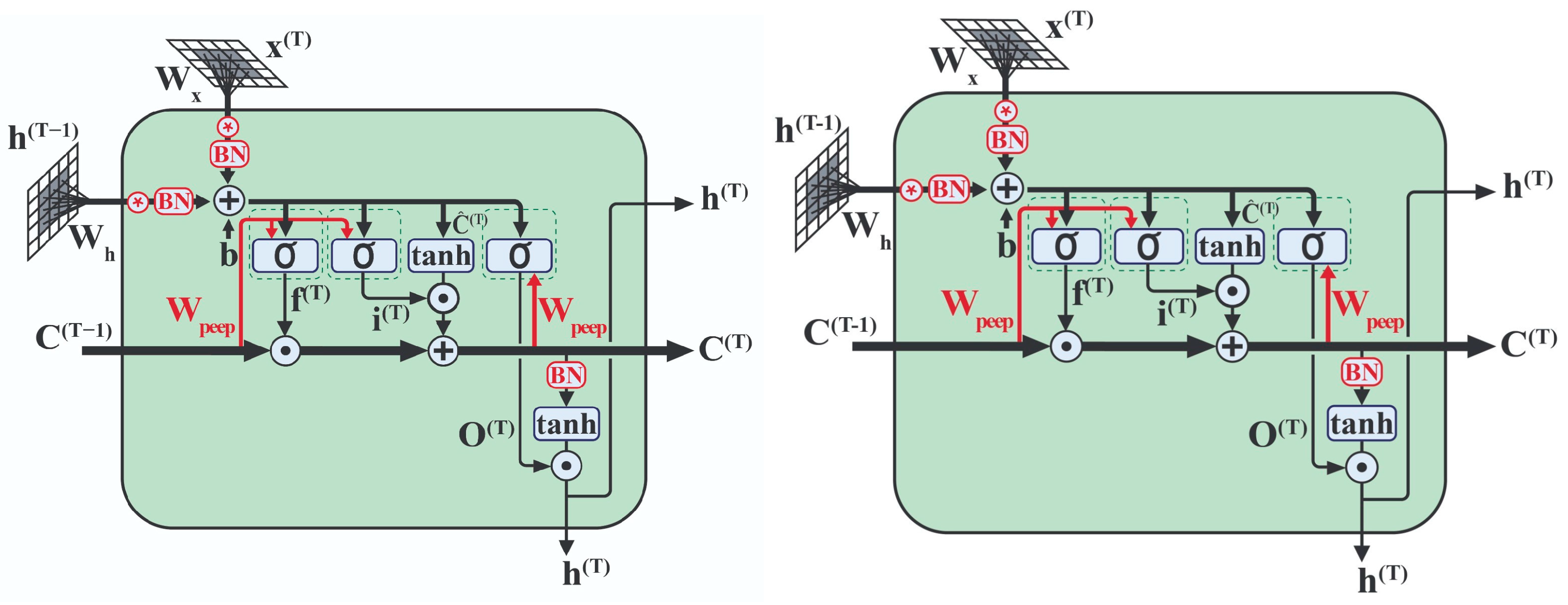
V. Convolutional LSTM (ConvLSTM) is a variant of recurrent neural networks (RNNs) that combines the properties of LSTM (Long Short-Term Memory) layers with convolution operations, permitting both sequential structure and spatial relationships to be captured in the data, which is especially useful for modeling time series where the information has a spatial and temporal distribution. ConvLSTM has several advantages over LSTMs; it can capture temporal relationships as well as implicit time relationships, so it adapts to more complex conditions than LSTMs due to the convolutional layers. Another advantage is that by using convolutions instead of dense matrices, parameters are reduced, which reduces overfitting in complex tasks. Therefore, the ability to detect complex patterns and adjust to changes in real time is a tentative proposal for underwater vehicle coordination in dynamic environments. Since none of the above techniques have been used in collaborative tasks with communication problems and changes in sea currents, it is interesting to compare these types of problems and see the performance of ConvLSTMs [27]. The basic structure is shown in Figure 7 and the equations describing the operation are from (32) to (36).
where
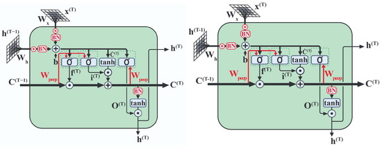
Figure 7.
ConvLSTM basic structure.
- = Input vector;
- = Memory from the previous block;
- = The output of the previous block;
- = Memory from the current block;
- = Output of current block;
- , , = Gates;
- = Sigmoid;
- = Weight;
- = Bias;Tanh = Hyperbolic tangent.
3. Simulation Designs
The parameters of the robot as well as its mass, center of floating, and moment of inertia can be found in the article [20]. The characteristics of the solver to carry out the simulations are shown in Table 3.
Table 3.
Solver characteristics.
To analyze the performance of the proposed predictor in terms of energy consumption, the RMS (Root Mean Square) value of the control coefficients used for the thrusters was calculated. These values were averaged to provide a representative measure of energy consumption. The equation to calculate RMS is
Simulation 1:
- ROV1 is the leader and ROV2 is the follower;
- The leader sensor has a 200 ms sampling period and there is no delay in data transmission between the leader and the follower;
- Helical trajectory;
- Leader–follower scheme;
- Various predictors are proposed: LS, MLP, LSTM, ConvLSTM, and Kalman predictor.
Simulation 2:
The simulations ran the following characteristics:
- ROV1 is the leader and ROV2 is the follower.
- The leader sensor has a sampling period of 200 ms and the transmission of information from the leader to the follower has a delay of 200 ms (to choose these values, we ran preliminary tests modifying the sampling time, the delay, and the currents; it was found that at 200 ms, they can be affected in different conditions and achieve the desired values);
- Helical trajectory;
- Leader–follower scheme;
- Various predictors are proposed: LS, MLP, LSTM, ConvLSTM, and Kalman predictor.
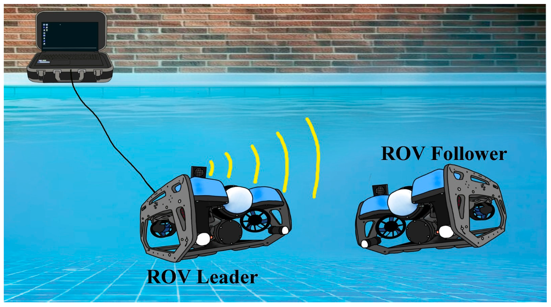
The objective of these simulations is to replicate communication using acoustic modems, with a latency and sensor sampling period of 200 ms, as illustrated in Figure 8. The simulations aim to accurately model the transmission and reception processes involved in acoustic modem communication, highlighting their performance under specified latency conditions and sensor data sampling intervals.

Figure 8.
Acoustic communication between leader and follower.
3.1. Ocean Currents
For the analysis of the system, marine currents are considered, which are described in detail in the work of Fossen [18]. It is assumed that these currents extend three-dimensionally and lack rotation, following the model proposed in said bibliographic reference.
where
The current velocity is identified as while the relative orientation of the currents is described by the angles of attack and slip angles . In the specific context, represents the current coming from the north, is that coming from the east, and is that arising from the depths, as illustrated in Figure 9.
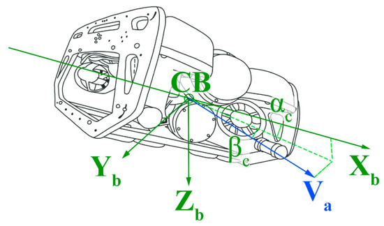
Figure 9.
Vector composition of marine currents.
To optimize the appreciation of the advantages between the different simulations, we suggest varying the current triangles and to capture changes more accurately in the marine environment and the adaptive capacity of the proposed predictors.
The values of ) and are established, with = 1.2. By substituting these values into Equations (39)–(41), they are presented as follows:
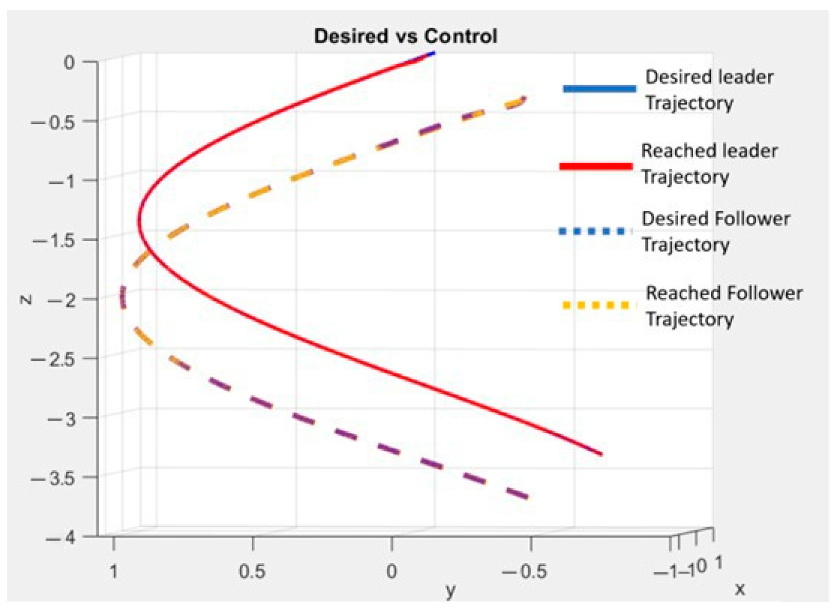
3.2. Trajectory
The planned path will take a spiral shape (Figure 10), as this involves changes in both positions and speeds along several axes, including forward motion, lateral displacement, ascent, and rotation. These positions, which must be controlled and monitored during movement, are defined by the coordinates w is constant and is the time of descent. Desired locations on the route will be identified as , while desired speeds will be represented as .
where are the desired position and is the desired angle.
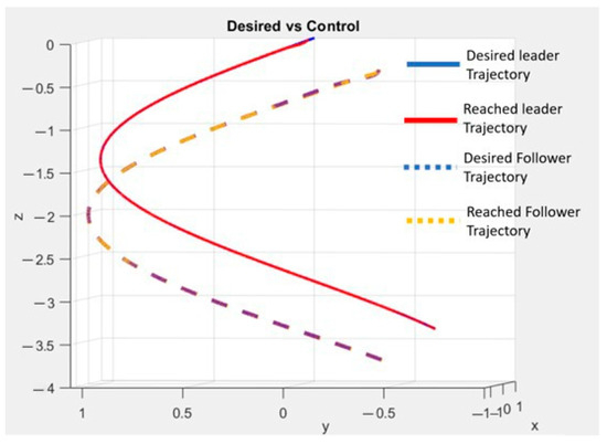
Figure 10.
Simulation trajectory.
Differentiating Equations (45)–(48) with respect to time gives
The values that were taken in the simulation are s y .
4. Simulation Results
4.1. Simulation 1
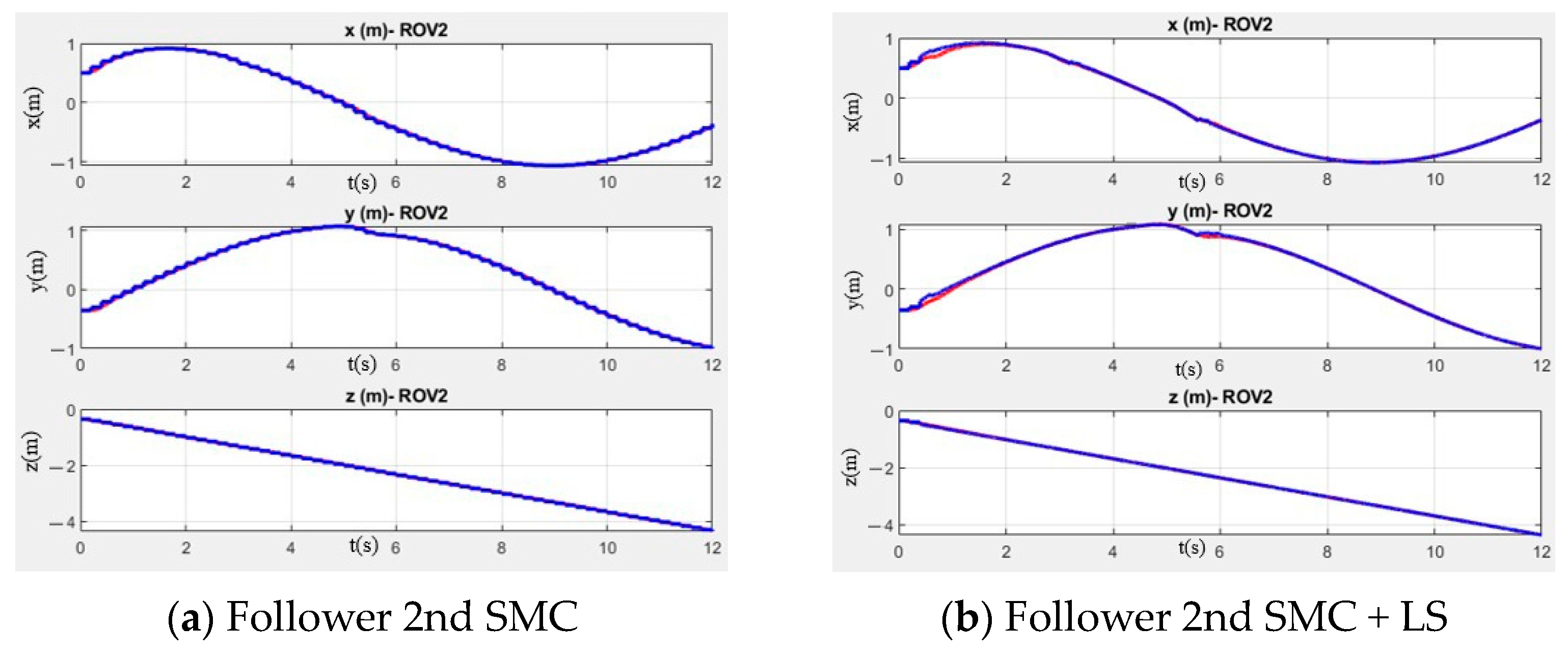
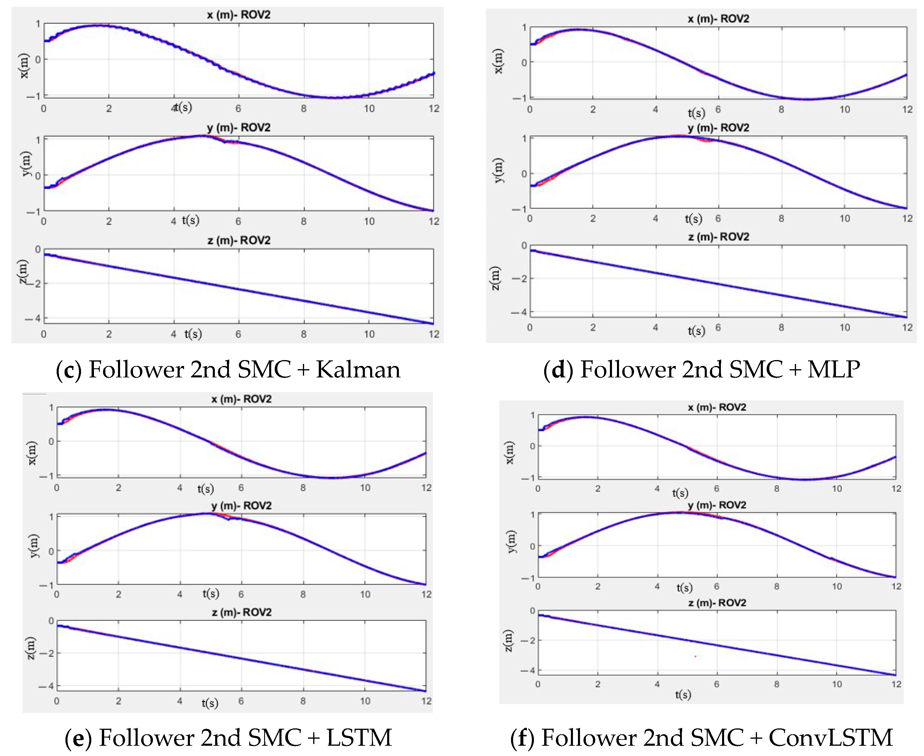
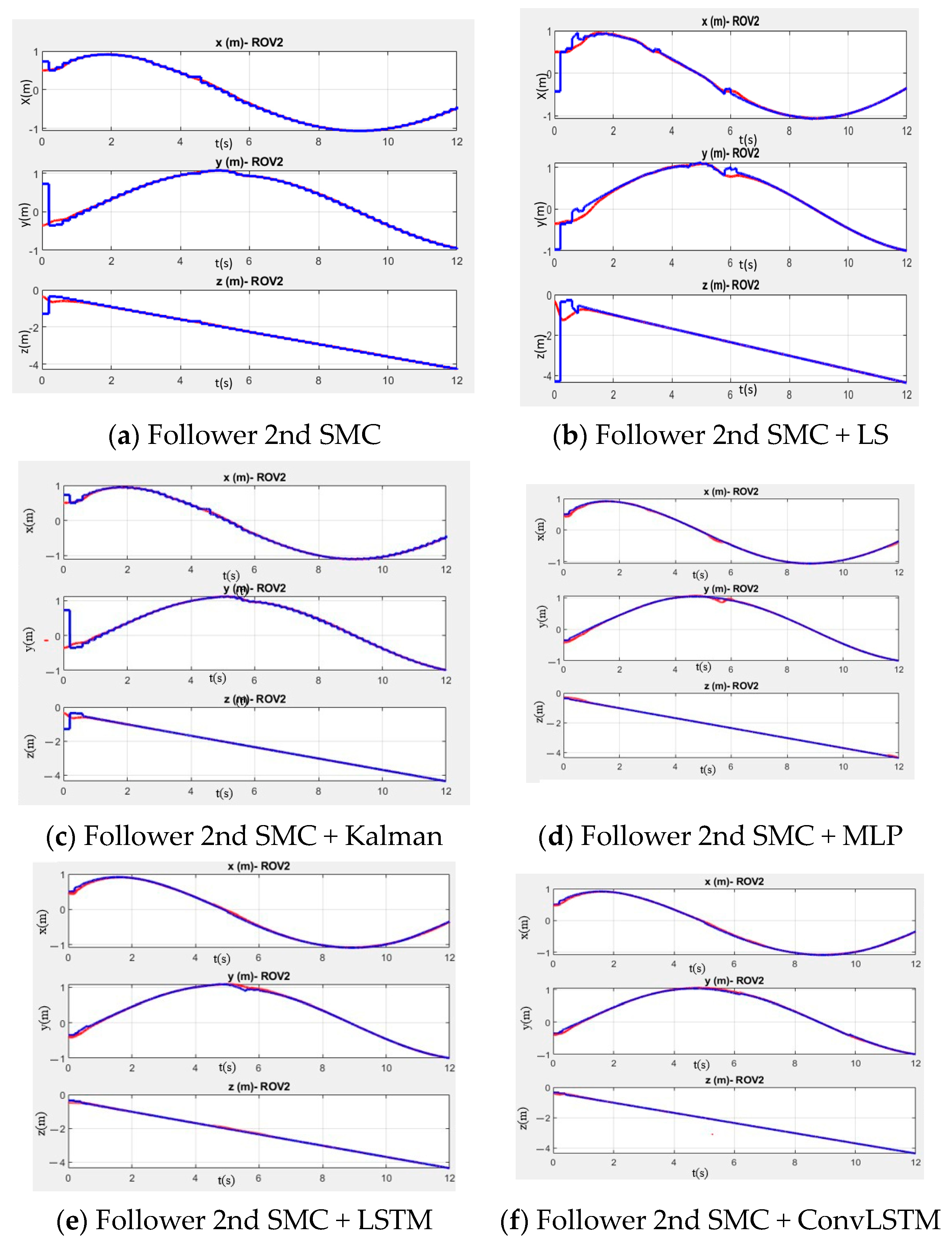
The blue lines represent the desired trajectories, while the red lines show the actual movement of the ROV follower. In the following simulations, only the results for ROV2, which is the follower robot, are presented. This is because ROV2 faces the biggest challenges in terms of communication, and this challenge is an area of opportunity.
Every 200 milliseconds (0.2 s), the ROV receives instantaneous information about its position. This means that the ROV is constantly adjusting its heading to try to follow the desired trajectory. However, due to this 200 ms update interval, the ROV may experience shattering when trying to reach its setpoint.
The influence of the variations on the results is made evident through graphical representations, which permit visualization of the oscillations generated due to the extensive sampling interval used. It is to be noted that both intelligent controllers and least squares methods demonstrate a considerable advantage in approximating the curves without saturating the motor outputs, as detailed in the analysis presented in Figure 11.
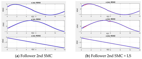
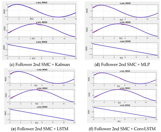
Figure 11.
Position simulation results of different predictors without ocean currents. The blue lines represent the desired trajectories, while the red lines show the actual movement.
In Figure 11, the desired trajectories are represented in blue, while the trajectories followed by the ROV are in red. Each position is indicated on the corresponding graphs. In Figure 12a, with a sampling period of 200 ms and without any predictor, a phenomenon known as shattering is observed, similar to that shown in Figure 12a. In Figure 12b–f, various predictors are implemented that help reduce noise and improve the approximation to the desired trajectories.
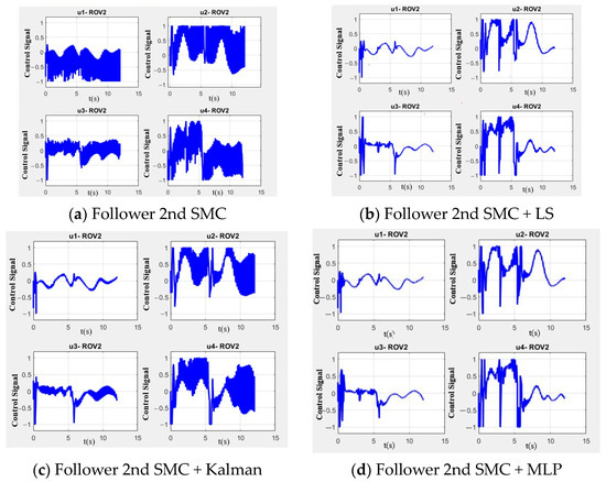
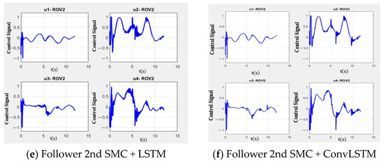
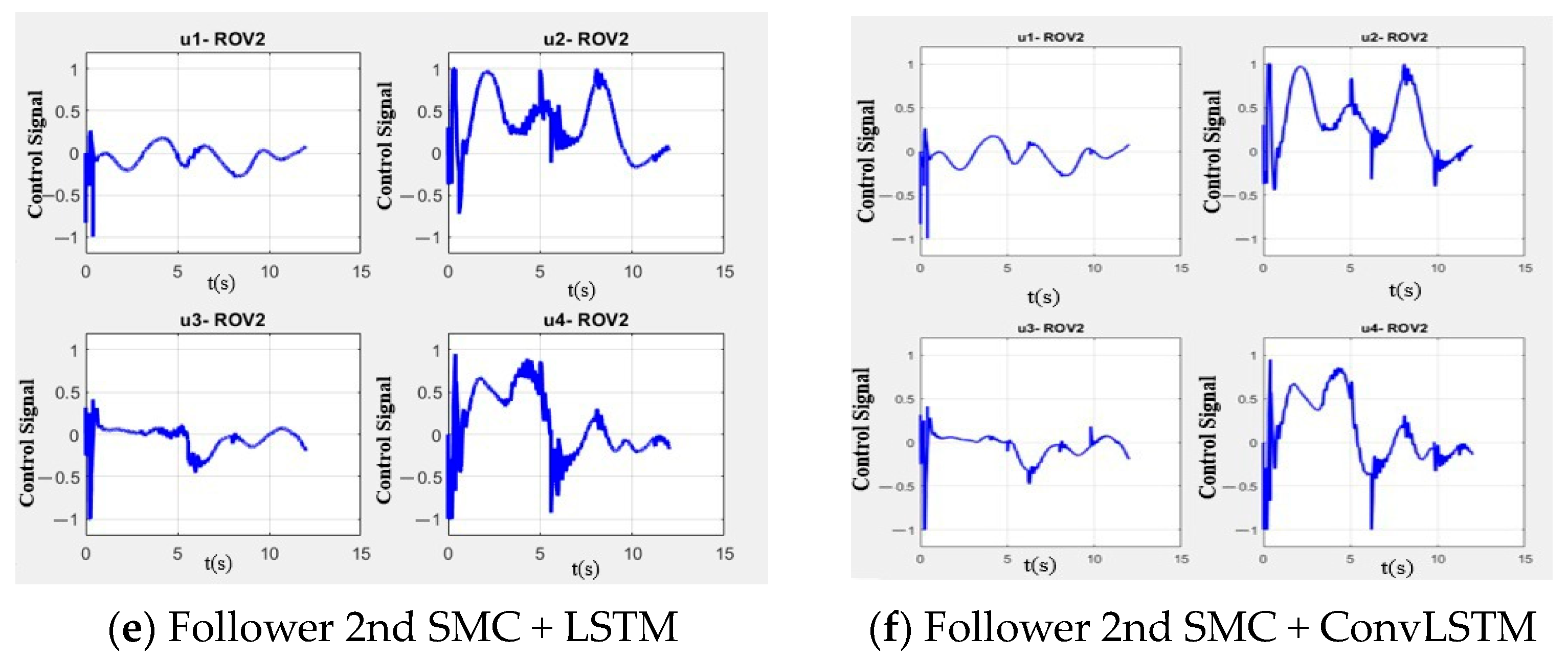
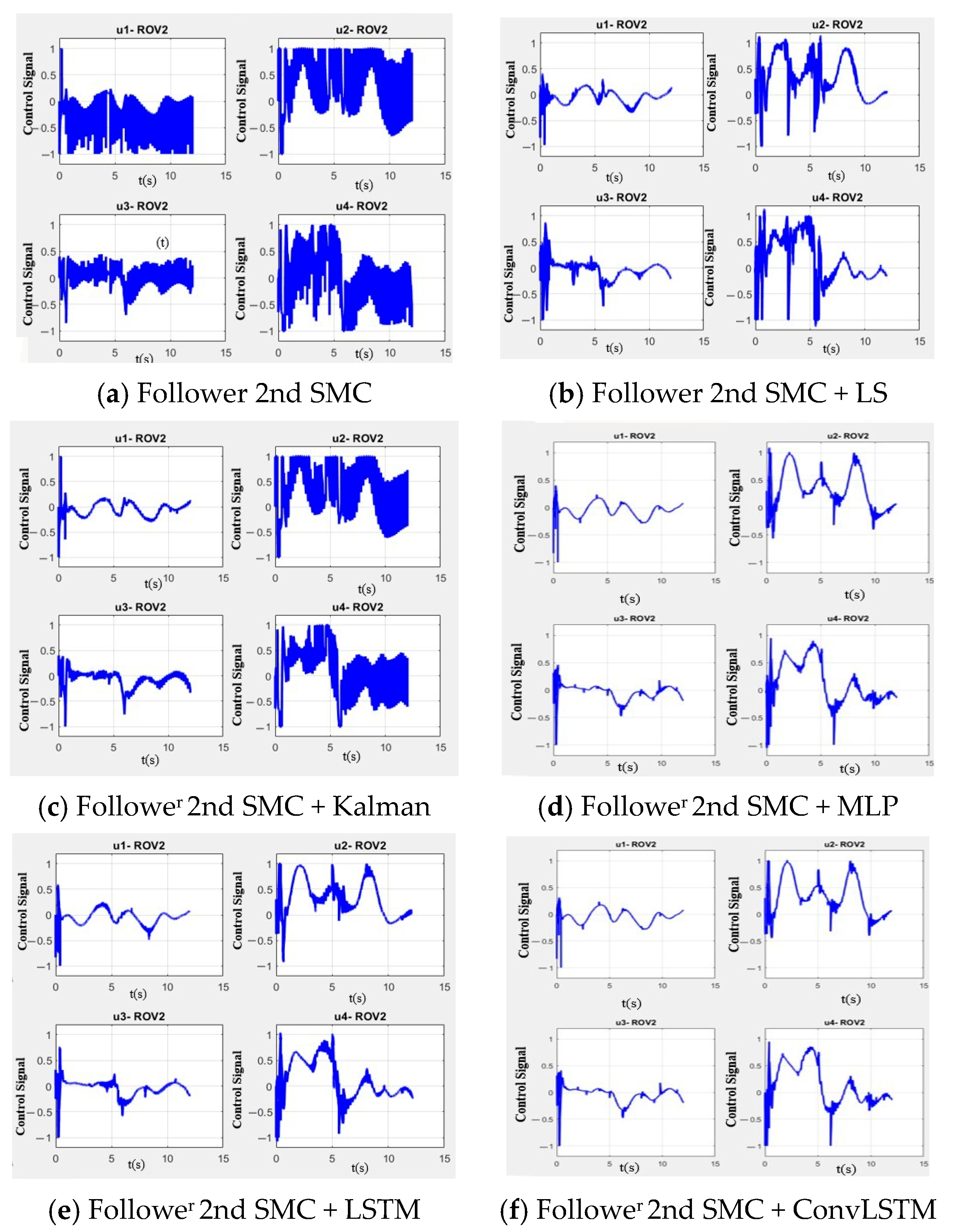
Figure 12.
Thruster simulation results of different predictors without ocean currents.
A significant aspect when considering these different predictors is the effect on the output signal, where the reduction in shattering results in a direct benefit to power consumption. As can be seen in Figure 12, output saturation and motor overload occur when no predictor is used, while in Figure 12b,c, an improvement is observed with the implementation of classic predictors. Modern predictors, as shown in Figure 12e,f, are better able to identify movement patterns, which significantly contributes to the reduction in chattering.
After completing the simulations, both the power consumption and the mean square error were calculated. In the first stage, the simulations were carried out excluding the influence of marine currents, as specified in the details of Table 2. Later, marine currents were incorporated into the simulations, and these data are reflected in Table 4.
Table 4.
Results without ocean currents.
The effects caused by the delay and the long sampling period result in oscillations and deviations from the desired value. Without the inclusion of predictors, these effects would be inevitable. However, by introducing predictors, significant improvements in the results are observed. Classic predictors show improvements, although not enough to completely avoid oscillations, while intelligent predictors achieve a more accurate prediction and avoid motor saturation more effectively (Table 4 and Table 5).
Table 5.
Results with ocean currents.
4.2. Simulation 2
The lines have the same representation as in the first simulation. In the second simulation, a communication delay is introduced. This causes the ROV to become static initially. To compensate for this delay, predictors are used to try to guess the ROV’s position. At first, due to the delay and lack of accurate data, the predictors may appear to start under different conditions. However, as more data are collected, the predictors adjust and improve their estimates of the ROV’s position.
The implementation of challenges such as sampling period and delay generates im-pulses that can affect the ability to reach the desired trajectory, as seen in Figure 13a and Figure 14a, where the motors can become saturated. An interesting finding is that by introducing time-varying changes in the direction and magnitude of the current, the classical predictors (Figure 14b,c) show more failures and a slight reduction in shattering in Figure 14b,c.
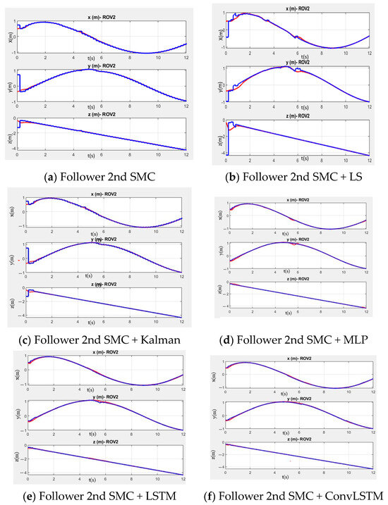
Figure 13.
Position simulation results of different predictors without changing ocean currents. The blue lines represent the desired trajectories, while the red lines show the actual movement.
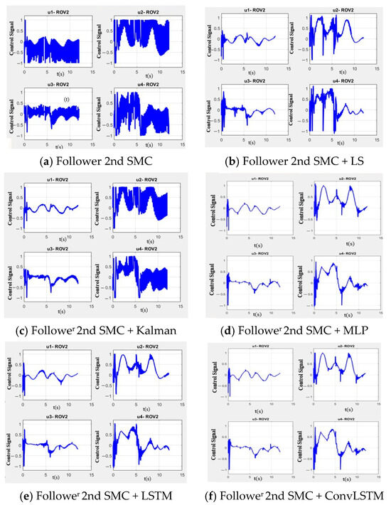
Figure 14.
Position simulation results of different predictors with changing ocean currents.
When predictors are implemented, a decrease in these effects is observed, although the improvements are not significant in Figure 14d,e. In contrast, ConvLSTM has the advantage of more easily detecting non-linear patterns in the system, resulting in a substantial reduction in shattering compared to other proposals.
In conclusion, the use of ConvLSTM stands out for its ability to effectively manage the challenges, notably improving the accuracy and stability of trajectory tracking in ad-verse environments.
In the next phase, simulations were performed without considering the influence of ocean currents, as shown in Table 6. Then, ocean currents were incorporated into the simulations, and the corresponding results are exhibited in Table 7, where the LSTM achieves better results.
Table 6.
Results without changing ocean currents and delay.
Table 7.
Results with changing ocean currents and delay.
5. Conclusions
In this work, simulations of a leader–follower scheme were performed, considering scenarios with inefficient communication, latency, and sampling periods of the sensors, as well as including changing ocean currents. To compensate for communication problems, a ConvLSTM network was implemented to perform trajectory tracking in a leader–follower scheme. A second-order sliding-mode control law was implemented on both robots to ensure convergence to the desired trajectories. Numerical simulations were implemented to evaluate the performance of the proposed ConvLSTM predictor, which has not been used for collaborative testing due to ineffective communication. The performance of the proposed network was compared with conventional and intelligent predictors. The predictors used for the comparison in this work are the Kalman filter, recursive least squares (LS), MLP, and LSTM. In the first simulations, having only a sampling period of 200 ms and the influence of currents, the data showed an improvement in trajectory tracking of 12.9% of the ConvLSTM network. In the second simulation, where the effect of communication latency is also considered, an improvement of 13.9% in trajectory tracking was obtained with the proposed network. Therefore, it presents a good capacity of the ConvLSTM network to significantly optimize performance and stability in collaborative operations between ROVs, especially in changing underwater environments. In addition, improved trajectory tracking reduces oscillations, which also reduces wear and damage to the motors.
In future research, new variables could be incorporated that could affect the communication between ROVs:
- These variables include environmental factors such as water pressure, temperature, and salinity or the consideration of information losses during transmission;
- The possibility of obstacles that could interfere with communication;
- Evaluating how increasing the number of ROVs could influence communication effectiveness;
- Exploring these additional variables could provide a more complete understanding of the challenges and potential solutions in underwater communication between ROVs.
Author Contributions
Conceptualization, J.G.-G., T.S.-J., L.G.G.-V. and A.G.-E.; methodology, L.G.G.-V. and T.S.-J.; investigation, M.E.P.-A.; software, J.G.-G. and M.E.P.-A.; writing—original draft preparation, M.E.P.-A.; visualization, M.E.P.-A.; writing—review and editing, L.G.G.-V., T.S.-J., A.G.-E., J.G.-G. and M.E.P.-A.; supervision, T.S.-J., J.G.-G., L.G.G.-V. and A.G.-E. All authors have read and agreed to the published version of the manuscript.
Funding
This research received no external funding.
Institutional Review Board Statement
Not applicable.
Informed Consent Statement
Not applicable.
Data Availability Statement
The data provided in this study are available upon request from the corresponding author.
Acknowledgments
The authors would like to acknowledge support from CONAHCYT for the MSc studies of the first author (scholarship number: 2201CA3003).
Conflicts of Interest
The authors declare no conflicts of interest.
References
- PI, R.; Cieślak, P.; Ridao, P.; Sanz, P. TWINBOT: Autonomous Underwater Cooperative Transportation. IEEE Access 2021, 9, 37668–37684. [Google Scholar] [CrossRef]
- Karras, G.; Kostas, K.; Kyriakopoulos, J. Towards Cooperation of Underwater Vehicles: A Leader-Follower Scheme Using Vision-based Implicit Communications. In Proceedings of the IEEE/RSJ International Conference on Intelligent Robots and Systems (IROS), Hamburg, Germany, 28 September–2 October 2015; pp. 1–6. [Google Scholar] [CrossRef]
- Simetti, E.; Casalino, G. Manipulation and Transportation with Cooperative Underwater Vehicle Manipulator Systems. IEEE J. Ocean. Eng. 2017, 42, 782–799. [Google Scholar] [CrossRef]
- Gao, Z.; Guo, G. Fixed-Time Leader-Follower Formation Control of Autonomous Underwater Vehicles with Event-Triggered Intermittent Communications. IEEE Access 2018, 6, 27902–27911. [Google Scholar] [CrossRef]
- Zhang, J.; Mou, J.; Chen, L.; Chen, P.; Li, M. Cooperative model predictive control for ship formation tracking with communication delays. Ocean. Eng. 2023, 291, 116272. [Google Scholar] [CrossRef]
- Huang, H.; Tang, J.; Zhang, B. Positioning Parameter Determination Based on Statistical Regression Applied to Autonomous Underwater Vehicle. Appl. Sci. 2021, 11, 7777. [Google Scholar] [CrossRef]
- Xu, J.; Qiao, L. Robust adaptive PID control of robot manipulator with bounded disturbances. Math. Probl. Eng. 2013, 2013, 535437. [Google Scholar] [CrossRef]
- Liu, M.; Tang, Q.; Li, Y.; Liu, C.; Yu, M. A Chattering-Suppression Sliding Mode Controller for an Underwater Manipulator Using Time Delay Estimation. J. Mar. Sci. Eng. 2023, 11, 1742. [Google Scholar] [CrossRef]
- Yu, Y.; Zhang, J.; Zhang, T. AUV Drift Track Prediction Method Based on a Modified Neural Network. Appl. Sci. 2022, 12, 12169. [Google Scholar] [CrossRef]
- Jin, X.; Yang, A.; Su, T.; Kong, J. GRU-Based Estimation Method Without the Prior Knowledge of the Noise. In Proceedings of the 11th International Conference on Modelling, Identification and Control (ICMIC2019), Harbin, China, 23–25 August 2019; pp. 927–935. [Google Scholar] [CrossRef]
- Hu, L.; Zhang, M.; Yuan, Z.-M.; Zheng, H.; Lv, W. Predictive Control of a Heaving Compensation System Based on Machine Learning Prediction Algorithm. J. Mar. Sci. Eng. 2023, 11, 821. [Google Scholar] [CrossRef]
- Sang-Kia, J.; Dea-Hyeong, J.; Ji-Youna, O.; Jung-Mina, S.; Hyeung-Sik, C. Disturbance learning controller design for unmanned surface vehicle using LSTM technique of recurrent neural network. J. Intell. Fuzzy Syst. 2021, 40, 8001–8011. [Google Scholar] [CrossRef]
- Wei, X.; Liu, Y.; Gao, S.; Wang, X.; Yue, H. An RNN-Based Delay-Guaranteed Monitoring Framework in Underwater Wireless Sensor Networks. IEEE Access 2019, 7, 25959–25971. [Google Scholar] [CrossRef]
- Gomez-Chavez, A.; Mueller, C.; Birk, A.; Babic, A.; Miskovic, N. Stereovision based diver pose estimation using LSTM recurrent neural networks for AUV navigation guidance. In Proceedings of the OCEANS 2017-Aberdeen, Aberdeen, UK, 19–22 June 2017; pp. 1–7. [Google Scholar] [CrossRef]
- Peng-Fei, L.; He, B.; Guo, J. Position Correction Model Based on Gated Hybrid RNN for AUV. IEEE Trans. Veh. Technol. 2021, 70, 5648–5657. [Google Scholar] [CrossRef]
- Liu, J.; Zhang, J.; Billah, M.M.; Zhang, T. ABiLSTM Based Prediction Model for AUV Trajectory. J. Mar. Sci. Eng. 2023, 11, 1295. [Google Scholar] [CrossRef]
- Wu, C.; Dai, Y.; Shan, L.; Zhu, Z. Date-Driven Tracking Control via Fuzzy-State Observer for AUV under Uncertain Disturbance and Time-Delay. J. Mar. Sci. Eng. 2023, 11, 207. [Google Scholar] [CrossRef]
- Fossen, T.I. Handbook of Marine Craft Hydrodynamics and Motion Control; John Wiley & Sons, Ltd.: Chichester, UK, 2011; ISBN 9781119994138. [Google Scholar]
- Rezaee, H.; Abdollahi, F. Synchronized Cross Coupled Sliding Mode Controllers for Cooperative UAVs with Communication Delays. In Proceedings of the 2012 IEEE 51st IEEE Conference on Decision and Control (CDC), Maui, HI, USA, 10–13 December 2012; pp. 1–6. [Google Scholar] [CrossRef]
- González-García, J.; Narcizo-Nuci, N.A.; García-Valdovinos, L.G.; Salgado-Jiménez, T.; Gómez-Espinosa, A.; Cuan-Urquizo, E.; Cabello, J.A.E. Model-Free High Order Sliding Mode Control with Finite-Time Tracking for Unmanned Underwater Vehicles. Appl. Sci. 2021, 11, 1836. [Google Scholar] [CrossRef]
- González-García, J.; Narcizo-Nuci, N.A.; Gómez-Espinosa, A.; García-Valdovinos, L.G.; Salgado-Jiménez, T. Finite-Time Controller for Coordinated Navigation of Unmanned Underwater Vehicles in a Collaborative Manipulation Task. Sensors 2023, 23, 239. [Google Scholar] [CrossRef] [PubMed]
- González-García, J.; Gómez-Espinosa, A.; García-Valdovinos, L.G.; Salgado-Jiménez, T.; Cuan-Urquizo, E.; Escobedo Cabello, J.A. Experimental Validation of a Model-Free High-Order Sliding Mode Controller with Finite-Time Convergence for Trajectory Tracking of Autonomous Underwater Vehicles. Sensors 2022, 22, 488. [Google Scholar] [CrossRef] [PubMed]
- Hansen, L.; Sargent, J. Recursive Models of Dynamic Linear Economies; Princeton University Press: Princeton, NJ, USA, 2005; ISBN 9780691042770. [Google Scholar]
- Grewal, M.; Andrews, A. Matlab-Kalman Filtering Theory and Practice Using MATLAB, 2nd ed.; Wiley: New York, NY, USA, 2001; ISBN 0-471-26638-8. [Google Scholar]
- Aggarwal, C. Neural Networks and Deep Learning: A Textbook; Springer: Berlin/Heidelberg, Germany, 2023; ISBN 978-3319944623. [Google Scholar]
- Chollet, F. Deep Learning with Python; Manning: Shelter Island, NY, USA, 2021; ISBN 978-1617294433. [Google Scholar]
- Hall, S.; Newman, S.; Loukaides, E.; Shokrani, A. ConvLSTM deep learning signal prediction for forecasting bending moment for tool condition monitoring. Procedia CIRP 2021, 107, 1071–1076. [Google Scholar] [CrossRef]


Disclaimer/Publisher’s Note: The statements, opinions and data contained in all publications are solely those of the individual author(s) and contributor(s) and not of MDPI and/or the editor(s). MDPI and/or the editor(s) disclaim responsibility for any injury to people or property resulting from any ideas, methods, instructions or products referred to in the content. |
© 2024 by the authors. Licensee MDPI, Basel, Switzerland. This article is an open access article distributed under the terms and conditions of the Creative Commons Attribution (CC BY) license (https://creativecommons.org/licenses/by/4.0/).