Abstract
Compared to traditional, static-based flywheel systems, vehicle-mounted magnetic suspension flywheels face more complex operating conditions, and existing control strategies usually regard disturbances in vehicles under different operating conditions to be the same problem. Therefore, it is necessary to determine the interference from complex operating conditions and reasonably distinguish among them under different operating conditions to provide flywheel systems with strong stability (the rotor offset was less than 0.025 mm). Thus, this paper proposes a high-stability control strategy for flywheels based on the classification of vehicle-driving conditions and designs its control strategy by taking the vehicle-mounted magnetic suspension flywheel with a virtual inertia spindle as an example. First, according to the different vehicle working conditions and the varying interference intensities affecting the flywheel system, the working mode is divided into four modes. Considering the obvious differences in each working mode, it is proposed to use BP neural network optimization based on the simulated annealing algorithm (SA-BPNN) to determine the flywheel’s working condition. A relatively simple neural network can improve the response speed of the whole system. It also has a good effect. Secondly, it is proposed to use deep learning models based on convolutional neural networks, long short-term memory networks and attention mechanisms (CNN+LSTM+ATTENTION) to train the corresponding control parameters under each working condition to judge and predict the control parameters under different working conditions. Three evaluation parameters are used to evaluate the training results, and all achieved good results. Finally, the classification of working conditions and performance tests are carried out. The experimental results show the effectiveness and superiority of the proposed control strategy.
1. Introduction
Flywheels, also known as flywheel energy storage systems, have the advantages of high energy storage conversion efficiencies, long lives, no pollution, and short charging times [1,2]. Flywheels are widely used in the shipping industry [3,4]. In the literature [5], a DC microgrid-system model for marine gas turbines was established, based on a 100 kW practical single-axis micro gas turbine engine. The model includes a micro gas turbine generator set, flywheel energy storage system (FESS), battery, propulsion load, and pulse load. References [6,7,8] describe the investigation and development of flywheel technology as energy storage systems for marine regional power systems. Reference [9], which focused on propeller rotations and waves, found that the high power and torque fluctuations in electric marine propulsion systems will affect the reliability of marine power networks and lead to wear and tear, and a new solution was proposed to solve load power fluctuations using a hybrid energy storage system (HESS) composed of a flywheel. Flywheels are also widely used in the automobile industry, having the dual functions of energy supply and braking energy recovery. Flywheels are mainly used in vehicles as auxiliary power supplies. When a vehicle accelerates, climbs, or requires instantaneous high-power output, the flywheel releases energy to power the vehicle and improve its performance. When the vehicle is in an emergency braking state, the energy utilization rate improves, and endurance increases. The adoption of flywheel technology can significantly improve the energy efficiency of electric vehicles [10,11,12].
The gyroscopic effect of a vehicle-mounted flywheel system is inevitable. Especially with the increase in the complexity of vehicle-driving conditions, the gyroscopic effect will become more pronounced, which makes flywheels prone to destabilization. Therefore, the requirements for a flywheel magnetic suspension system are very strict [13,14,15]. If the stability of the flywheel is not guaranteed under the continuous influence of the disturbance produced under complex vehicle-driving conditions, the unbalanced vibration of the flywheel itself will cause the generator to become eccentric over time, resulting in vibration, noise, and heating, which are also transmitted to the mechanical shell, resulting in the instability of the whole system [16,17,18,19].
At present, there are many studies on the use of control strategies to suppress flywheel vibration and realize the stable operation of a flywheel system. In Ref. [20], considering that the synchronous vibration and gyroscopic effect are two key factors affecting the overall stability of the flywheel in the full-speed region, a stability control method based on the golden frequency cross-sectional point is proposed to achieve such operation. In Ref. [21], which considered the influence of the real-time temperature on the speed of the flywheel, a multidimensional dynamic model involving temperature and speed variables, in addition to the traditional current and displacement, is proposed to realize the stable suspension of a flywheel system. In Ref. [22], which addressed the problems of inaccurate calculations of fringing flux and magnetic flux-leakage coefficient by existing modeling methods, a new modeling method based on the exact segmentation of the magnetic field was proposed, and the results of the performance comparison show that the control system based on the improved model had a stronger anti-disturbance characteristic than that based on a traditional model.
However, the above control strategies are based on a static model, without considering the influence of vehicle-driving conditions, and the disturbance caused by the vehicle itself is an essential link in the vehicle-mounted flywheel system, which cannot be ignored. Therefore, it is necessary to study high-stability control strategy of the flywheel under vehicle-driving conditions. In Ref. [23], a simplified test device for vehicle magnetic suspension flywheel system is proposed, which is designed to simulate vehicle-driving conditions through a series of sinusoidal and random vibration signals of different frequencies, and to study the dynamic response characteristics of flywheel under vehicle-driving conditions. In Ref. [24], through the analysis of the dynamic response of the flywheel in different forms of vehicle conditions, a dynamic correction model considering influence of vehicle-driving conditions is proposed, which has several sub models to cover as many driving conditions as possible. In Ref. [25], in order to solve the problem of the lack of detailed analysis of the characteristics of the same vehicle-driving condition in the existing studies, it is ignored that the stability of the flywheel system will change with the strength of the driving condition even under the influence of the same vehicle-driving condition. Therefore, a dual-mode coordinated control strategy according to favorable and poor vehicle-driving conditions is proposed.
At present, although there are many studies on the impacts of complex working conditions on vehicle-mounted flywheels, most are limited to certain road conditions [26]. In order to verify the stability of the established SMSFB support system, Ref. [27] analyzed the dynamic impacts of vehicle starting, acceleration, braking, deceleration, and uneven road surfaces on flywheels but without considering current road conditions. Various road parameters and current speeds have different levels of interference with flywheels. A complex, robust control method will lead to long response times by the flywheel control system, resulting in its failure to effectively control the flywheel in real time, resulting in an unstable working state of the flywheel over the long term, affecting its efficiency and life span. Therefore, a control strategy is urgently needed to solve this problem. The proportional–integral–differential (PID) controller, as a classic controller, has been widely used in flywheel systems [28]. It has a good control effect under simple working conditions, but in the face of complex working conditions, the PID control’s parameters must be adjusted in real time, resulting in a reduced control effect. A deep learning model is a kind of neural network model, which has strong complex function approximation and feature mining abilities. In order to solve the problems of the overdesign and insufficient precision of a CNN designed for attitude control system (ACS) fault diagnosis, the literature [29] proposes an improved particle swarm optimization (PSO) based on the new CNN architecture. For three-degrees-of-freedom, six-pole active magnetic bearings with strong coupling, nonlinearity, and unstable disturbance, an active disturbance rejection control strategy based on the BP neural network is proposed [30]. In order to ensure the frequency regulation of the power system and limit the energy level of the low-rated flywheel energy storage system (FESS), a nonlinear stepping neural adaptive predictive control system for a flywheel energy storage system based on a neural network is proposed for the frequency regulation of hybrid multizone power systems [31].
Therefore, in summary, most of the current research focuses on achieving the stable operation of flywheel rotor systems through innovative static modeling and suppression of synchronous vibration caused by gyroscopic effects. Although there have been studies on stability control strategies for flywheel systems under the influence of vehicle-operating conditions, the consideration of various driving conditions is not comprehensive enough. Most neural network control strategies for flywheels focus on improving energy utilization efficiency and frequency regulation of power systems, without considering stability control under the complex operating conditions faced by vehicle-mounted flywheels. Therefore, there is an urgent need for a control strategy that can comprehensively analyze the influences of complex operating conditions, scales of road conditions, and speeds on the stability of flywheels to ensure that whole flywheel system can operate stably under such conditions.
In this paper, a high-stability control strategy for vehicle-mounted flywheels based on SA-BPNN and CNN+LSTM+ATTENTION is proposed, and the control strategy is designed for a vehicle-mounted flywheel with a virtual inertial spindle. First, based on the flywheel prototype, the dynamics model of the flywheel is established using ADAMS/VIEW2020, and four typical complex vehicle-operating conditions (speed bumps, turns, ramps, and sudden pedestrians) are simulated in ADAMS/CAR2020 to analyze the operating characteristics of the flywheel under various vehicle-operating conditions. The working condition interference data are input into the SA-BPNN to conduct working mode training, which is used to determine the current working mode of the flywheel. Then, according to the disturbance in the summarized flywheel under different vehicle-driving conditions, by introducing the corresponding vehicle-driving condition factors, the working conditions data are input into the LSTM+ATTENTION for training, and the control parameters of the response are trained according to the different working conditions. Finally, condition classification and performance tests are carried out to verify the superiority of the proposed control strategy.
2. Classification of Vehicle-Driving Conditions
2.1. Significance of Classification of Vehicle-Driving Conditions
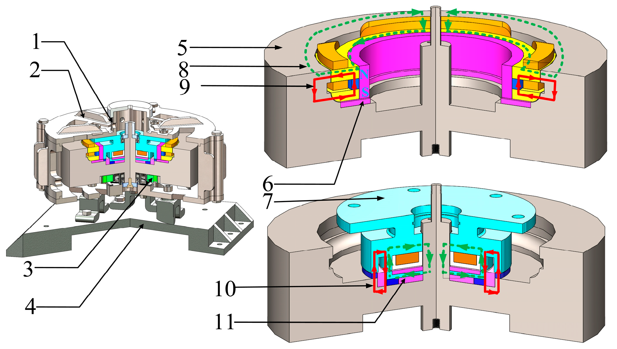
The overall structure and magnetic circuit of the vehicle-mounted flywheel system based on a virtual inertial spindle are shown in Figure 1. See Reference [18] for details of the structure and magnetic circuit.
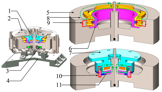
Figure 1.
Overall structure and magnetic circuits of the vehicle-mounted flywheel: (1) sensor mounting hole; (2) housing; (3) motor; (4) foundation; (5) flywheel; (6) radial magnetic bearing; (7) axial magnetic bearing; (8) radial control flux; (9) radial biased flux; (10) axial biased flux; (11) axial control flux.
Research on traditional stability control strategies for flywheel systems mainly focus on stability analyses and controller designs for single-system flywheel models. However, in the actual operation of a flywheel system, the interference from various vehicle-driving conditions and the process of switching the flywheel’s operating mode often cause the system to jump from its original operating point to a new operating point. Moreover, the transient error at the jump time is often large, and the convergence speed of the identification algorithm is reduced. Therefore, it is difficult to use a single, linear, and time-invariant controller and meet the requirements of high-precision control and system stability. Therefore, it is better to classify and model the system based on the influence of different vehicle-driving conditions on the original model (static model); that is, the adoption of a multimodel adaptive control method can allow the flywheel system to cope efficiently with external disturbances, such as changes and switches in vehicle-driving conditions, and achieve high stability control of the flywheel.
2.2. Rough Classification of Vehicle-Driving Conditions
First, the original model, which is the basis of the condition classification and does not consider the vehicle condition, is shown below:
where the flywheel is assumed to be offset in both the radial and axial directions, with offsets x0, y0, and z0, respectively, in the positive directions of the x-axis, y-axis, and z-axis of the reference coordinate system; kx and ky are the radial statics-displacement stiffnesses; kix and kiy are the radial statics–current stiffness; kz and kiz are the axial statics–displacement stiffness and axial force–current stiffness, respectively; x0, y0, and z0 are the radial and axial offset values of the flywheel measured by the position sensor in the basic static state, respectively; ix0, iy0, and iz0 are the radial and axial control currents at static states, respectively; µ0 is the permeability of the vacuum; N1 and N2 are the effective turns of the radial equivalent three-phase coil and the effective turns of the axial coil, respectively; Fm1, Fm2, and Fm3 are the magnetic potentials generated by radial permanent magnets, outer-ring axial permanent magnets, and inner-ring axial permanent magnets, respectively; Sr, Sr2, Sa1, and Sa2 are radial upper-stator polar segment, radial lower-stator polar segment, axial stator transverse segment, and axial stator inner segment, respectively; and δr, δa1, and δa2 are the radial, axial, and axial uniform air gap lengths of the flywheel without eccentricity respectively.
Second, based on the basic static model, the characteristics of the model according to the various vehicle-driving conditions need to be further analyzed in order to better implement the multimodel adaptive control strategy.
When the flywheel is disturbed by the vehicle’s own driving conditions, it will deviate from the center. According to the disturbance from external vehicle-driving conditions, the eccentric phenomenon can show different characteristics through a displacement deviation of three degrees of freedom. Therefore, according to a dynamic simulation, analyzing the displacement deviation by three degrees of freedom under various vehicle-driving conditions is helpful for distinguishing a vehicle’s movement conditions.
Based on the above static model, as shown in (1), a comprehensive dynamics analysis was carried out and a dynamic model that considers the influence of vehicle conditions is supplemented and amended. When the vehicle runs under different vehicle-driving conditions, the flywheel will deviate in the radial and axial directions due to the external disturbance. This is called the base offset. At this point, the coil will generate an additional current by controlling the movement of the system through the magnetic bearing. This is the compensating current. The radial and axial suspension forces are changed to balance the effect of the base offset. The base offset and compensation can be expressed as follows:
where Δxf, Δyf, and Δzf are the base offsets; Δifx, Δify, and Δifz are the radial and axial compensation currents, respectively; kf1 and kf2 are the radial and axial basic weight factors, respectively, and their values depend on different basic motion modes; t is the basic running time; ξ is the median of the integral; af(t) is the basic acceleration equation; ix0, iy0, and iz0 are the static radial and axial currents; ix, iy, and iz are the radial and axial currents after deviation; ux0, uy0, and uz0 are the static radial and axial voltages; ux, uy, and uz are the radial and axial voltages after deviation; and Rc1 and Rc2 are the resistances of the radial and axial coils.
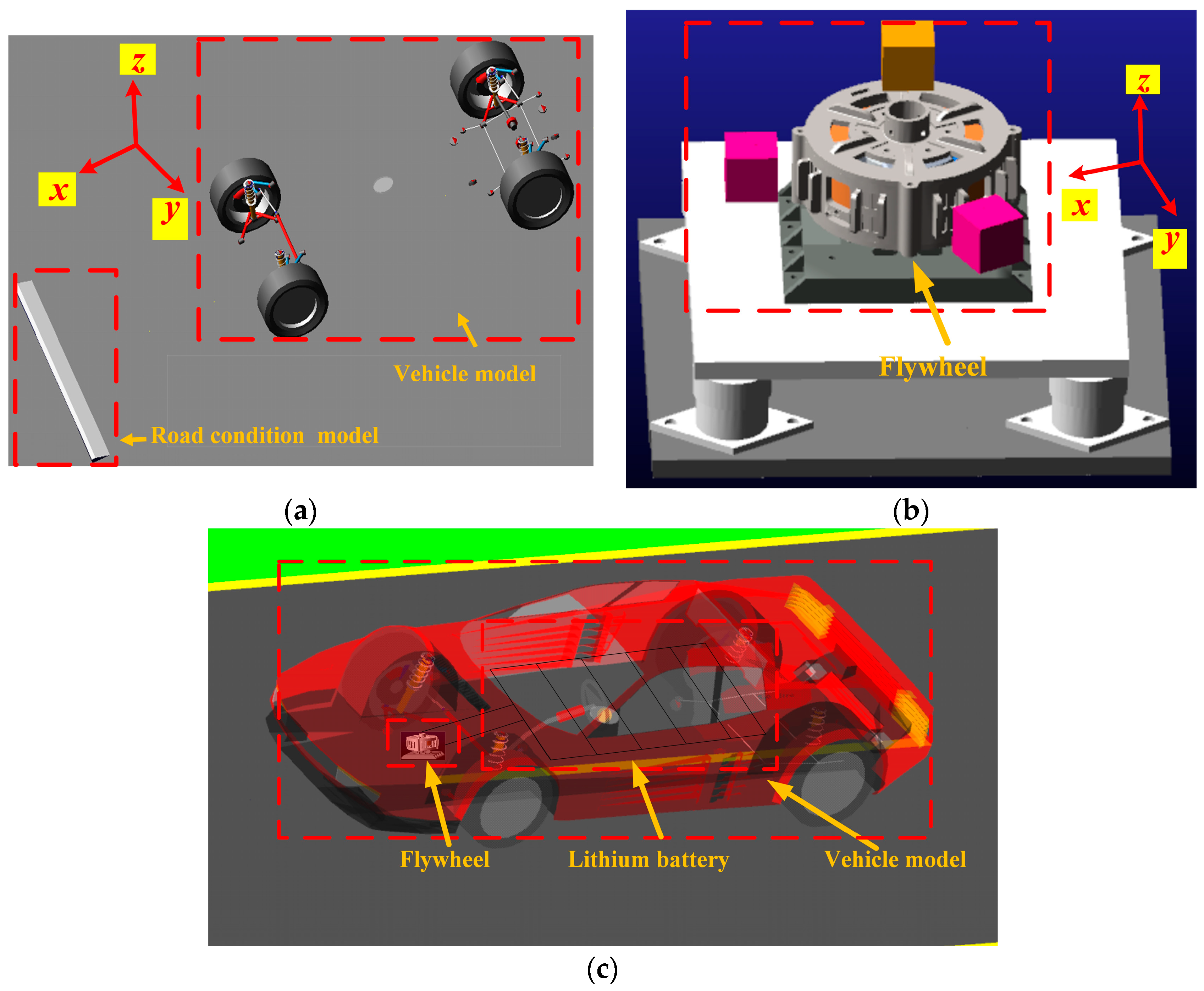
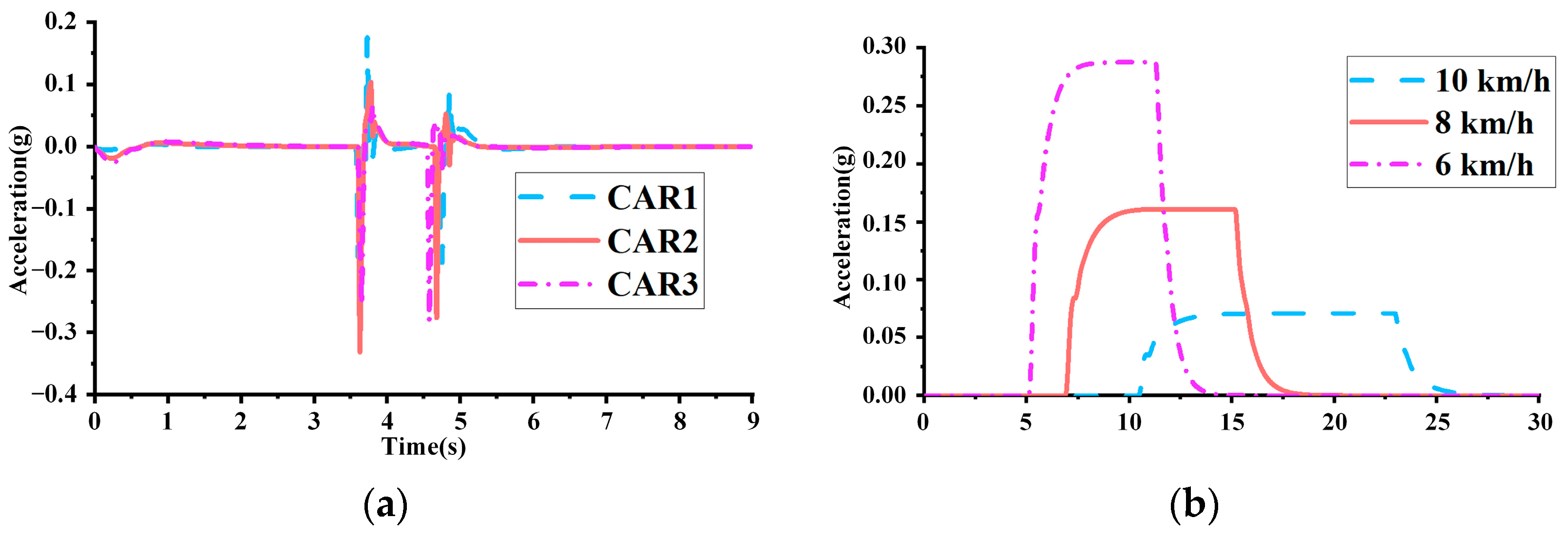
Then, based on the dynamics model of (1) and (2), ADAMS/CAR2020 is used to establish a working condition model, the acceleration under the current complex working condition is imported into the ADAMS/VIEW2020 flywheel model, and the flywheel deflection characteristics under complex working conditions are analyzed in ADAMS/VIEW2020 software, and the forward direction of the vehicle is simulated as x. Align with the x-axis of the flywheel, as shown in Figure 2. Four common complex operating condition models are built in ADAMS/CAR2020, which are driving over a speed bump; turning; driving uphill; and sudden pedestrian encounters (sudden braking). In these four models, the vehicle mass, size, spring, suspension stiffness, and road condition parameters in ADAMS/CAR2020 are analyzed in detail. Figure 3 shows the lateral acceleration curves of vehicles with different parameters crossing 4 cm deceleration belts at 10 km/h and the lateral acceleration curves with a turning radius of 10 m at different speeds.

Figure 2.
Vehicle-driving conditions in the simulation: (a) vehicle model and road condition model; (b) flywheel; (c) flywheel, lithium battery, and vehicle model.
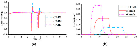
Figure 3.
Dynamic characteristic curves of a flywheel rotor under different working conditions: (a) speed bump; (b) turning.
3. High-Stability Control Strategy for Flywheels Based on Classification of Vehicle-Driving Conditions
According to the simulation’s results in Figure 3, it can be seen that the vehicle-mounted flywheel was subject to interference from different factors during actual operation, and different interference factors will cause interference of different sizes and directions. Therefore, in order to further improve the accuracy in determining the operating conditions of a flywheel, different factors under various working conditions are simulated, and the acceleration in each direction is recorded. A simulated annealing BP neural network was used for training on both the training set and test set, and the working mode of the flywheel was determined according to the acceleration data in each direction. Among them, the speed bump road condition is set as working mode I, the turning road condition is set as working mode II, the ramp road condition is set as working mode III, and traffic interference is set as working mode IV.
The BP neural network model has a strong nonlinear fitting ability, but the BP neural network may have local minimum, which will greatly affect the accuracy of the model’s predictions. The simulated annealing algorithm can jump out of the local optimal and find the global optimal solution. Therefore, this paper introduces a simulated annealing algorithm to determine the parameters of the BP neural network, optimize the BP neural network, and build a simulated annealing optimized BP neural network model.
The simulated annealing algorithm consists of the following two parts: Metropolis algorithm and annealing process. These two parts correspond to the inner cycle and the outer cycle. The Metropolis criterion accepts deteriorating solutions with a certain probability, which causes the algorithm to jump out of the locally optimal trap.
Assuming that the previous state is x(n), the state of the system changes to x(n+1) according to a certain index (gradient descent and energy in Section 1), and correspondingly, the energy of the system changes from E(n) to E(n+1), the acceptance probability P of the system changing from x(n) to x(n+1) is defined as follows:
The specific process is as follows:
- (1)
- Divide the sampled data on the control parameters under each working condition, as follows, divide the sample data into training sample data and test sample number
- (2)
- Normalize the sample data.
- (3)
- Select the parameters for the BP neural network; that is, determine the network parameters and activation functions of the neural network. Initialize the weights and thresholds of the BP neural network.
- (4)
- Calculate the error, that is, calculate the mean squared error between the actual output and the expected output of the network.
- (5)
- Initialize the parameter of the simulated annealing algorithm; that is, maximum temperature, T0; minimum temperature, Tmin; annealing rate | and step size factor.
- (6)
- Call the simulated annealing algorithm to correct the weights and thresholds of the BP neural network, as follows:
- (7)
- Re-calculate the error, that is, calculate the mean squared error between the actual output and the expected output of the network.
- (8)
- Determine whether the increment is less than 0. If it is less than 0, accept the new solution; otherwise, determine exp(−△MSE/T)>rand ? If it is true, accept the new solution; if it is not true, judge whether the number of iterations has been reached; if it is not reached, return to step (6); if it is reached, judge the condition.
- (9)
- Determine whether the termination condition is met; if it is met, proceed to step (10); and if it is not met, call the temperature to step (6).
- (10)
- Input the test sample data and obtain the prediction result on the trained neural network.
The parameters of the simulated annealing algorithm are shown in Table 1.

Table 1.
Simulated annealing algorithm’s parameters.
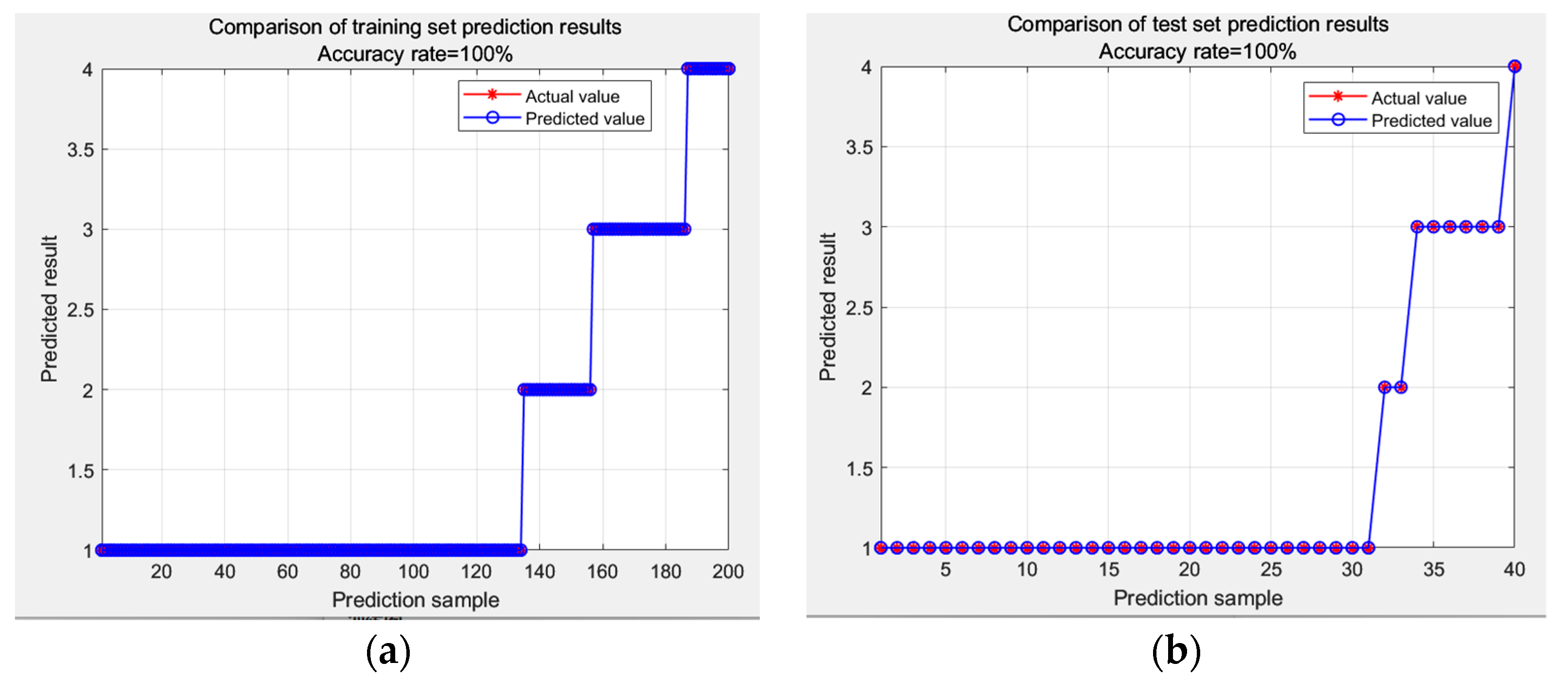
As shown in Figure 4, it can be seen that the simulated annealing BP neural network could determine the operating mode of the flywheel well (accuracy rate = 100%), and the relatively simple neural network can determine the operating mode of the flywheel, which greatly reduces the complexity of the whole system and speeds up its response speed.
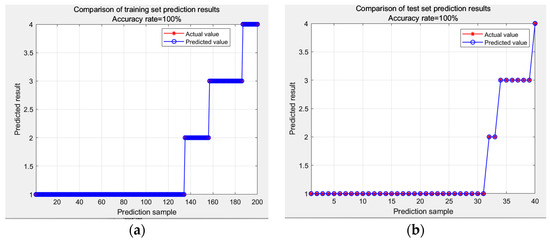
Figure 4.
Simulated annealing BP neural network training set prediction results and test set training results: (a) comparison of training set prediction results; (b) comparison of test set prediction results.
3.1. High-Stability Control Strategy for a Flywheel
According to the classification of the vehicle-driving conditions analyzed above, the characteristics of each degree of freedom under different operating conditions can be obtained. Displacement deviation values caused by disturbances under different working conditions can differ by ten times. Therefore, it is difficult to use controllers with the same parameters to meet the control requirements under complex working conditions. To ensure stable control under different vehicle-driving conditions, it is necessary to have a controller with the most suitable control parameters under each classification. Therefore, a high-stability control strategy based on the classification of vehicle-driving conditions is proposed.
- (1)
- CNN
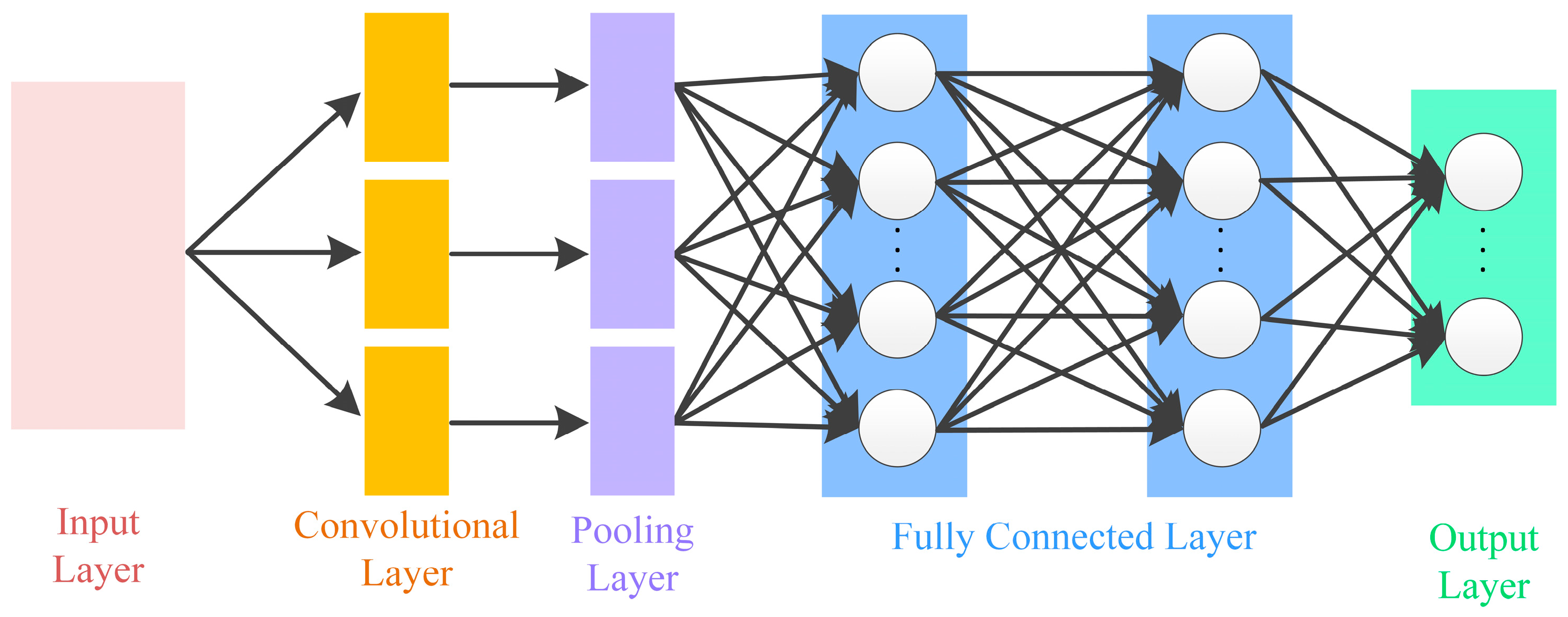
A CNN is a deep feedforward neural network. The core structure of a CNN is shown in Figure 5. Using a convolution kernel to carry out the convolution operation, the data are mapped nonlinearly through the excitation layer. The data are then obtained through the pooling layer, and the resulting feed goes into the fully connected layer. Finally, the loss function is calculated to update the network parameters. In particular, the convolutional layer of the CNN is the key to extracting features, and it consists of multiple learnable filters.

Figure 5.
CNN structural diagram.
In terms of extracting the spatial attributes of the input data, the convolutional layer performs discrete convolution operations on the data. The pooling layer takes the maximum or average value of the convolution results, thereby reducing the spatial dimensions of the data volume. Thus, the key information is extracted and irrelevant information eliminated.
- (2)
- LSTM
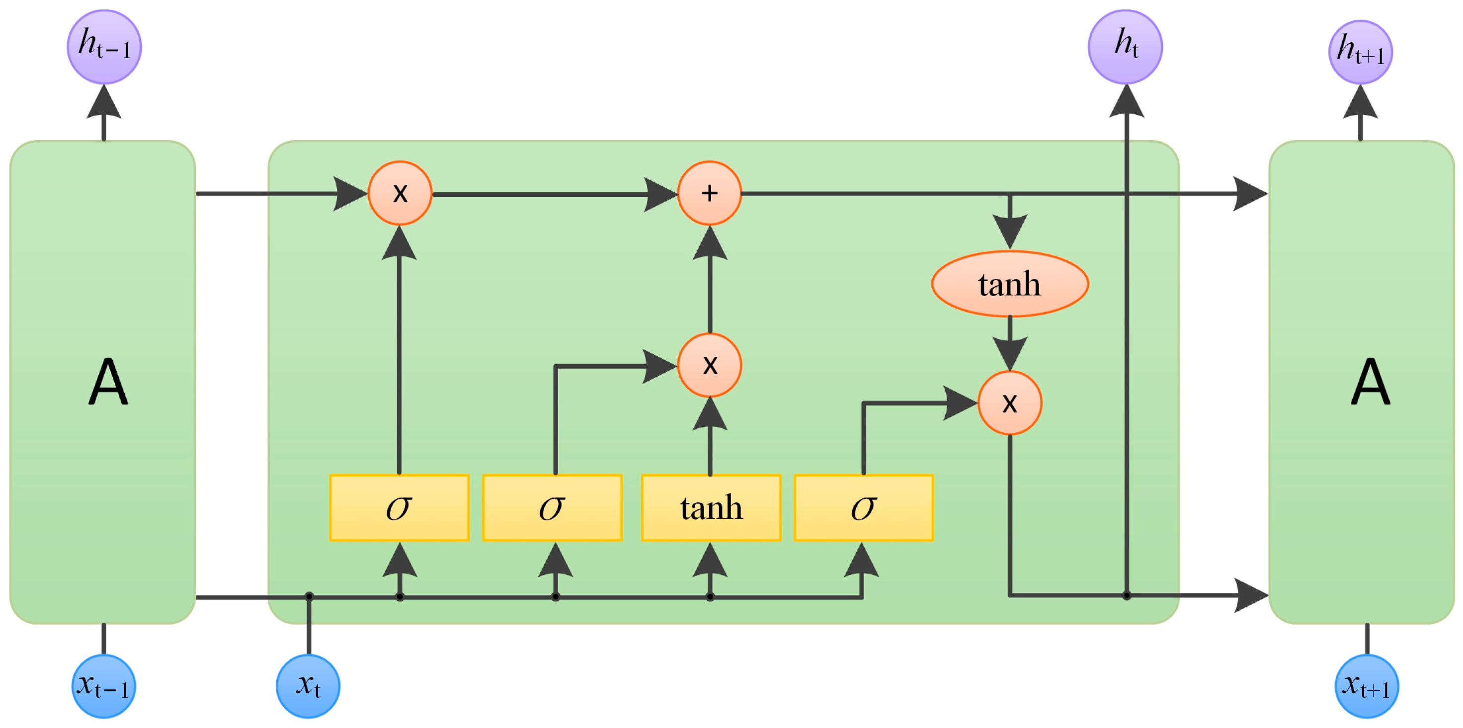
LSTM is a special type of recurrent neural network (RNN) that is mainly used to process sequential data, such as time series data and natural language processing tasks. It can effectively solve the problems of gradient disappearance and gradient explosion faced by traditional RNNs when processing long sequence data to better capture long-term dependency. It consists of a series of memory units. Each memory unit contains the following three main gating structures: input gate, it; forget gate, ft; and output gate, ot.
where Wi, bi, Wf, bf, Wo, and bo are the weight matrix and bias vector parameters to be trained; is the new candidate value vector; and Ct is the current cell state. In addition, σ means that the sigmoid function is as follows:
The performance of the LSTM model is measured by the mean error (MAE) and mean squared error (MSE), and the decisive coefficient (R2) is added for measurement, as described in Equations (12)–(14); n represents the number of sample points in the test set; m represents the number of sample points in the training set; is the basic truth value; is the predicted value by the machine learning model; and is the average of the values predicted by its learning model. These metrics provide a quantifiable way to assess the accuracy of the model’s predictions.
The interference with the flywheel in this study is characterized by a time series, in which the observed results are used to predict the rotor offset of the flywheel under certain conditions in the future, and the performance of the model is evaluated by the indexes of MSE, MAE, and R2. The effectiveness of the CNN+LSTM+ATTENTION model and its potential for use in flywheel control applications can be evaluated. The specific structure is shown in Figure 6.
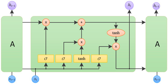
Figure 6.
LSTM structural diagram. Where A represents the LSTM model, + represents addition, and x represents multiplication, t − 1 is the last time, t + 1 represents the next moment.
The interference with the flywheel in this study is characterized by a time series, in which the observed results are used to predict the rotor offset of the flywheel under certain conditions in the future. The performance of the model is evaluated by the indexes MSE, MAE, and R2. The effectiveness of the CNN+LSTM+ATTENTION model and its potential for use in flywheel control applications can be evaluated.
- (3)
- Attention Mechanism
The main goal of the attention mechanism is to simulate the way humans allocate attention during information processing. The key is to make the model focus on valuable information and filter out irrelevant information so that key features can be extracted from a large amount of information. The attention mechanism uses a probability allocation method, which can replace the method of assigning probabilities to randomly assigned initial weights.
Given k eigenvectors hi (i = 1, 2,…, k), the model can use hi to determine the environment vector ci. The equation for ci is as follows:
where ai is the attention weight, represented by the softmax function, and hi represents the output of each hidden layer.
ai = softmax(Si)
- (4)
- SA-BPNN combined with CNN+LSTM+ATTENTION
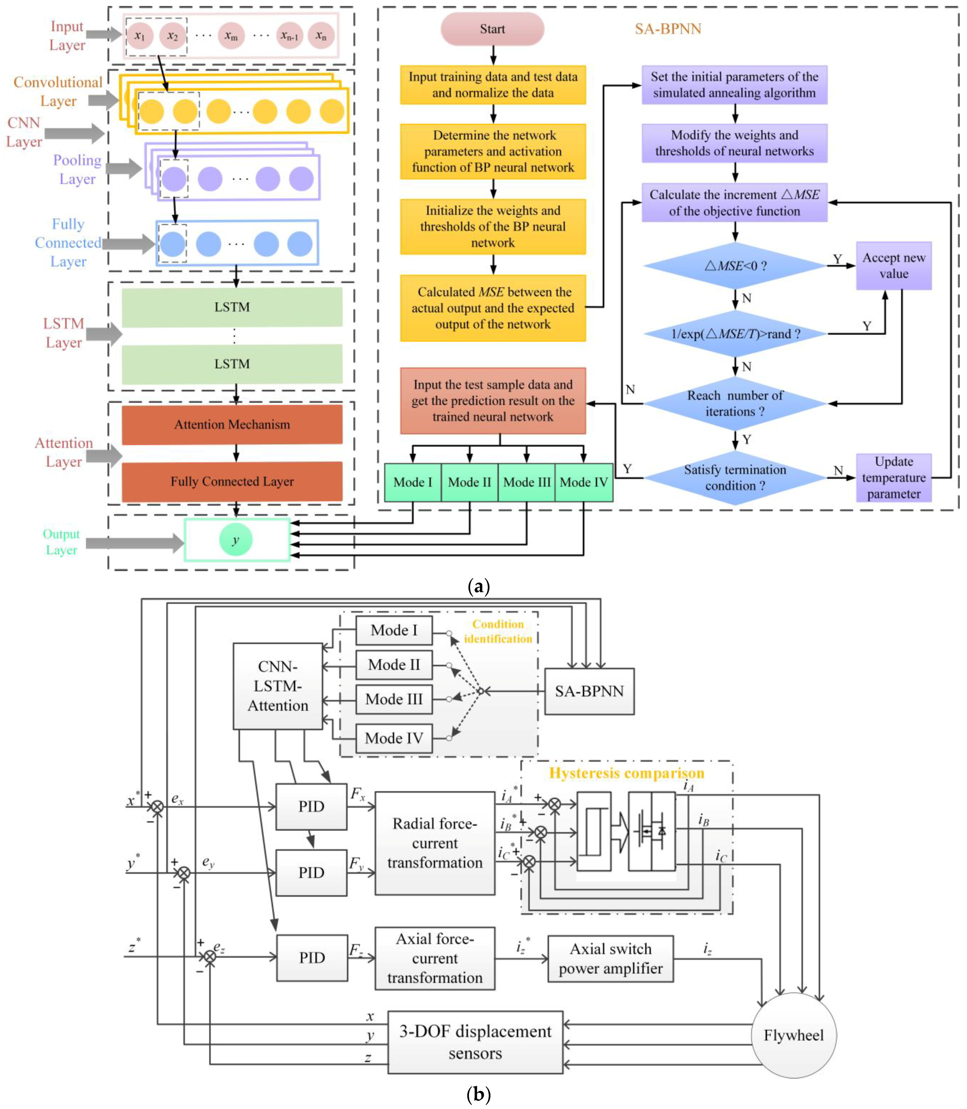
The CNN+LSTM+ATTENTION is divided into five layers. The first layer is the input layer, and the second layer is the CNN layer, which extracts the spatial relationships among different feature values in the data and making up for the determinations of the LSTM. The third layer is the LSTM layer, which has the memory function. The fourth layer is the attention layer, which can improve the roles of important time steps in the LSTM, thus improving the accuracy of the model’s predictions. The fifth layer is the output layer.
Together with the above SA-BPNN working pattern recognition and basic flywheel control system, a high-precision control strategy is formed. The specific structure is shown in Figure 7.

Figure 7.
High-precision control strategy: (a) flowchart of the SA-BPNN combined with CNN+LSTM+ATTENTION; (b) control diagram. Where x*, y*, z* represents the displacement signal in radial x, radial y, and axial z signal, iA*, iB*, iC* indicates three-phase circuit by radial force-current transformation, iz* indicates axial circuit by axial force-current transformation, + means addition, − means subtraction, ⊗ means comparison point, dashed lines indicates that the modules in the dashed line form a module.
It is worth noting that the two deep learning models are superimposed, and the following problems arise:
- Increased complexity of the model: If two models with different architectures are directly combined, the complexity of the overall model will greatly increase. This means that more computing resources and time are needed to train and optimize the model, and the requirements of the hardware equipment will become higher.
- Increased difficulty in parameter adjustment: There are more parameters that need to be adjusted, such as the initial temperature, attenuation coefficient, and other parameters in the SA-BPNN; the convolution kernel size in the CNN+LSTM+ATTENTION; the number of LSTM units; and the weight of the attention mechanism. Finding an optimal set of parameters becomes more difficult.
- It is difficult to determine how to effectively integrate the SA-BPNN with the CNN+LSTM+ATTENTION. Different fusion methods can have a big impact on the performance of the model. For example, whether to integrate at the feature level or at the decision level needs to be decided according to the requirements and data related to specific target tasks.
- Increased training data requirements: Complex combinatorial models often require large amounts of data for effective training. If the flywheel condition data are insufficient, it may result in overfitting, or the model cannot adequately learn effective feature representations.
- Increased risk of overfitting: Complex models are more prone to overfitting. Although the risk of overfitting can be alleviated by regularization, in practical applications, it is also necessary to ensure that the model has good fitting ability with different flywheels.
In view of the above difficulties, we implemented the following solutions:
- In view of the problem of the increasing complexity of the model, we innovatively divide the flywheel control system into two modules; one is the condition determination module, and the other is the control parameter adjustment module. Because of the complexity of the data processing required by the two modules, the SA-BPNN is used as the condition determination module. Using the CNN+LSTM+ATTENTION as the control parameter adjustment module, the two modules can be trained separately in their own modules, which greatly reduces the complexity of the model.
- In view of the increasing difficulty in parameter adjustments, the model corresponding to the work judgment module and the control parameter adjustment module is trained extensively, and the key parameters in each model are adjusted according to the training results until the results meet the performance requirements.
- In view of the problem of how to effectively integrate the two models, we innovatively applied the two models to the two modules of the flywheel system and fused the output layer of the two models to determine the operating mode of the current flywheel and the control parameters corresponding to the current mode to ensure its stability. In the face of flywheels with different rotation masses, materials, shapes, and motors, just changing the parameters of the data set required for training can make accurate working condition judgment and stability control.
- In order to increase the required training data and increase the risk of overfitting, we built various complex conditions in ADAMS/CAR2020 according to the complex conditions to be analyzed, and took into account the different interference intensities from various road conditions and speeds on the flywheel under complex conditions. In the same complex working condition, different road condition specifications and speeds are set, and the co-simulation with ADAMS/VIEW2020 is carried out to obtain the interference caused by the flywheel, which is used as the data set for the working condition judgment. In addition, radial and axial PID control parameters of the flywheel under different working conditions are obtained according to the interference size, which are used as the data set for the control parameter adjustment module. Not only can the model learn more essential features and laws in the data to handle complex conditions in real life, but it also solves the problem of having insufficient data to meet the requirements of the model and overfitting.
After solving the above problems, the four working modes are analyzed in detail.
3.2. Mode I (Speed Bump Condition)
Set the spring mass, damping ratio, and suspension stiffness of the common models in ADAMS/CAR2020; the specific parameters are shown in Table 2:
Table 2.
Vehicle structure parameters.
Set the speed bump in ADAMS/CAR2020; the speed bump parameters are shown in Table 3:
Table 3.
Speed bump parameters.
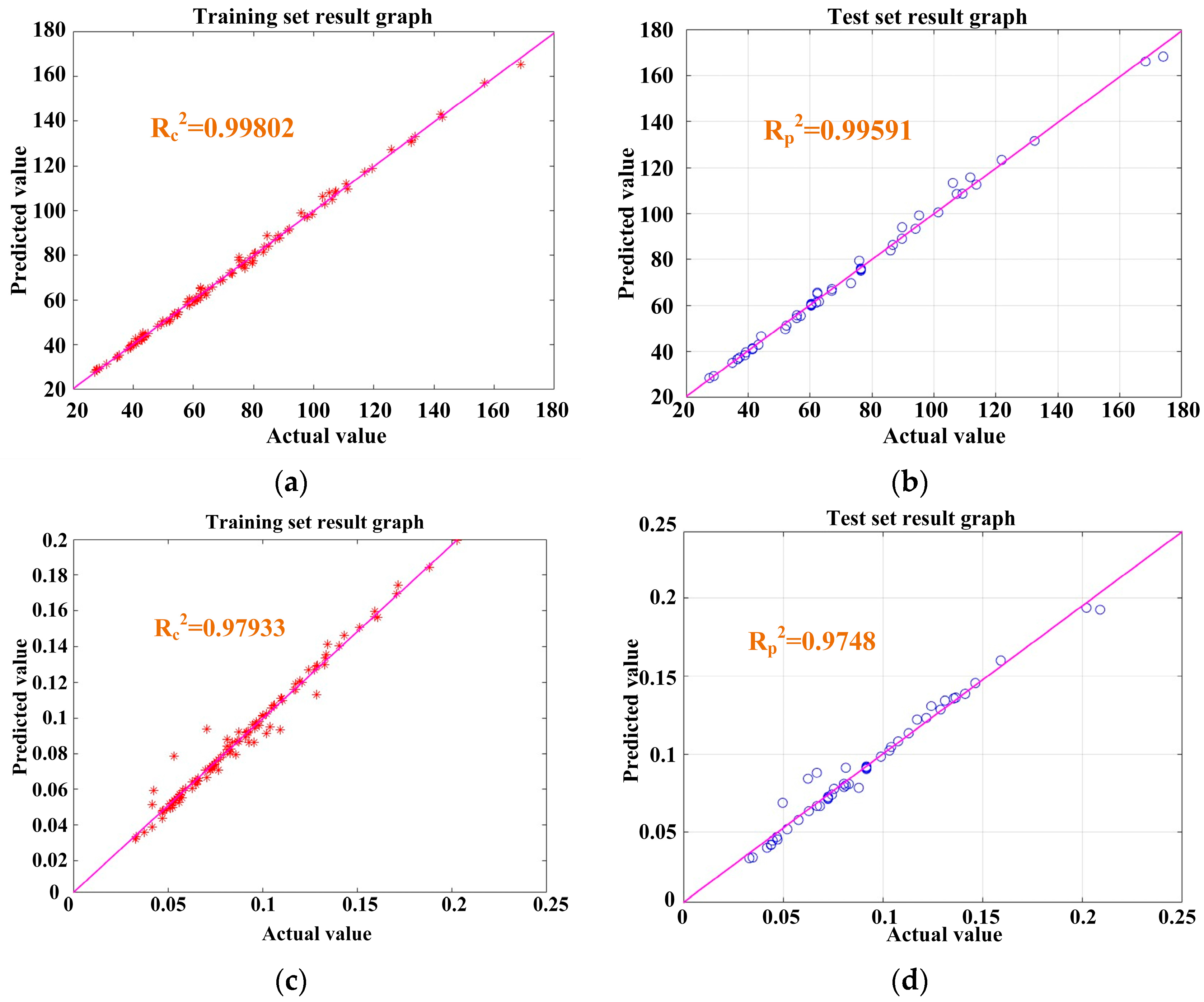
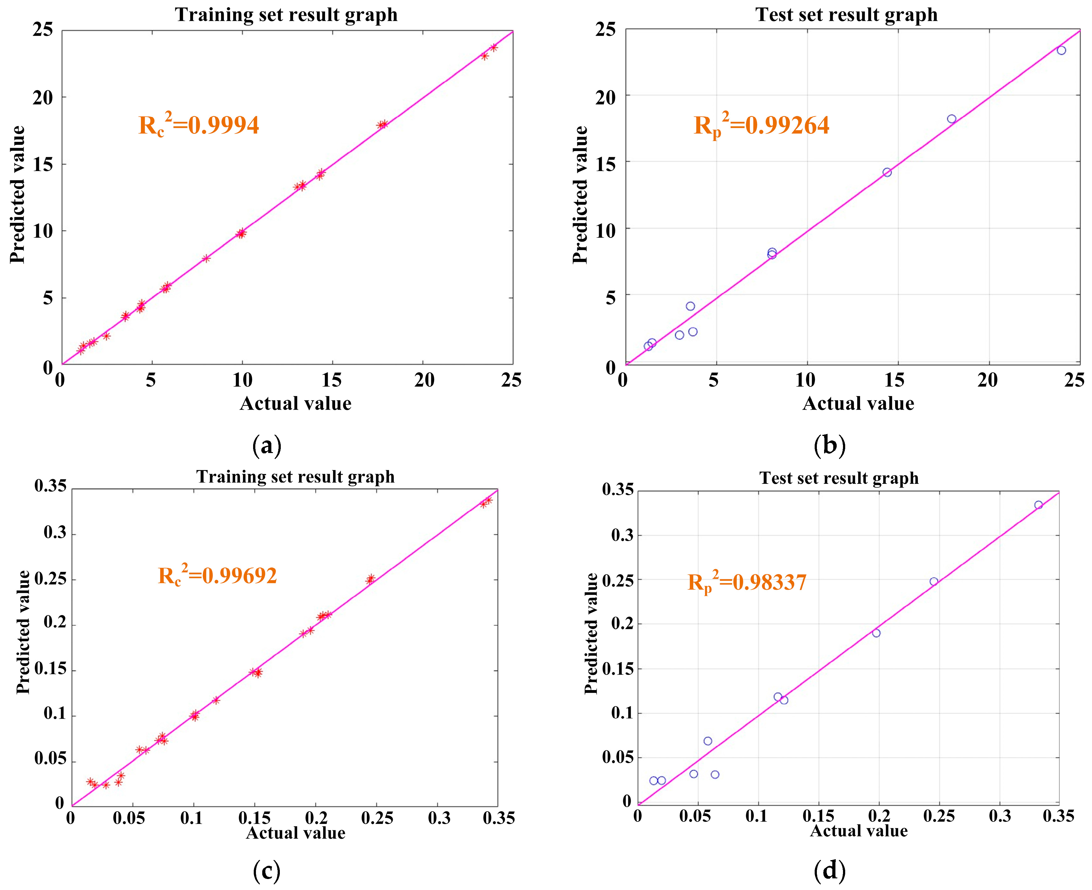
In Mode I, the following simulation conditions were established: flywheel speed of 3000 r/min; forward direction of the vehicle set in the x direction; speeds from 5 km/h to 20 km/h; and data trained using speed bumps on the above scale. Using the CNN+LSTM+ATTENTION, the PID parameters were trained and adjusted to meet the control requirements. Figure 8 shows graphs of the test set’s results and the training set’s results for parameters P and D. The results of the above three performance parameters are shown in Table 4, and it can be seen that good training results were achieved. It was applied to the flywheel system, and the simulation’s conditions were as follows: speed of 12 km/h; vehicle passed through two specifications of speed bumps, with a spacing of 2.6 m and with heights of 4 cm and 7 cm. It can be seen that the impact on the vehicle is divided into three stages: the vehicle’s front wheel make contact with the speed bumps; the front and rear wheels make contact with the speed bumps; and the rear wheel makes contact with the speed bumps, managed by the control system. The deflection of the flywheel under interference from the deceleration belt was obviously controlled. Figure 9 shows the axial z offset waveform under this working condition. During the whole process, the offset was kept within 0.025 mm under the interferences of the deceleration belts with different specifications.
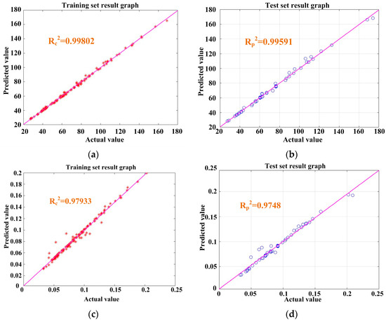
Figure 8.
Test set and training set diagrams for parameters P and D in Mode I: (a) parameter P, training set’s results; (b) parameter P, test set’s results; (c) parameter D, training set’s result; (d) parameter D, test set’s result. Where the purple line represents the actual value curve, the red asterisk represents the predicted value in the training set, and the blue circle represents the predicted value in the test set.
Table 4.
Evaluation parameters in Mode I.
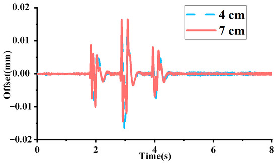
Figure 9.
Dynamic characteristics of the axial rotor of the flywheel in Mode I under the control of the parameters after training.
3.3. Mode II (Turning Mode)
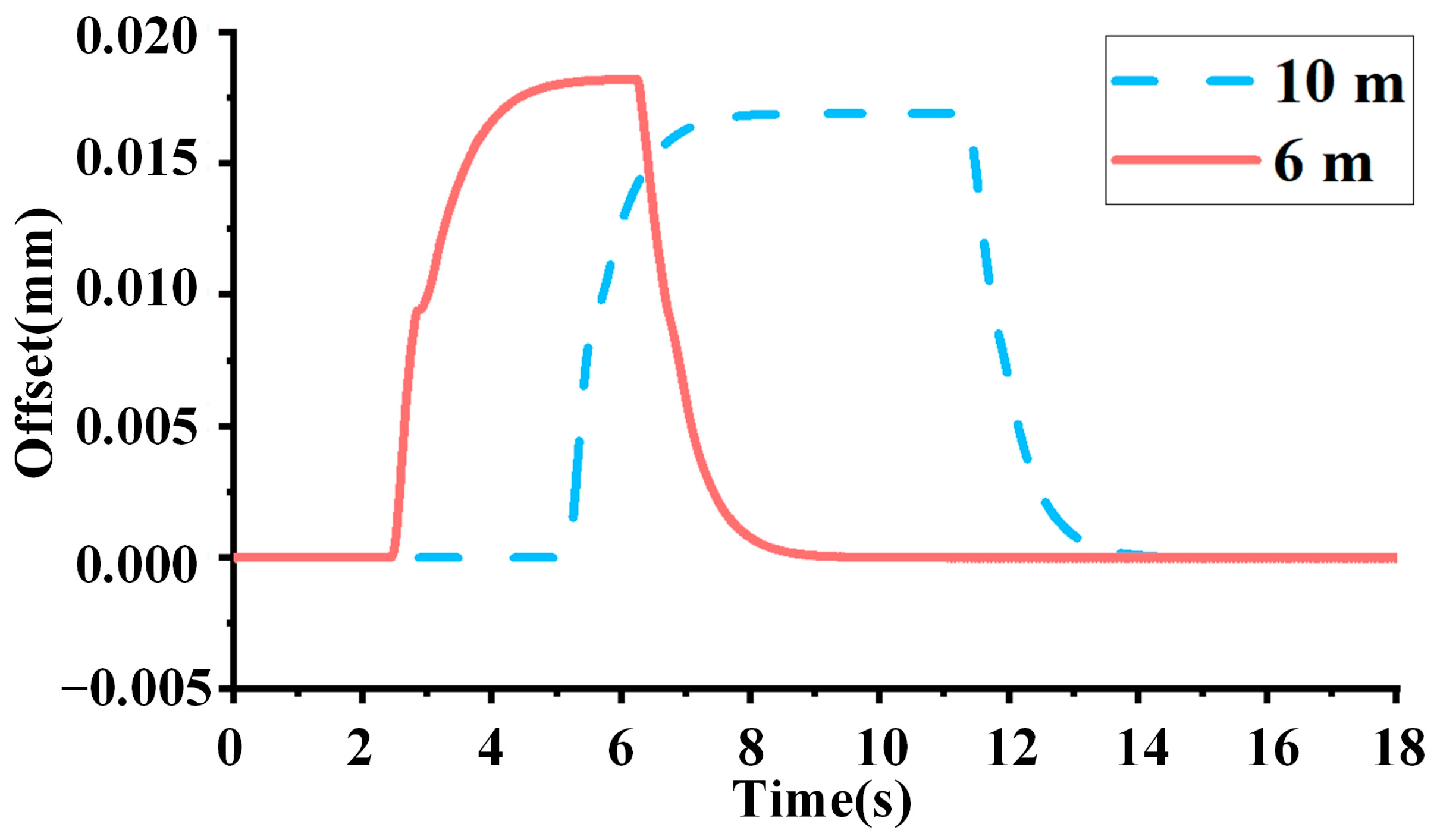
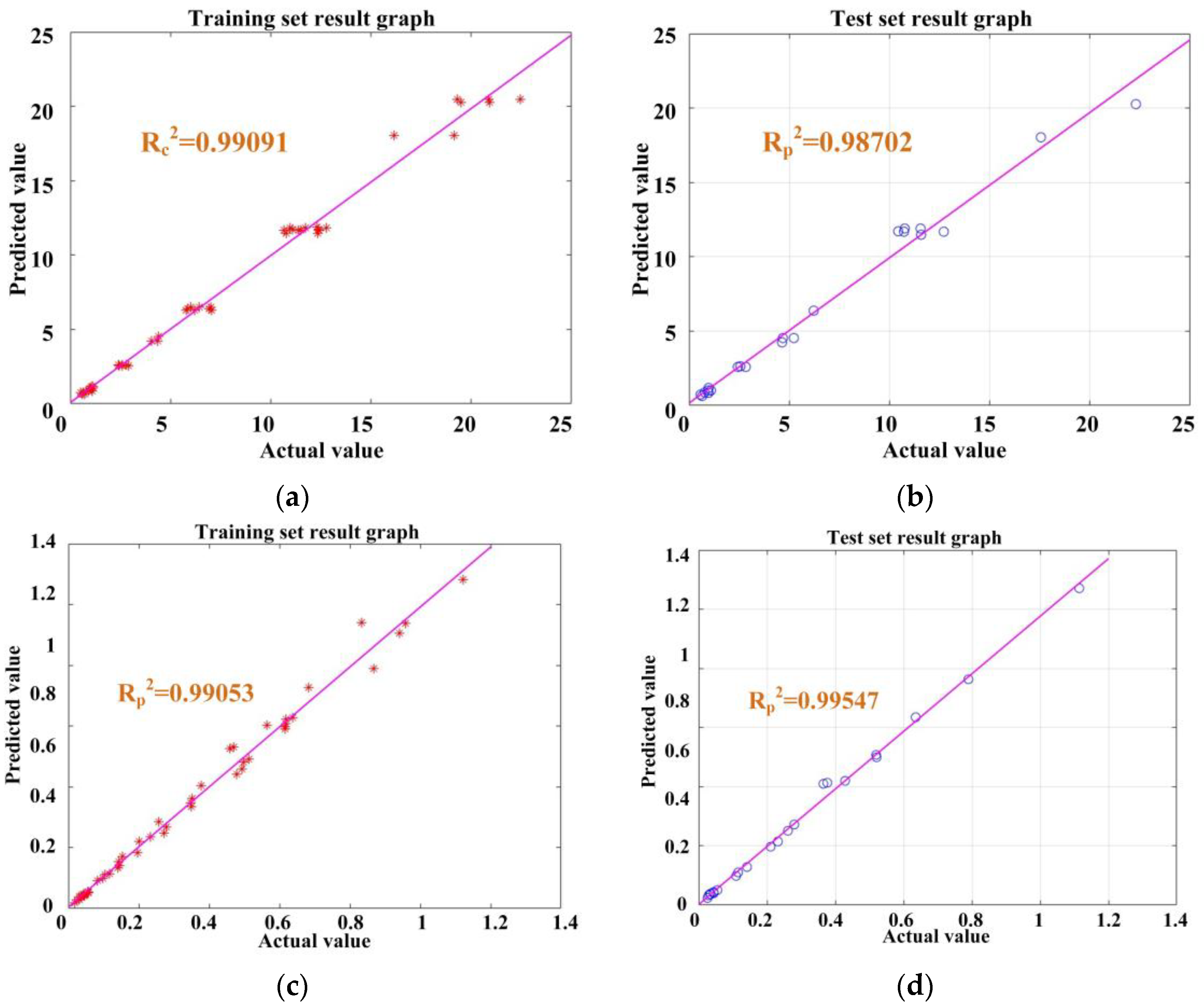
In Mode II, the simulation’s conditions were established as follows: flywheel speed of 3000 r/min; forward direction of the vehicle set in the x direction; speeds from 5 km/h to 20 km/h; and data are trained by the curves with turning radii of 6 m, 8 m, and 10 m. Through the CNN+LSTM+ATTENTION, the PID parameters were trained and adjusted to meet the control requirements. Figure 10 shows the test set and training set diagrams. The results of the above three performance parameters are shown below, and it can be seen that good training results were achieved. Applying it to the flywheel system, the simulation conditions were as follows: vehicle passed bends with turning radii of 10 m and 6 m at a speed of 24 km/h. It can clearly be seen that when the vehicle traveled on the bend, the interference it receives is a continuous process in the radial y direction. Under the management of the control system, the deflection of the flywheel under the interference from the deceleration belt was obviously controlled. Figure 11 shows the radial y offset waveform under this working condition. During the whole process, the offset was kept within 0.025 mm under the interference of that of different turning radii.
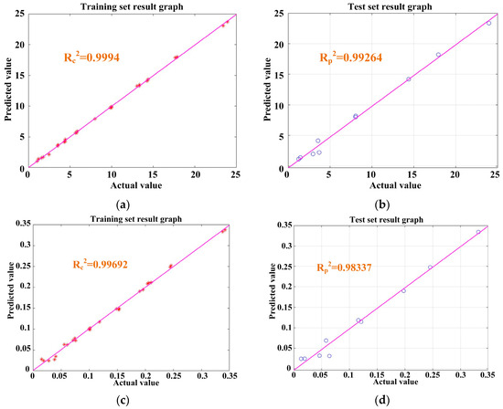
Figure 10.
Test set and training set diagrams for parameters P and D in Mode II: (a) parameter P, training set’s results; (b) parameter P, test set’s results; (c) parameter D, training set results; (d) parameter D, test set’s results. Where the purple line represents the actual value curve, the red asterisk represents the predicted value in the training set, and the blue circle represents the predicted value in the test set.
The results of the above three performance parameters are shown in Table 5.
Table 5.
Evaluation parameters in Mode II.
Table 5.
Evaluation parameters in Mode II.
| Evaluation Parameter | P | D |
|---|---|---|
| MAE | 0.44701 | 0.0094365 |
| MSE | 0.39894 | 0.0001673 |
| R2 | 0.99264 | 0.98337 |

Figure 11.
Dynamic characteristics of the radial rotor of the flywheel in Mode II under the control of the parameters after training.
Figure 11.
Dynamic characteristics of the radial rotor of the flywheel in Mode II under the control of the parameters after training.
3.4. Mode III (Uphill Mode)
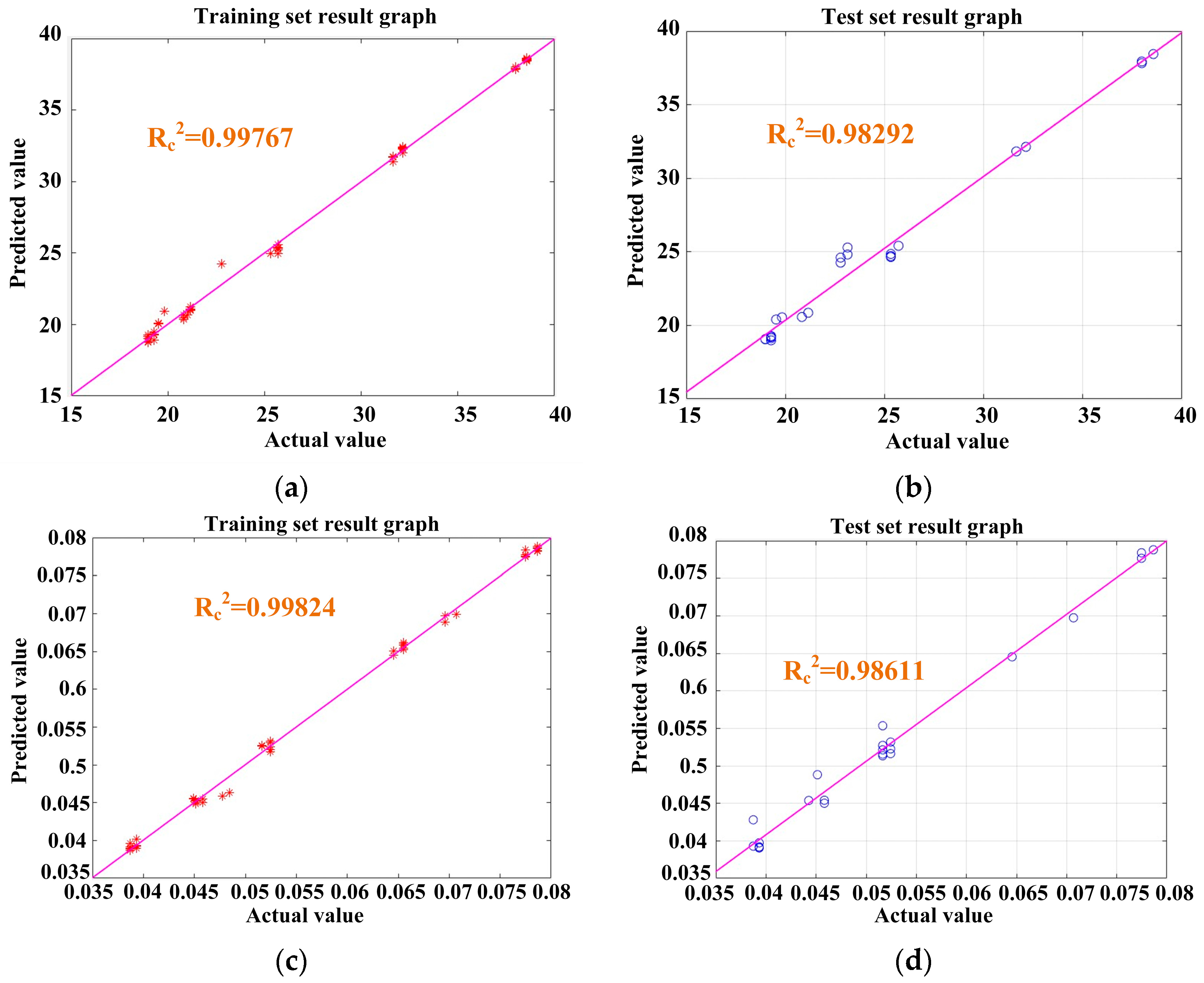
In Mode III, the simulation’s conditions were established as follows: flywheel speed of 3000 r/min; forward direction of the vehicle set in the x direction; speeds from 5 km/h to 20 km/h; and data trained on slopes of 10° and 20°. Using the CNN+LSTM+ATTENTION, the PID’s parameters were trained and adjusted to meet the control requirements. Figure 12 shows the test set and training set diagrams. The results of the above three performance parameters are shown below, and it can be seen that good training results were achieved. Applying it to the flywheel system, the simulation conditions were as follows: vehicle passed curves with a slope of 10° and 20° at a speed of 24 km/h. It can be clearly seen that when the vehicle passed the ramp, the interference it received was impact interference in the radial x direction and the axial z direction. Under the management of the control system, the deflection of the flywheel under interference from the deceleration belt was obviously controlled. Figure 13 shows the axial z offset waveform under this working condition. During the whole process, under interference from different slopes, the offset was kept within 0.025 mm.
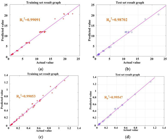
Figure 12.
Test set and training set diagrams for parameters P and D in Mode III: (a) parameter P, training set’s results; (b) parameter P, test set’s results; (c) parameter D, training set’s results; (d) parameter D, test set’s results. Where the purple line represents the actual value curve, the red asterisk represents the predicted value in the training set, and the blue circle represents the predicted value in the test set.
The results of the above three performance parameters are shown in Table 6.
Table 6.
Evaluation parameters in Mode III.
Table 6.
Evaluation parameters in Mode III.
| Evaluation Parameter | P | D |
|---|---|---|
| MAE | 0.45245 | 0.01369 |
| MSE | 0.4659 | 0.00035582 |
| R2 | 0.68257 | 0.99547 |
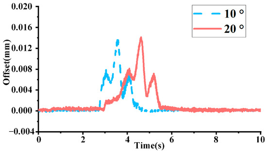
Figure 13.
Dynamic characteristics of the axial rotor of the flywheel in Mode III under the control of the parameters after training.
Figure 13.
Dynamic characteristics of the axial rotor of the flywheel in Mode III under the control of the parameters after training.

3.5. Mode IV (Encounters with Pedestrians Mode)
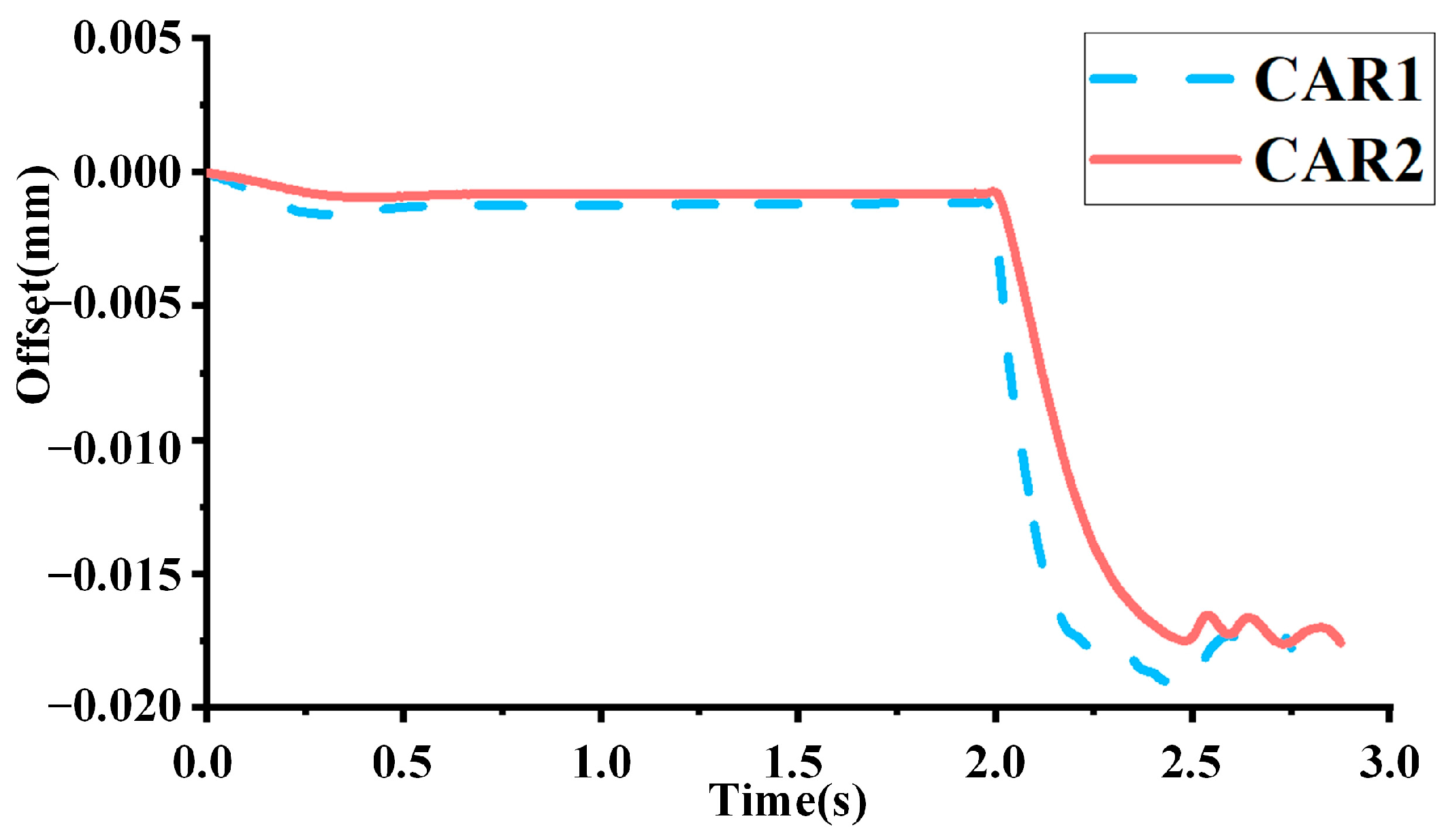
In Mode IV, the simulation’s conditions were established as follows: flywheel speed of 3000 r/min; forward direction of the vehicle set in the x direction; speeds from 5 km/h to 20 km/h; simulation of sudden encounters with pedestrians during normal, straight-line driving, applying emergency braking; and training the data. Using the CNN+LSTM+ATTENTION, the PID’s parameters were trained and adjusted to meet the control requirements. Figure 14 shows the test set and training set diagrams. The results of the above three performance parameters are shown below, and it can be seen that good training results were achieved. When it was applied to the flywheel system, the simulation conditions were as follows: CAR1 and CAR2 were run normally at a speed of 15 km/h, and emergency braking was performed after 2 s. It can clearly be seen that the different vehicles were subjected to different levels of interference during emergency braking, and the interference was impact interference in the radial x direction and axial z direction. Under the management of the control system, the deflection of the flywheel under the disturbance of the deceleration belt was obviously controlled. Figure 15 shows the offset waveform in the radial y direction under this working condition. During the whole process, the offset of the rotor was kept within 0.025 mm.
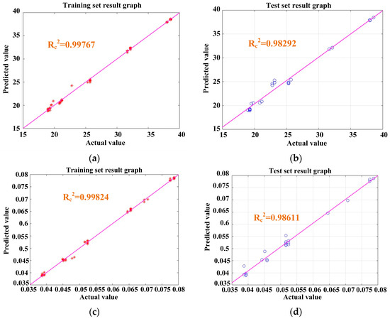
Figure 14.
Test set and training set diagrams for parameters P and D in Mode IV: (a) parameter P, training set results; (b) parameter P, test set’s result; (c) parameter D, training set results; (d) parameter D, test set’s result. Where the purple line represents the actual value curve, the red asterisk represents the predicted value in the training set, and the blue circle represents the predicted value in the test set.
The results of the above three performance parameters are shown in Table 7.
Table 7.
Evaluation parameters in Mode IV.
Table 7.
Evaluation parameters in Mode IV.
| Evaluation Parameter | P | D |
|---|---|---|
| MAE | 0.54159 | 0.0009255 |
| MSE | 0.6855 | 2.2303 × 10⁻⁶ |
| R2 | 0.98292 | 0.98611 |
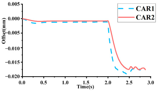
Figure 15.
Dynamic characteristics of the radial rotor of the flywheel in Mode IV under the control of the parameters after training.
Figure 15.
Dynamic characteristics of the radial rotor of the flywheel in Mode IV under the control of the parameters after training.
According to the above analysis, considering that typical working conditions (speed bumps, ramps, turns, and sudden pedestrians) have different interference intensities and directions for the flywheel, this manuscript used the SA-BPNN to determine the current working mode, taking into account speed bumps of different heights, ramps of different gradients, bends of different turning radii, and sudden appearance of pedestrians while driving at different speeds. All of them have different degrees of impact on the flywheel. Therefore, using the CNN+LSTM+ATTENTION and the characteristics of the neural network, the accuracy and generalization ability of the model can be improved in terms of performance, and the parameters of the PID controller under different working conditions were trained so that the PID’s control parameters could be applied to different working conditions and road specifications. The results show that the trained control parameters met the stability requirements (the rotor offset was less than 0.025 mm).
When extended to flywheel systems with different rotation masses, materials, shapes, and motors, the corresponding interference data under complex conditions exhibited high diversity. For example, under different working conditions, such as operating temperature, load change, and speed range, the interference data generated by different flywheels will be very different. We need to re-simulate these interference data, and after the simulation, we also need to train using these re-simulated data to ensure that the control strategy can achieve the ideal control effect in the face of different types of flywheels. Therefore, it is necessary to establish different flywheel models in SolidWorks, import them into ADAMS/VIEW2020 for assembly, co-simulate the flywheel built in ADAMS/VIEW2020 with ADAMS/CAR2020, obtain the corresponding control parameters under complex conditions, and then retrain them before they can be used in the existing flywheel system. Moreover, related content can be added to the text for yellow processing. In order for experts to more clearly understand the impacts of factors such as rotation quality on the flywheel control system, we explain this in more detail.
In a flywheel, the rotation quality, material, shape, and motor are different, and the control effect will be different. The rotational mass is large, the moment of inertia is large, and the system’s response is slow but more stable. The material’s characteristics are different; high-strength materials can withstand the high-speed storage of more energy. The magnetic properties of the material affect the efficiency and torque of the motor and, thus, affect the control effect. In terms of shape, the moment of inertia’s distributions for different shapes of flywheels are different, such as the moment of inertia of a hollow cylinder flywheel being related to the outside diameter, inside diameter, and height, and the change in angular speed is also different when the torque interferes. There are many types of motors; for example, brushless DC motors rely on the control system to precisely control the current, break, and direction; otherwise, torque fluctuations affect the flywheel, and the speed and torque control accuracy requirements are high. The PM synchronous motor requires the control system to accurately adjust the three-phase AC and adapt to different working states to maintain high efficiency, and the high-precision control requirements increase the algorithm’s complexity. The asynchronous characteristics of induction motors require the control system to adapt to speed differences. Complex speed regulation technology requires a high computing power and algorithm optimization, and efficiency problems affect the overall efficiency of the system. The control systems of reluctance motors must control the current according to its characteristics, and special strategies are needed to make up for the lack of torque density, relying on the rotor position information to control the current. Various combinations of these factors lead to different control effects on the flywheel. Therefore, the control parameters should be modified according to different factors such as the flywheel material.
4. Experiments and Results
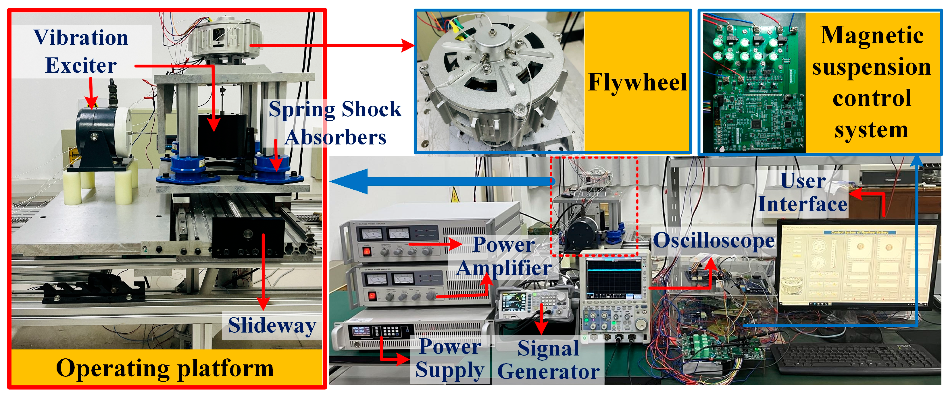
In order to verify the superiority of the designed control system in suppressing the interference from vehicle-driving conditions, the robustness of the flywheel is tested on the experimental platform. As shown in Figure 16, the whole platform mainly includes vehicle flywheel, operating platform simulating various vehicle-driving conditions and magnetic levitation control system. The operating platform simulating various vehicle-driving conditions adopts modular design, which can carry out experiments on single vehicle-driving conditions, automobile suspension, road conditions, etc., and can also carry out multifactor comprehensive experiments. The module used in this paper has a three-dimensional slipway platform (x, y, z axis three degrees of freedom), which can simulate the vehicle acceleration and deceleration, uphill and downhill, turning and other working conditions. In addition, this paper also uses the x, y direction of the exciter and other components, with three-dimensional slide, to simulate the high-speed vehicle acceleration, turning, uphill and downhill conditions.
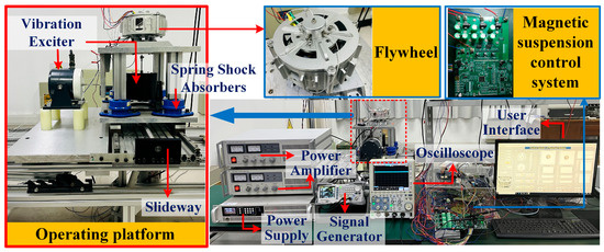
Figure 16.
Overall experimental platform.
Figure 16 is the overall experimental platform, which includes a flywheel prototype, a magnetic suspension control system, and an operating platform for imitating automobile suspension, driving conditions, and road conditions, on which flywheel is installed. The automobile suspension system is imitated by four spring shock absorbers, while road conditions were imitated by the function signal generator and vibration exciters. The left vibration exciter was used to imitate the driving conditions. In addition, the road function can be programmed through the signal generator to drive the correct shaker to simulate the road. Then, the force sensor is used to judge the strength of the interference signal.
Based on the experimental platform shown in Figure 16, the performance test of the control system was carried out, and the comparative experiment using the classical PID control system was added.
In this experiment, mode IV was selected as the experimental condition of the above four working modes to test the stability of the flywheel rotor under the action of the control system in this working mode. In this experiment, the impact interference with the flywheel was simulated when the vehicle encountered a pedestrian at low speed and braking. The flywheel operated in a stable state until a pedestrian was encountered. The experimental conditions were as follows: flywheel rotor speed of 3000 r/min; to ensure the experimental platform was driven in a straight line at a speed of 1.4 m/s, the forward direction was located in the x direction of the flywheel rotor; and emergency braking occurred after 1.5 s. The bias of the flywheel accumulator rotor and the control effect of the system are observed and obtained.
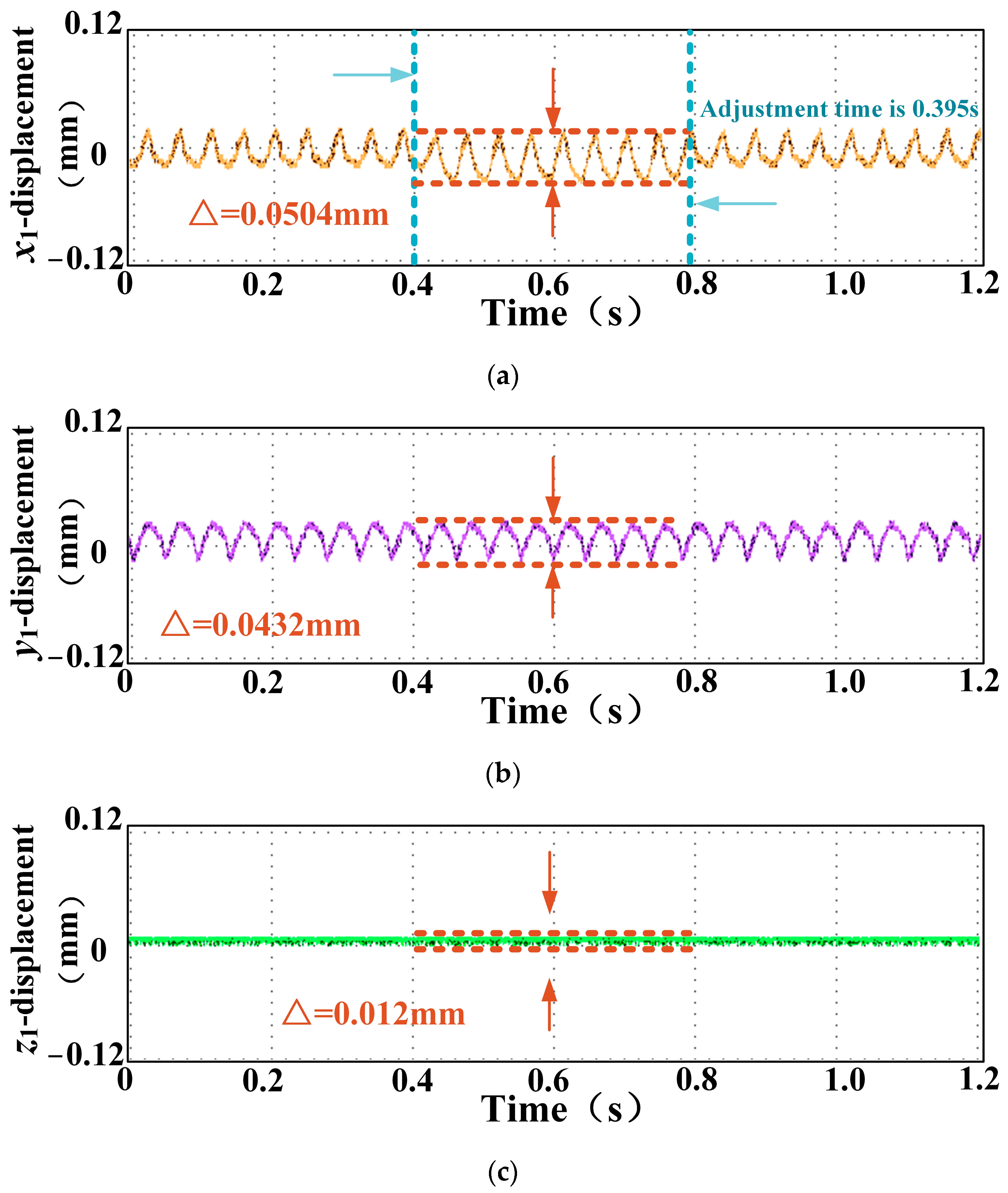
The deflection waveform of the flywheel rotor under the impact of the sudden pedestrian encounter control strategy proposed in this paper is shown in Figure 17. When the vehicle encounters a pedestrian, it applies emergency braking, and the flywheel will be severely impacted by this braking. The experimental platform encountered a pedestrian at 0.4 s; there was a lag in the radial x1 direction, the peak-to-peak offset value was 0.0504 mm, and the whole process lasted 0.395 s. In the radial y1 direction, the mean peak-to-peak value was almost constant at 0.0432 mm. From an axial point of view, because of the low speed and the flywheel being in a stable state of operation, the interference with the shaft disappeared during the startup, and the prototype’s own structure can offset the interference with the shaft when it encounters a pedestrian.
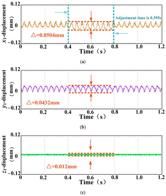
Figure 17.
The dynamic performance of the flywheel based on the SA-BPNN and CNN+LSTM+ATTENTION control strategy: (a) displacement in the x1 direction; (b) displacement in the y1 direction; (c) displacement in the z1 direction. Where the blue dashed line indicates the area where the road condition occurs and ends, and the blue arrow indicates the adjustment time. The brown dashed lines represent the maximum and minimum areas of the waveform, and the brown arrows represent the peak-to-peak values of the waveform.
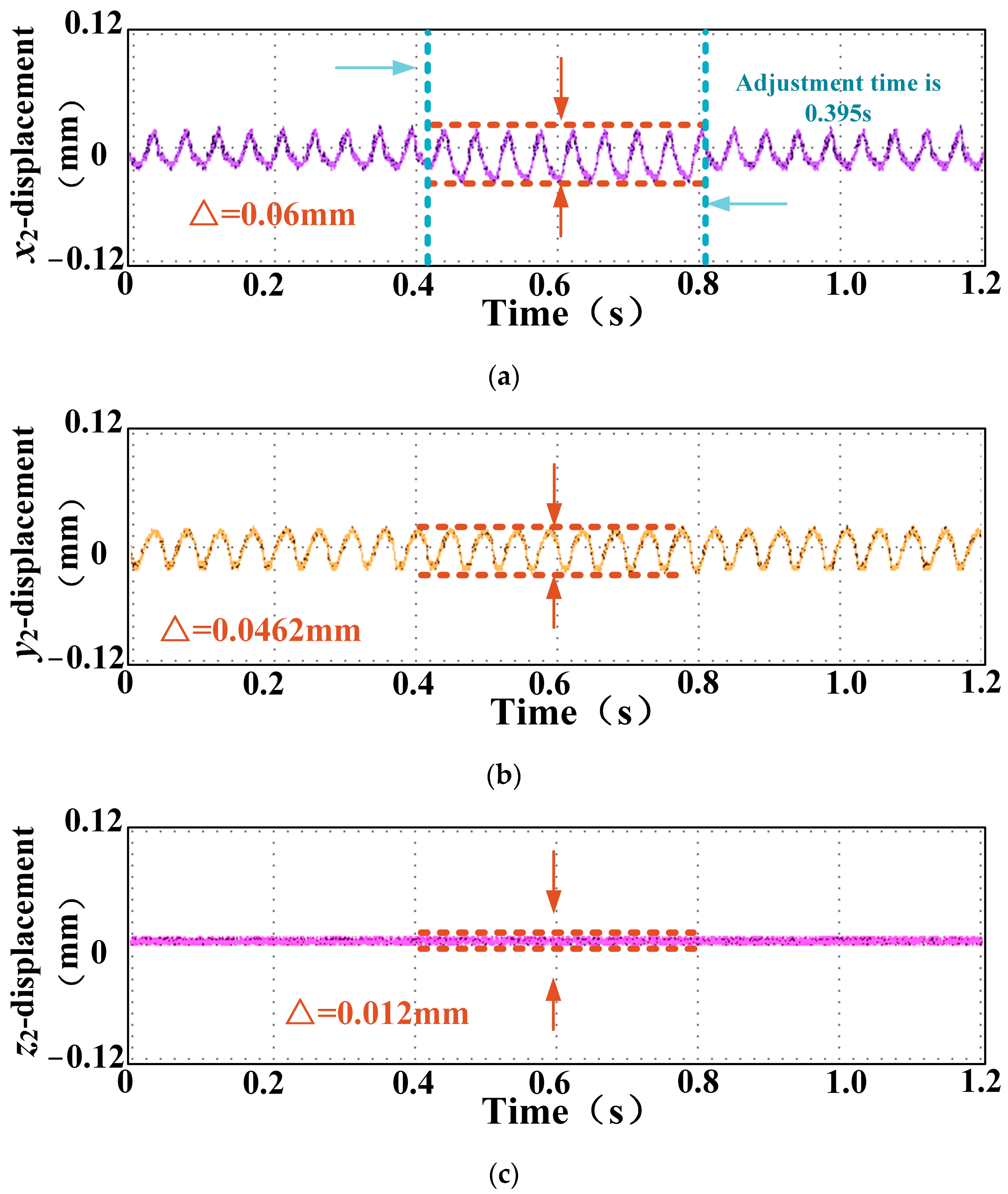
The deflection waveform of a flywheel rotor under the impact of sudden pedestrian encounters controlled by a conventional PID is shown in Figure 18. The experimental platform encountered pedestrians at 0.42 s, and there was a lag in the radial x2 direction, the peak-to-peak offset value was 0.06 mm, and the whole process lasted 0.395 s. In the radial y2 direction, the mean peak-to-peak value was almost constant at 0.0462 mm. The axial direction did not change because of the structural characteristics of the flywheel itself. According to the comparison of the above two experimental results, it is obvious that the control strategy proposed in this paper is superior to the traditional PID control strategy in terms of stability under the same working conditions.
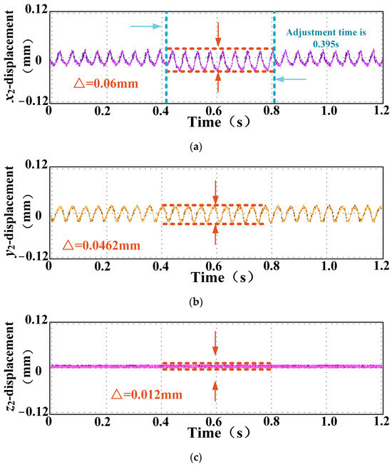
Figure 18.
The dynamic performance of the flywheel when encountering pedestrians is controlled based on the classical PID: (a) displacement in the x2 direction; (b) displacement in the y2 direction; (c) displacement in the z2 direction. Where the blue dashed line indicates the area where the road condition occurs and ends, and the blue arrow indicates the adjustment time. The brown dashed lines represent the maximum and minimum areas of the waveform, and the brown arrows represent the peak-to-peak values of the waveform.
5. Conclusions
Traditional methods often ignore the direct influences of various working conditions on flywheel systems, as well as the influence of low-precision control parameter adjustments on the stability of the flywheel. A flywheel control strategy with high stability based on the SA-BPNN and CNN+LSTM+ATTENTION was proposed in this manuscript. Compared with a traditional PID control strategy, the neural network can be used to train different road conditions and vehicle speed data under different working conditions, cooperating with the working mode recognition to improve the accuracy and stability of the control system and improve the response speed under typical working conditions. The experimental results show that the stability of the flywheel system obviously improved under complex conditions.
In addition, it is worth noting that the method proposed in this manuscript is universal. When training the model in this manuscript, the interference of different working conditions on the flywheel under classical working conditions is taken into account. The common road condition specifications under the current working conditions (speed bumps with a height of 4 cm, curves with a turning radius of 6 m, ramps with slopes of 10°, etc.), and vehicle speeds (5 km/h, 10 km/h, etc.) were selected to establish the relationships between different working conditions and control parameters. If road condition specifications and vehicle speeds not considered in the training model are encountered, the PID control parameters suitable for the current road conditions can be determined using the above model. For flywheels with different rotation masses, materials, shapes, and motors, merely changing the parameters of the data set required for training can result in accurate working condition judgments and stability control.
As this paper only selected representative cases of four common working conditions in daily life for analysis, under actual complex working conditions, the differences among working conditions, situations of different vehicle-mounted flywheels, and the impacts of different traffic conditions on flywheels need to be further discussed, and better algorithms can be developed to improve the control accuracy. The flywheel can also maintain stable operation under more complex conditions.
Author Contributions
Project administration, W.Z.; Writing—original draft, W.Z. and H.J.; Conceptualization, W.Z.; methodology, H.J.; software, H.J.; validation, H.J. All authors have read and agreed to the published version of the manuscript.
Funding
This work was supported in part by the National Natural Science Foundation of China, under grant 52077099, and in part by the Project Funded by the Priority Academic Program Development of Jiangsu Higher Education Institutions.
Data Availability Statement
No new data were created or analyzed in this study. Data sharing is not applicable to this article.
Conflicts of Interest
The authors declare no conflicts of interest.
References
- Bianchini, C.; Torreggiani, A.; David, D.; Bellini, A. Design of motor/generator for flywheel batteries. IEEE Trans. Ind. Electron. 2021, 68, 9675–9684. [Google Scholar] [CrossRef]
- Mehrjardi, R.T.; Ershad, N.F.; Ehsani, M. Transmotor-flywheel powertrain assisted by ultracapacitor. IEEE Trans. Transp. Electrif. 2022, 8, 3686–3695. [Google Scholar] [CrossRef]
- Hou, J.; Song, Z.; Hofmann, H.F.; Sun, J. Control strategy for battery/flywheel hybrid energy storage in electric shipboard microgrids. IEEE Trans. Ind. Inform. 2021, 17, 1089–1099. [Google Scholar] [CrossRef]
- Kermani, M.; Shirdare, E.; Parise, G.; Bongiorno, M.; Martirano, L. A comprehensive technoeconomic solution for demand control in Ports: Energy Storage Systems Integration. IEEE Trans. Ind. Appl. 2022, 58, 1592–1601. [Google Scholar] [CrossRef]
- Li, Y.; Ding, Z.; Yu, Y.; Liu, Y. Coordinated Control of Engine-Load-Storage for Marine Micro Gas Turbine Power Generation System. In The Proceedings of 2023 International Conference on Wireless Power Transfer (ICWPT2023). ICWPT 2023; Lecture Notes in Electrical Engineering; Cai, C., Qu, X., Mai, R., Zhang, P., Chai, W., Wu, S., Eds.; Springer: Singapore, 2024; Volume 1160. [Google Scholar]
- McGroarty, J.; Schmeller, J.; Hockney, R.; Polimeno, M. Flywheel energy storage system for electric start and an all-electric ship. In Proceedings of the IEEE Electric Ship Technologies Symposium, Philadelphia, PA, USA, 25–27 July 2005; pp. 400–406. [Google Scholar]
- Cao, Z.; Tao, J.; Ma, T.; Zeng, X.; Yu, M. Adaptive inertial control of marine energy storage for pulsed power load. In Proceedings of the 2024 IEEE 7th International Electrical and Energy Conference (CIEEC), Harbin, China, 10–12 May 2024; pp. 4686–4691. [Google Scholar]
- Alahakoon, S.; Leksell, M. Emerging energy storage solutions for transportation—A review: An insight into road, rail, sea and air transportation applications. In Proceedings of the 2015 International Conference on Electrical Systems for Aircraft, Railway, Ship Propulsion and Road Vehicles (ESARS), Aachen, Germany, 3–5 March 2015; pp. 1–6. [Google Scholar]
- Hou, J.; Sun, J.; Hofmann, H. Battery/flywheel Hybrid Energy Storage to mitigate load fluctuations in electric ship propulsion systems. In Proceedings of the 2017 American Control Conference (ACC), Seattle, WA, USA, 24–26 May 2017; pp. 1296–1301. [Google Scholar]
- Soni, T.; Sodhi, R. Impact of harmonic road disturbances on active magnetic bearing supported flywheel energy storage system in electric vehicles. In Proceedings of the IEEE International Transportation Electrification Conference (ITEC), Bengaluru, India, 17–19 December 2019; pp. 1–4. [Google Scholar]
- Numanoy, N.; Srisertpol, J. Vibration reduction of an overhung rotor supported by an active magnetic bearing using a decoupling control system. Machines 2019, 7, 73. [Google Scholar] [CrossRef]
- Mehraban, A.; Farjah, E.; Ghanbari, T.; Garbuio, L. Integrated optimal energy management and sizing of hybrid battery/flywheel energy storage for electric vehicles. IEEE Trans. Ind. Inform. 2023, 19, 10967–10976. [Google Scholar] [CrossRef]
- Han, B.; Chen, Y.; Li, M.; Zheng, S.; Zhang, X. Stable control of nutation and precession for the radial four-degree-of-freedom AMB-rotor system considering strong gyroscopic effects. IEEE Trans. Ind. Electron. 2021, 68, 11369–11378. [Google Scholar] [CrossRef]
- Wang, J.G.; Su, J.H.; Lai, J.D.; Zhang, J.; Wang, S.Y. Research on control method for flywheel energy storage system. In Proceedings of the 2016 IEEE 8th International Power Electronics and Motion Control Conference, Hefei, China, 22–26 May 2016; pp. 1006–1010. [Google Scholar]
- Jaafar, A.; Akli, C.R.; Sareni, B.; Roboam, X.; Jeunesse, A. Sizing and energy management of a hybrid locomotive based on flywheel and Accumulators. IEEE Trans. Veh. Technol. 2009, 58, 3947–3958. [Google Scholar] [CrossRef]
- Wu, C.; Xu, B.; Lu, S.; Xue, F.; Jiang, L.; Chen, M. Adaptive eco-driving strategy and feasibility analysis for electric trains with onboard energy storage devices. IEEE Trans. Transp. Electrif. 2021, 7, 1834–1848. [Google Scholar]
- Chen, Q.; Liu, G.; Han, B. Suppression of imbalance vibration in AMB-rotor systems using adaptive frequency estimator. IEEE Trans. Ind. Electron. 2015, 62, 7696–7705. [Google Scholar] [CrossRef]
- Cui, P.; Wang, Q.; Zhang, G.; Gao, Q. Hybrid fractional repetitive control for magnetically suspended rotor systems. IEEE Trans. Ind. Electron. 2018, 65, 3491–3498. [Google Scholar] [CrossRef]
- Zhang, W.; Zhu, P.; Wang, J.; Zhu, H. Stability control for a centripetal force type-magnetic bearing-rotor system based on golden frequency section Point. IEEE Trans. Ind. Electron. 2021, 68, 12482–12492. [Google Scholar] [CrossRef]
- Zhang, W.; Cheng, L.; Zhu, H. Suspension force error source analysis and multidimensional dynamic model for a centripetal force type-magnetic bearing. IEEE Trans. Ind. Electron. 2020, 67, 7617–7628. [Google Scholar] [CrossRef]
- Zhang, W.; Yang, H.; Cheng, L.; Zhu, H. Modeling based on exact segmentation of magnetic field for a centripetal force type-magnetic bearing. IEEE Trans. Ind. Electron. 2020, 67, 7691–7701. [Google Scholar] [CrossRef]
- Ding, G.; Zhou, Z.; Hu, Y. Test of base vibration influence on dynamics of a magnetic suspended disk. In Proceedings of the 2008 IEEE/ASME International Conference on Advanced Intelligent Mechatronics (AIM), Xi’an, China, 2–5 July 2008; pp. 308–313. [Google Scholar]
- Zhang, W.; Zhang, L.; Li, K.; Zhu, H. Dynamic correction model considering influence of foundation motions for a centripetal force type-magnetic bearing. IEEE Trans. Ind. Electron. 2021, 68, 9811–9821. [Google Scholar] [CrossRef]
- Zhang, W.; Wang, Z. Dual mode coordinated control of magnetic suspension flywheel based on vehicle driving conditions characteristics. IEEE Trans. Transp. Electrif. 2024, 10, 2124–2134. [Google Scholar] [CrossRef]
- Zhang, W.; Wang, J.; Zhu, P.; Yu, J. A novel vehicle-mounted magnetic suspension flywheel with a virtual inertia spindle. IEEE Trans. Ind. Electron. 2022, 69, 5973–5983. [Google Scholar] [CrossRef]
- Zhang, W.Y.; Cui, J.J. Dynamic performance analysis and control parameter adjustment algorithm for flywheel batteries considering vehicle direct action. Energies 2023, 16, 5882. [Google Scholar] [CrossRef]
- Zhu, Z.; Qi, G.; Xu, J.; Li, X. Dynamic modeling of the support system for vehicle-mounted spherical magnetic suspension flywheel. IEEE Trans. Energy Convers. 2024, 39, 322–333. [Google Scholar] [CrossRef]
- Zhang, W.; Wang, J.; Li, A.; Xiang, Q. Multiphysics fields analysis and optim-ization design of a novel saucer-shaped magnetic suspension flywheel battery. IEEE Trans. Transp. Electrific. 2024, 10, 5473–5483. [Google Scholar] [CrossRef]
- Zhao, H.; Liu, M.; Sun, Y.; Chen, Z.; Duan, G.; Cao, X. Automated design of fault diagnosis CNN network for satellite attitude control systems. IEEE Trans. Cybern. 2024, 54, 4028–4038. [Google Scholar] [CrossRef] [PubMed]
- Wang, S.; Zhu, H.; Wu, M.; Zhang, W. Active disturbance rejection decoupling control for three-degree-of- freedom six-pole active magnetic bearing based on BP neural network. IEEE Trans. Appl. Supercond. 2020, 30, 3603505. [Google Scholar] [CrossRef]
- Syed, A.; Mufti, M.U.D. Neural Networks based Adaptive Predictive Control of Flywheel Energy Storage for Hybrid Power Systems. In Proceedings of the 2023 IEEE International Conference on Power Electronics, Smart Grid, and Renewable Energy (PESGRE), Trivandrum, India, 17–20 December 2023; pp. 1–6. [Google Scholar]

Disclaimer/Publisher’s Note: The statements, opinions and data contained in all publications are solely those of the individual author(s) and contributor(s) and not of MDPI and/or the editor(s). MDPI and/or the editor(s) disclaim responsibility for any injury to people or property resulting from any ideas, methods, instructions or products referred to in the content. |
© 2024 by the authors. Licensee MDPI, Basel, Switzerland. This article is an open access article distributed under the terms and conditions of the Creative Commons Attribution (CC BY) license (https://creativecommons.org/licenses/by/4.0/).