Abstract
This article analyzes the factors causing the precision error of the robot joint module, such as gear meshing disturbance, output elastic deformation, and load mutation. An improved active disturbance rejection control (ADRC) algorithm is proposed to overcome the uncertainty of nonlinear factors and variables of this research topic. The output precision loss of the joint module is introduced as a new input variable of ADRC, combined with the input variable of torque current of the joint module. The extended state observer is redesigned, and the online estimation of disturbance is realized. According to the disturbance estimation results, the current loop algorithm of permanent magnet synchronous motors is improved to compensate the torque disturbance of the robot joint module. The experimental results show that the improved ADRC algorithm can obviously suppress the disturbance of the joint module, weaken the meshing error and torque output deformation of the harmonic reducer gear, and improve the control accuracy of the joint module.
1. Introduction
In recent years, active disturbance rejection control (ADRC) has been widely used in the control of permanent magnet synchronous motors such as the pure electric drive for electric vehicles, industrial servos, and the drive for mechanical hard disk servo motors. After nearly 20 years of development, ADRC has put forward the idea of disturbance compensation from theoretical research to practical application and has achieved broad development. Compared with traditional proportional-integral-derivative (PID) control and sliding mode control, active disturbance rejection control exhibits stronger disturbance rejection ability and higher robustness, which can better solve the contradiction between speed and stability. Due to the diversity of application industries, complexity of operating conditions, and uncertainty of disturbance variables in motor control systems, scholars have conducted extensive and in-depth explorations of ADRC, mainly focusing on the following aspects: (1) Improving the design and parameter tuning of a linear extended state observer (LESO) while ensuring system convergence and algorithm efficiency. Dr. Gao proposed the linearization of the error feedback function, which is the most typical improvement method [1]. (2) Enhancing the disturbance resistance of ADRC, scholars proposed the concept of a high-order extended state observer (ESO) (generalized extended state observer, GESO), which designs multiple extended states for GESO. When the m-order derivative of the total disturbance is zero, GESO can ensure convergence. (3) Reducing the observation burden of ESO, convergence speed is improved and known disturbances in the system are separated from the total disturbances, which ensures that ESO only observes unknown disturbances, and thus the robustness of the system is enhanced.
With the development of the robotics industry, ADRC technology also found some applications in the robotics industry such as the following: (1) In robot control, active disturbance rejection control is used to solve the trajectory tracking problem of robots. For example, in the control of omnidirectional mobile robots, a dynamic controller based on backstepping and an improved extended state observer is designed to cope with unknown disturbance phenomena [2]. (2) ADRC resolves the balance issue in robot control. Reference [3] focuses on the dynamic models of robots with multiple variables and strong coupling. By using the active disturbance rejection control method and introducing virtual control variables, decoupling control is achieved to stabilize the balance of the robot. (3) In the research on improving the control accuracy of robots, Ref. [4] proposed a kinematic model and a joint position sensitive error model based on an improved Denavit Hartenberg (MD-H) model to enhance the pose accuracy of industrial robots. Ref. [5] proposed an improved gray wolf algorithm to optimize the motion accuracy of robots. By transforming the robot accuracy problem into a nonlinear system optimization problem through a model, the optimal parameters of the robot were obtained to improve the control accuracy of the robot. To improve the accuracy of harmonic reducers, Ref. [6] redesigned a harmonic gear reducer based on the physical requirements of gears and the characteristics of robot technology and verified parameters such as gear accuracy, strength, and safety factors. Ref. [7] designed an involute harmonic reducer gear to minimize tooth tip interference. Design parameters such as pressure angle, tooth height, profile offset coefficient, and number of teeth were simulated to improve the accuracy performance of robot joint actuators.
In the research and active disturbance rejection control of robots, the focus is mainly on the control of the robot body, while there is relatively little research on the robot joints. Currently, the highest positioning accuracy of joint module is 15 arcseconds. This accuracy depends on the accuracy of the harmonic reducer itself. This article will use an ADRC algorithm to improve the control accuracy of the robot joint module. The main contributions are as follows:
- (1)
- The current measures to improve the accuracy of robots are either focused on compensating the dynamic model and optimizing the parameters of robots, or on improving the accuracy of harmonic reducers from a mechanical design perspective. The design of control theory and harmonic reducers has not been well integrated in the current research. This article incorporates the advantages of two types of precision improvement and combines control theory with the characteristics of harmonic reducers to systematically study robot joints. A precision compensation technology for robot joint modules is proposed.
- (2)
- This article expands the research topic of ADRC and studies the harmonic reducer and the PMSM as a whole control object. In robot motion control, traditional ADRC studies the dynamic performance, steady-state accuracy, and disturbance rejection ability of the PMSM output shaft. In fact, the motion angle output of the motor is converted by the harmonic reducer to obtain the motion angle of the robot. During this angle conversion process, there are important factors that affect the accuracy of robot motion, such as gear deformation, load disturbance, and mechanical vibration. Even if the PMSM achieves precise control of motor output, the accuracy transmitted to the end of the robot is greatly reduced, which is also the difficulty of robot accuracy control. This article adopts a new approach, which differs from the traditional approach of only controlling the output shaft accuracy of the PMSM. The harmonic reducer model is integrated into the PMSM control strategy to redesign the ADRC controller. By adjusting the output of the ADRC torque loop to counteract these uncertain torque disturbances, the control accuracy can be improved.
2. Mathematical Model of Robot Joint Module
2.1. PMSM-Harmonic Reducer System
In the research and development of robots, the joint module is an important part of the robot structure. It integrates the core components of the robot such as permanent magnet synchronous motor (PMSM), harmonic reducer, sensor and servo drive for joint movement and position control of the robot. The control performance of the joint module directly affects the motion precision, speed, and stability of the robot.
As shown in Figure 1, the robot integrated joint module is mainly composed of the harmonic reducer, PMSM, brake, encoder, drive controller, etc. A high-speed encoder and low-speed encoder are, respectively, installed on the motor bearing of the joint module and the output bearing of the reducer, which are used to obtain the real-time position of the motor and the harmonic reducer. The servo drive uses a vector control algorithm to accurately track the PMSM position and torque. After the output of the servo motor is amplified by the harmonic reducer, the position of higher precision and higher torque is obtained. At present, the popular control strategy mainly adopts a three-loop control strategy of torque, speed, and position to control the position output of the robot joint module. The difference between the position command is calculated to obtain the operating angle of the synchronous motor, and the first derivative of the position command is calculated to obtain the operating speed of the synchronous motor. In this sense, it mainly controls the motor position of the permanent magnet synchronous motor harmonic reducer system, i.e., it controls the position of the high-speed end encoder. The low-speed encoder of the harmonic reducer is mainly used for a multi turn position calculation of the robot and sends these data to the robot controller to ensure that the robot operates within a fixed angle range and prevents mechanical collisions. In fact, when the high-speed end position of the motor is transmitted to the low-speed end of the harmonic reducer, due to the gear deformation of the reducer itself and the disturbance of the load, the two encoders will inevitably deviate during operation. The heavier the load, the greater the variation, which can be considered the main disturbance causing the loss of robot accuracy. In order to counteract the accuracy changes caused by this disturbance, this article adopts an active disturbance rejection algorithm to weaken this disturbance while ensuring good robustness of the robot joint module control.
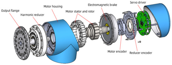
Figure 1.
Structure of robot joint module.
The precision of the robot joint module directly affects the performance and application range of a robot. It can improve the precision and stability of robot movement, and it can make the operation of a robot more stable, accurate, and reliable. Many scholars have carried out research on the precision improvement of robot joint modules. In [8], a method for improving robot joint accuracy based on a mixed motion model and deep learning algorithm was proposed. The model combines static measurement data with dynamic kinematic relationships, and it uses deep neural networks to learn motion features and to achieve high-precision and effective joint reconstruction of the robot, thereby improving the positioning accuracy and control performance. In [9,10], the method of improving the precision of robot joints based on the Kalman filter and parameter adaptation was introduced. Compared with the traditional calibration method, this method has better robustness and stability, can update the robot model parameters in real time, and shorten the calibration time. In [11], an online robot joint precision improvement method based on the weighted recursive least square method and load effect was proposed, which is used to achieve motion control and high-precision state estimation when robots perform complex tasks. The algorithm can effectively optimize robot model parameters and perform real-time compensation in combination with sensors. It makes the robot control achieve more accurate positioning and become more stable, and at the same time it protects the robot drive mechanism.
Robot harmonic reducers generally have involute and triangular tooth profiles [12]. The harmonic reducer studied in this article is the Y series high-precision reducer, which adopts a new structure and tooth design, replacing traditional second harmonic technology. This is a new type of third harmonic tooth. This design creates three contact points between the flexible wheel and the rigid wheel, thereby increasing the number of teeth that can mesh with the gear simultaneously, significantly improving torsional stiffness and transmission accuracy.
In the precision control of harmonic reducers, it is essential to address the issue of gear misalignment, as this can lead to catastrophic consequences for the harmonic reducer, resulting in the failure of both the flexible and rigid wheels [13,14]. There are many reasons for this problem, which may be the material problem of the harmonic reducer, the assembly problem, or the control problem. In fact, vibration will also lead to the shortening of the life of the harmonic reducer when the reducer works in the vibration link for a long time, resulting in excessive wear, which may lead to gear dislocation [15,16].
The purpose of this article is to improve the precision of the harmonic reducer. The harmonic reducer and permanent magnet synchronous motor are first researched as a whole object. The mathematical model of the joint module is then established with the harmonic reducer, and its working principle is studied. The vibration and torque disturbance of the joint module are analyzed to improve the control accuracy of the robot joint module. The ADRC algorithm, combined with the characteristics of the PMSM, harmonic reducer and photoelectric encoder, improves the precision limit of the harmonic reducer, and effectively improves the rigidity and control accuracy of the joint module.
2.2. Mathematical Model of Permanent Magnet Synchronous Motor
The PMSM satisfies the following equation [17]
where and are the d-axis and q-axis inductances of the PMSM, respectively, is the stator resistance, is the stator leakage inductance, and are, respectively, the d-axis and q-axis current of the PMSM, and are, respectively, the d-axis and q-axis voltage of the PMSM, is the angular velocity of the motor, is the electrical angular velocity of the motor, and is the angle of the motor.
2.3. Precision Error Model of Harmonic Reducer
The precision error model of harmonic reducer can be expressed as [18]
where is the transmission ratio of the harmonic reducer, is the output angle of the joint module, and are the precision errors caused by gear meshing deformation and torque output elastic deformation, respectively, and is the precision error caused by other disturbances of the harmonic reducer. These disturbances are superimposed together, resulting in the decline of the control accuracy of the joint module. The larger the value of the latter three terms, the worse the control accuracy [19,20,21].
2.4. Mathematical Analysis of Robot Joint Model
The robot joint torque output equation can be described as
where is the torque of the robot joint module, is the torque output efficiency of the harmonic reducer, J is the moment of inertia, is the number of pole pairs of the motor, is the magnetic flux linkage of the motor rotor, is the friction coefficient, is the angular velocity of the robot joint module, is the external load torque, and is the disturbance term, which includes gear meshing deformation of harmonic reducer, output elastic deformation, and other uncontrollable factors.
This disturbance term can be described in terms of an external torque disturbance term during motion, which can be regarded as the extra torque term added to the joint mathematical model, and the final observed value is the precision error value of the joint module output [22]. The disturbance factors of the robot joint module mainly include the gear meshing deformation and output elastic deformation of the harmonic reducer itself and the vibration of the load, which affect the precision, stability, and life of the robot joint module. These disturbances are briefly described below [23,24].
2.4.1. Meshing Deformation of Gear
The meshing of the gear in the harmonic reducer will cause the stress concentration and the deformation of the wheel, resulting in a change in the tooth clearance, which will have a negative effect on the transmission accuracy. The existence of machining errors and assembly tolerances of parts will further amplify the meshing deformation of gears. At the same time, gear, material, and tangential loads also affect the meshing deformation [25].
2.4.2. Harmonic Reducer Output Elastic Deformation
Because the output shaft system is subjected to torque strain, the position of the tooth surface meshing point is offset, and the output precision is reduced further. The larger the external load, the larger the deformation error. Output elastic deformation is one of the key factors affecting the accuracy of the robot. At the same time, the unstable material machining precision and the harmonic reducer overload can also increase the output elastic deformation module of robot joint motion precision [26].
2.4.3. Vibration of Robot Joint Module
The vibration of joint modules is a common problem in robot movement. Especially when the load changes, it will bring great impact and vibration. At the same time, the internal structural design factors of the joint module or the parts manufacturing tolerances exist, which will also bring the meshing errors of bearings, gears, or other parts, thereby increasing the risk of vibration [27].
The above three disturbance terms are the main reasons for a decrease in the control accuracy of the robot joint module as well as a reduction in the motion accuracy and stability of the robot joint.
2.5. Harmonic Retarder Disturbance Model
The formula of harmonic reducer torque disturbance is described as follows [28]
where is the gear meshing deformation causing the disturbance, is the elastic deformation coefficient of the output shaft of the harmonic reducer, is the elastic deformation of the output shaft, is the vibration coefficient of the joint module, and is the angle disturbance caused by the vibration of the joint module.
Combined with the model characteristics of harmonic reducer, the gear meshing deformation torque in Equation (4) can be calculated by the following equation
where is the distortion factor, is the change in tangential force, is the elastic modulus of the material, is the contact stress concentration coefficient of the tooth surface, is the bending moment of the tooth tip under the action of load, and is the influence coefficient of radial axial deformation.
The elastic deformation of the output axis can be calculated using the following formula [29].
where is the flexural stiffness coefficient of the output shaft, is the tensile and compressive force coefficient of the external load, is the length of the output shaft, and is the length of the bearing. For harmonic reducers, the two ends of the output shaft bearing are, respectively, assembled on support points, and its deformation is zero. Therefore, the boundary conditions of this equation are: when and . If the uneven bearing force of the shaft is considered, the deformation of each point of the bearing may be inconsistent. Therefore, a second-order partial differential Equation (6) is used to describe this deformation.
The relationships between these parameters are complex and difficult to accurately calculate or measure. In fact, these parameters are not invariable, and they have specific relationships with the individual differences in the component tolerance, assembly error and damping of the joint module [30]. Due to the randomness and uncertainty of the disturbance of the robot joint module, the traditional mathematical model cannot fully reflect the actual torque disturbance. In nature, ideal models are obtained according to various assumptions, but the control of robot joint modules is always subject to a variety of external and internal interference. In this article, an improved active disturbance rejection control (ADRC) algorithm is used to identify the external torque disturbance, to improve the control precision of the joint module.
Compared with the previous research methods, the ADRC algorithm has good robustness in control performance for the model uncertainty, parameter change uncertainty, and external interference uncertainty of the robot joint module. A high-order internal model is used to estimate the states of the system and interference signals and implement the effective compensation of the disturbance.
3. ADRC of Robot Joint Module
The improved ADRC is used to improve the disturbance rejection ability of torque. The extended state observer (ESO) is designed to observe the disturbance, and the linear state error feedback (LSEF) is designed to control the torque error to improve the dynamic response accuracy. The function of TD (Tracking Differentiator) is to quickly track the input signal. The control algorithm block diagram is shown in Figure 2 [31,32].
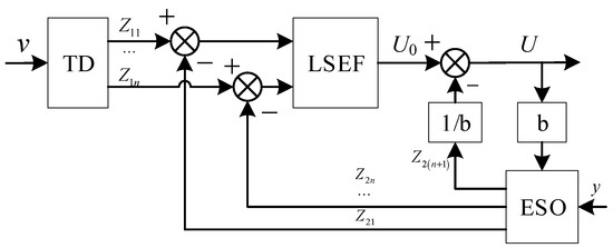
Figure 2.
Disturbance rejection control model.
3.1. Design of Extended State Observer (ESO)
After separating the operating state of the robot joint module from the disturbance term, a system model without disturbance can be obtained.
In the previous analysis, the expression for the external torque disturbance is . All subsequent disturbances are represented by an additional torque term , which is introduced to offset the influence of three disturbances.
The state variable estimated by the disturbance term is defined as
The aim of ADRC is to minimize the value of and make it close to zero, to improve the control accuracy of the robot joint module. In the robot joint module, the high-speed side encoder installed on the motor and the low-speed side encoder installed on the harmonic reducer are used to accurately obtain the data of and .
In order to use ADRC to correct disturbances, an ESO is designed to estimate it, which can be described as
where , , and are the control parameters, and Uq is the q-axis voltage value of the motor. Appendix A verifies the stability of Equation (10). In this system, the model is coupled with the physical model of the joint module, and then the error of the joint angle is assigned to the state vector of the ESO. Then, one can have
where , are the state quantities of the extended second-order observer. The output of this observer can be regarded as an optimal estimate of the disturbance term of the robot joint module, so can be used to estimate the actual disturbance term, i.e., , sgn(e1) represents the saturation function, which is used here to restrict the value range of a single variable to be in a defined interval. The function is defined as follows
where emax and emin are the maximum and minimum values allowed by the saturation function, respectively. For the symbolic function used by the second-order extended state observer in this article, emax = 1 and emin = −1 are usually selected, i.e., e1 is limited to the interval [−1, 1]. The restricted value is used as the input value to calculate the variable , thus ensuring that the output estimation of the observer is not too large or too small.
The output of the ESO is the torque estimation , and the q-axis current estimation . Thus, a complete model of the extended state observer is constructed as follows
where and are the state variables of the extended second-order observer, is the estimated value of the q-axis current, and is the estimated value of the torque disturbance. This torque disturbance value is a quadratic derivative of , and in physical terms, it is an acceleration term, which is the fluctuation of force. The estimator variable is used for sampling current closed-loop control in current loop control, and is used to compensate for external torque interference in current closed-loop control. is the error value of the joint angle accuracy, which can be calculated according to the data of the encoder installed at the end of the motor and the encoder at the end of the joint module. represents the given value of the q-axis voltage of the motor, which is the voltage output command calculated by the current loop controller. , , , are the design parameters of the ESO, which control the convergence speed and observation accuracy of the output state variables [33,34,35].
These physical variables and parameters together form the model of the ESO. In practical application, the model performance and response speed can be optimized by adjusting each parameter to achieve a better control effect. At the same time, the model can compensate the disturbance in the joint module and enhance the stability and robustness of the whole system.
3.2. LSEF Controller Design
After the ADRC algorithm is introduced to obtain the estimated q-axis current, the LSEF controller is described by Equation (14)
where is the current reference value of the q-axis, and and are the proportional and integral gains of the current loop controller, respectively.
3.3. Active Disturbance Rejection Compensation Control Strategy
In order to improve the control precision of the robot joint module, a torque compensation item is designed in the current loop controller to offset the torque disturbance. The specific form is as follows:
where b is the control parameter of the ADRC controller, the value of which determines the strength of the torque active disturbance rejection term. If the value of this parameter is too small, it will lead to the oscillation of the output signal . In theory, the output values of PI controllers need to be limited to avoid saturation of the controller output. After adding the active disturbance rejection algorithm, further limitations must also be imposed on this output. The power supply voltage of the joint module in this article is 48 V, so the output limits of and signals should also be controlled within 48 V to avoid loss of control in specific situations. In this experiment, the following relationship is verified: when the and signals are saturated, the current vector angle of the PMSM cannot always maintain a 90-degree relationship with the rotor magnetic field. At this time, the PMSM will continuously increase the current in order to maintain torque, ultimately leading to the collapse of the entire active disturbance rejection algorithm.
Through the above formula, after introducing the second-order ESO and estimating the torque disturbance value , the uncertain torque disturbance of the robot joint module can be accurately compensated [36,37].
As a result, the block diagram of the ADRC algorithm for the current loop of the robot joint can be obtained, as shown in Figure 3.
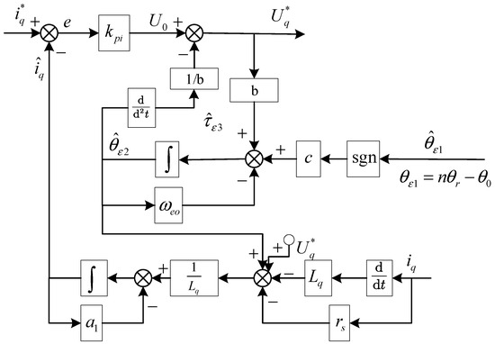
Figure 3.
Current loop active disturbance rejection controller.
In Figure 3, the selection of the active disturbance rejection coefficient, like the tuning of PI parameters, is an experimental process. First, disable the active disturbance rejection control function, adjust the coefficients of the ACR and ASR controllers, and then continuously correct these coefficients based on the waveform of observed in the experiment. From an engineering perspective, it does not have a very strict coefficient reference value. The choice of b has a significant impact on the control effect. If b is less than 0.8, the experimental waveform of is prone to oscillation. For the selection of other coefficients, just like PI parameters, they can be adjusted within a certain range, and their impact on experimental results is within an acceptable range. In this experiment, b = 1.8 is chosen, and other active disturbance rejection coefficients are adjusted appropriately within the range of 0.5~1.5. In fact, b can be understood as a total coefficient, which reflects the strength of the estimated disturbance entering the controller. Control parameters are listed in Table 1.

Table 1.
The list of the parameters.
4. Comparison and Analysis of Experimental Results
4.1. Experimental Method for Performance Test of Robot Joint Module
In traditional robot control, ASR (automatic speed regulator) and ACR (automatic current regulator) generally use PI control. The expression for ASR is:
where and are the proportional and integral coefficients of ASR, is the speed given as the command for the permanent magnet synchronous motor, and is the speed feedback command for the permanent magnet synchronous motor.
The expression of ASR is as follows:
By comparing Equation (15), it can be found that a torque disturbance signal was added to torque current control, which is also the core issue studied in this article. By estimating the disturbance signal through active disturbance rejection control and superimposing it on the output of the current loop controller, the influence of torque disturbance is reduced, thereby improving the control accuracy of the robot joint module.
In order to verify the performance of the ADRC algorithm, the control strategy for comparison testing is first introduced:
4.1.1. PMSM Output Bearing Position Closed-Loop Control Waveform
As shown in Figure 4, the control scheme collects the encoder data θ0 of the PMSM and adopts a vector control strategy to realize three closed-loop controls of position, speed, and current.
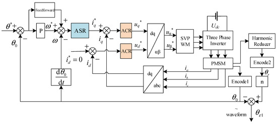
Figure 4.
Position closed-loop control.
Although this control strategy is robust and the algorithm is reliable, it only controls the position of the motor output bearing without considering the influence of external disturbance and the gear meshing error of the harmonic reducer, resulting in poor output accuracy of the joint module. In Figure 4, ASR is an automatic speed regulator, which is a speed loop controller. ACR stands for automatic current regulator, which is a current loop controller.
4.1.2. Harmonic Reducer Output Bearing Position Closed-Loop Control
In response to the shortcomings of the first scheme as shown in Figure 4, some studies read the encoder value of the harmonic reducer end as the position input for vector control, as shown in Figure 5. The position value θr of the harmonic reducer encoder is read, multiplied by the drive ratio n of the robot joint module, and used as the position feedback signal of the PMSM, to realize the closed-loop control of the system. The control strategy improves the control precision and is applied in some situations with a low response requirement and lightweight load. However, if the effect of the harmonic reducer transmission error is considered, the actual position of motor θ0 cannot be calculated by the actual position of joint module θr. When the robot works at high speed, heavy load, and strong disturbance, it easily results in the oscillation of the position loop algorithm.
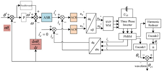
Figure 5.
The encoder value of the harmonic reducer end as the position input for vector control.
4.1.3. Current-Loop ADRC
From the analysis of the oscillation mechanism of the control algorithm, only the closed-loop control for the position value θr at the end of the module is equivalent to ignoring the torque disturbance term, which is related to the load, tolerance, tooth shape, material, and vibration of the harmonic reducer. The larger the disturbance term is, the more likely it is to cause position loop oscillation and lead to poor precision of the joint module, so the controller must consider the influence of this torque disturbance term on the robustness of the system. This is the reason why the current loop ADRC algorithm is used in this article. The position of θr and θ0 is read by two encoders, and the torque interference value is obtained in combination with the ESO model to offset the influence on the control performance, as shown in Figure 6.
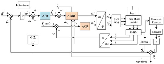
Figure 6.
Combination with the ESO model.
4.2. Experimental Platform
Table 2 lists the parameters of the experimental setup.
Table 2.
The PMSM parameters of the experimental joint module.
Harmonic reducer parameters are as follows: deceleration ratio: 101:1, rated torque: 133 N.m, maximum torque: 217 N.m, single direction positioning accuracy: 30 arcsec, and repeated positioning accuracy: 7 arcsec. The servo driver rated current is 15 A, rated voltage is 48 V. Since the 48 V bus voltage of the robot joint module will increase under the energy feedback braking state, the automatic voltage adjustment device is designed to be connected to the 48 V power supply in parallel, and the voltage is stabilized at 48 V, through the discharge resistance, as shown in Figure 7. The length of the swing arm connected to the joint module is 300 mm, and the end can be installed with different weights for comparison experiments.
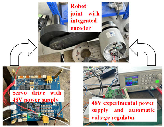
Figure 7.
Experimental platform.
As mentioned above, the control accuracy error is defined as θe1 = nθr − θ0, which describes the actual position value of the motor output shaft of the joint module. After the ADRC algorithm is used to compensate the meshing deformation, output elastic deformation, vibration, and other disturbances of the harmonic reducer, θe1 should be infinitely close to zero, i.e., the input angle θ0 is completely synchronized with the output angle θr, which is also the significance of improving the robot control accuracy. Therefore, it is reasonable to take the value of θe1 as the basis for evaluating the effect of the ADRC algorithm.
The meaning of the vertical axis of all experimental graphics is the angle error value of the two encoders of the robot joint module, which is measured in arc-seconds and is a unit of radians. It is also a universal accuracy evaluation unit for harmonic reducers. In industrial robot applications, the positioning accuracy of harmonic reducers is about 50 arc-seconds. One degree equals 3600 arc-seconds. In the experimental figure, all units are in arc-seconds.
4.3. Experimental Results and Analysis
The fundamental reason for the waveform of in all figures is caused by the elastic deformation of the gear mesh in the harmonic reducer. Each time the gears mesh, an approximate triangular wave of accuracy change is generated. Its period depends on how many gears are engaged in the entire circle of the harmonic reducer. If the transmission ratio of the harmonic reducer changes, the period of will also change accordingly. Due to disturbances in the robot joint module, the amplitude of will increase and the accuracy will deteriorate. The purpose of this study is to reduce disturbances and minimize changes in amplitude.
In the experimental waveform, the vertical axis describes the angle error value. The active disturbance rejection control algorithm studied in this article is aimed at reducing this error value to improve the overall accuracy of robot operation. Observing the data on the vertical axis, it can be observed that the smaller the angle error value, the higher the control accuracy, and the higher the precision of the robot. In the following experiment, the comparative data of angle error values under different control strategies, speeds, and loads are provided.
4.3.1. No-Load Experiment
Some experiments are carried out to verify the theoretical analysis as shown in Figure 8. Figure 8a shows the closed-loop control of the motor output bearing position. The speed of the PMSM is 200 rpm, and the control strategy is a vector control algorithm. The feedback signal of the position closed-loop control is the position value of the PMSM, while the position value at the end of the joint module is not involved in vector control and is only used to calculate the value to obtain the experimental waveform. The control algorithm is used in the existing robot joint module control, and the encoder value at the end of the harmonic reducer is used to find the zero position when the robot is just powered on. In the case of a no-load joint module, the elastic deformation and load vibration caused by external torque can be ignored. Figure 8b is the local magnification of Figure 8a, which shows the peak–peak value under no-load conditions. At this time, it can be seen that the gear meshing deformation error fluctuates from +10 arcseconds to −40 arcseconds.
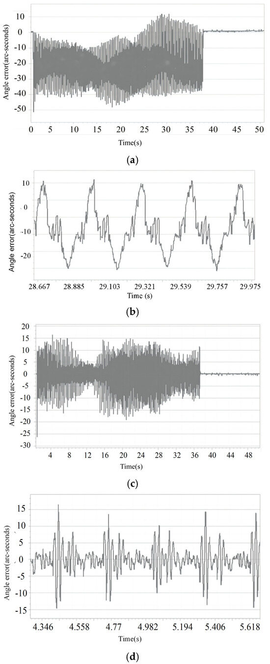
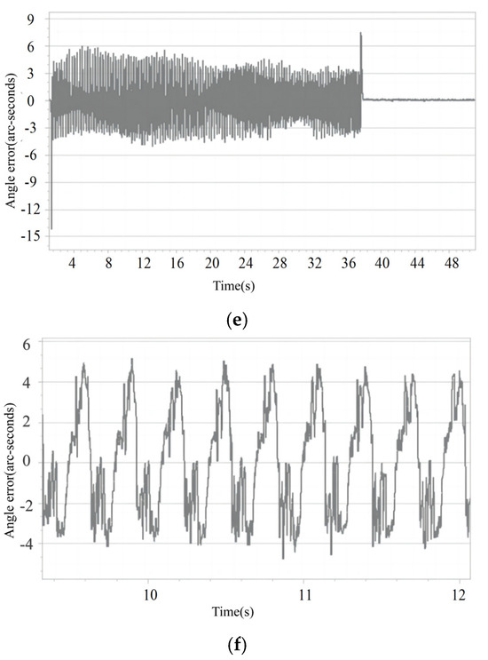
Figure 8.
No load experimental results at speed 200 rpm. (a) PMSM output bearing position closed-loop control waveform1. (b) PMSM output bearing position closed-loop control waveform2. (c) Harmonic reducer output bearing position closed-loop control waveform1. (d) Harmonic reducer output bearing position closed-loop control waveform2. (e) Current loop ADRC waveform1. (f) Current loop ADRC waveform2.
Figure 8c adopts the closed-loop control of the bearing position of the output harmonic reducer, i.e., participates in the vector control operation, while it is only used to calculate the control error. This strategy has good control precision in no-load. Figure 8d is a local enlargement of Figure 8c. It can be seen from Figure 8c that the control accuracy is significantly improved, compared with the strategy of position ring acting on PMSM bearings. The dynamic gear meshing deformation error of the joint module is plus or minus 15 arcseconds. Figure 8e shows the waveform of current loop ADRC, and Figure 8f shows the magnified local waveform. It can be seen from the waveform diagram that the gear meshing error was significantly improved, and the high precision of plus or minus 6 arcseconds was maintained at the speed of 200 rpm, thus breaking the accuracy limit of the reducer itself.
4.3.2. 5 kg Load Experiment
Figure 9a shows the precision error waveform of the PMSM output bearing position closed-loop control under the condition of low speed and a 5 kg load. In this case, the elastic deformation of the joint module is the main disturbance. The load position at the starting point is in the free vertical state, and the joint module is under the minimum force, so the elastic deformation is the minimum. When the joint module rotates to the left and right horizontal position, the force is the largest, and the elastic deformation of gear engagement is the largest. The accuracy is also worse, reaching 70 arcseconds. Figure 9b shows the closed-loop control waveform of the bearing position output of the harmonic reducer under the condition of low speed and a 5 kg load. Compared with the PMSM output bearing position closed-loop control waveform, the control accuracy is obviously improved, and the error fluctuates in the range of plus or minus 20 arcseconds. When the robot joint module starts and brakes, the accuracy error is −70 arcseconds and 100 arcseconds, respectively.
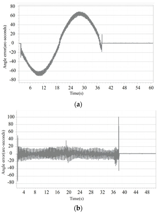
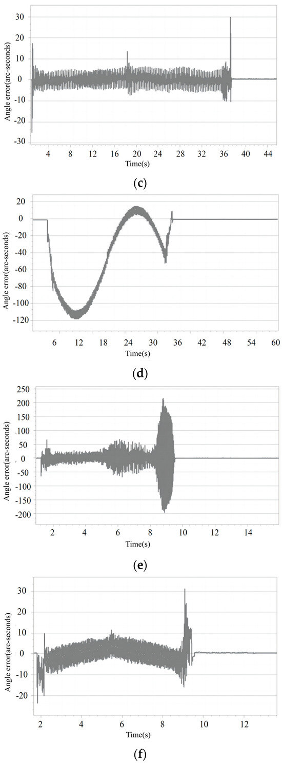
Figure 9.
Experimental results under the condition of motor speed 1000 rpm and motor load 5 kg. (a) PMSM output bearing position closed-loop control waveform. (b) Harmonic reducer output bearing position closed-loop control waveform. (c) Current-loop ADRC waveform. (d) PMSM output bearing position closed-loop control waveform. (e) Harmonic reducer output bearing position closed-loop control waveform. (f) Current-loop ADRC waveform.
Figure 9c shows the current-loop ADRC waveform under the condition of low speed and a 5 kg load. Compared with the closed-loop control strategy of an output bearing position of the harmonic reducer, the control accuracy is further improved. In the uniform motion of the motor at 200 rpm, although the error at the 180-degree position is larger, the remaining error fluctuation is controlled in the range of plus or minus 8 arcseconds, and the error of starting and stopping is also significantly reduced, controlled in the range of plus or minus 30 arcseconds. Figure 9d shows the precision error waveform of the PMSM output bearing position closed-loop control under the condition of high speed and a 5 kg load. The accuracy error range under this condition is very large, with fluctuations ranging from −190 arcseconds to +18 arcseconds.
Figure 9e shows the precision error waveform of the harmonic reducer output bearing position closed-loop control under the condition of high speed and a 5 kg load. The control error produces oscillations and even worsens when the motor stops, indicating that this control strategy will seriously reduce the accuracy and life of the robot under this working condition. In this joint module control strategy, the position of the motor is obtained by reading the joint module position θr and multiplying the drive ratio n of the harmonic reducer. Because of the elastic deformation of the harmonic reducer, the position data contain the disturbance error term. If the disturbance signal is not processed, the robustness of the control system will deteriorate. Figure 9f shows the precision error waveform of the ADRC algorithm under high speed and load conditions. The experimental waveform shows that the error of output precision can be reduced effectively when the torque disturbance is estimated and the ADRC current loop is added. When the PMSM moves at a constant speed at 1000 rpm, the error range is effectively controlled within the range of plus or minus 10 arcseconds. In the start and stop stages, the error fluctuation is convergent, and the accuracy error range is still controlled at plus or minus 30 arcseconds.
From the waveform in Figure 9e, it can be estimated that undergoes drastic changes during the stopping stage, and the corresponding also causes drastic changes. In fact, these changes are caused by the inability of ESO’s output value to converge. In order to ensure the response speed of the robot, the corresponding ACR controller cannot be set too small, otherwise the robot positioning time will become longer. There is always torque disturbance during the operation of the robot, which will be amplified when the robot is under heavy load. The increase in disturbance is also an inevitable result of the elastic deformation of harmonic reducers under heavy loads. Comparing the waveform in Figure 9f, it can be observed that increasing the output value of by dividing the estimated disturbance amount by the coefficient b and feeding it into the active disturbance rejection controller can effectively suppress the disturbance.
4.3.3. Sudden Load Disturbance Experiment
When the PMSM moves at a constant speed of 200 rpm, a torque disturbance of a 2 kg load is added to the end of the swinging arm of the robot joint, and the variation waveform of the joint accuracy error is obtained, as shown in Figure 10a–c. The accuracy error of PMSM output bearing position closed-loop control and harmonic reducer output bearing position closed-loop control are more than 200 arcseconds. However, the ADRC algorithm has an obvious suppression effect on the sudden load disturbance, and the accuracy error can be controlled between plus or minus 50 arcseconds.
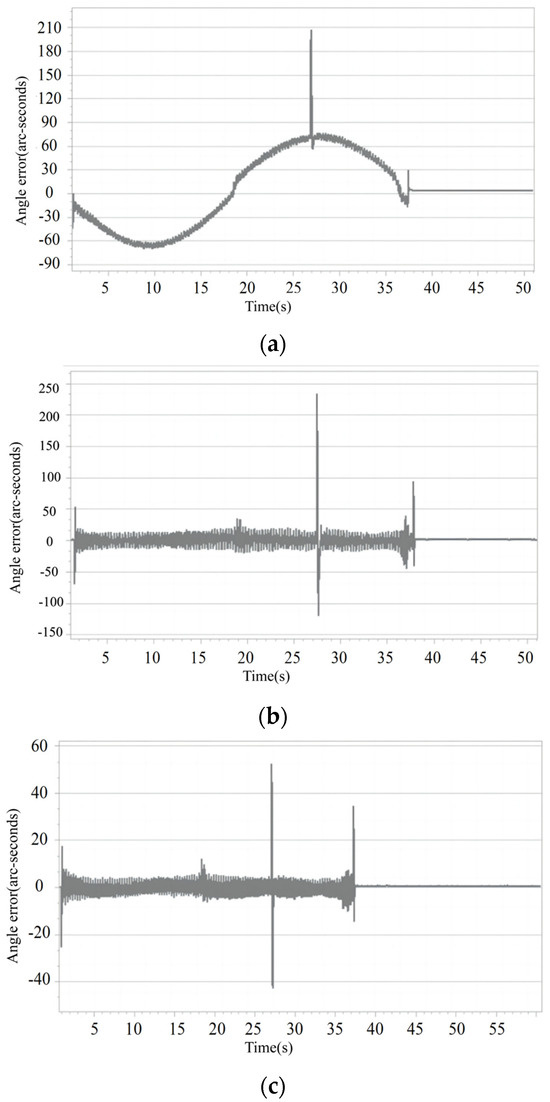
Figure 10.
Sudden load disturbance experiment. (a) PMSM output bearing position closed-loop control sudden load waveform. (b) Sudden load waveform under closed-loop control of PMSM output bearing position. (c) Sudden load waveform under ADRC.
5. Conclusions
ADRC is designed based on modern control theory, with the core of actively sensing and compensating for system disturbances and states to achieve high-performance control. This article estimates and compensates online for torque disturbances and the gear deformation of reducers that affect control accuracy by collecting encoder position information from robot joint modules. It can maintain a good control performance even in the presence of multiple disturbances. Comparing the results of different experimental conditions of three control strategies, the traditional ACR controller has a simple structure, is easy to implement, and can be widely used in situations where accuracy and dynamic characteristics are not required. However, when faced with complex dynamic characteristics and a large amount of uncertain disturbances, ADRC technology performs better due to its strong disturbance rejection ability and robustness. The experimental results show that (1) adding an ADRC algorithm effectively suppresses internal and external disturbances of robot joints and improves the robustness and disturbance rejection ability of the system. (2) Due to its unique structural design, ADRC has a faster response speed and smaller overshoot in robot joint accuracy control. (3) ADRC does not require an accurate system model; it only requires the position information of the two encoders of the robot joints needs to be extracted, and combined with PMSM vector control technology, LESO can be designed, which makes it perform better in the face of uncertain disturbances and complex harmonic reducer dynamic characteristics.
In the robot joint module control, due to the existence of several perturbations of harmonic reducers, the position closed-loop control for angle θ0 or angle θr cannot achieve satisfactory results. By studying the various disturbance factors of the harmonic reducer, this article combines the physical characteristics of the harmonic reducer with the ADRC algorithm to offset the accuracy loss caused by the deformation and vibration of the harmonic reducer gear, to break through the inherent mechanical precision of the harmonic reducer and significantly improve the control accuracy of the robot joint module. The experimental results show that the whole control system has good disturbance rejection performance and good positioning accuracy.
Author Contributions
Conceptualization, G.W. and S.F.; methodology, G.W.; software, G.W.; validation, G.W.; formal analysis, G.W.; investigation, G.W.; resources, G.W.; data curation, G.W.; writing—original draft preparation, G.W.; writing—review and editing, S.F.; visualization, G.W. and S.F.; supervision, S.F.; project administration, S.F.; funding acquisition, S.F. All authors have read and agreed to the published version of the manuscript.
Funding
This research was funded in part by the special fund of Jiangsu Province for the transformation of scientific and technological achievements (No. BA2023048).
Institutional Review Board Statement
Not applicable.
Informed Consent Statement
Not applicable.
Data Availability Statement
The original contributions presented in the study are included in the article, further inquiries can be directed to the corresponding author/s.
Conflicts of Interest
The authors declare no conflicts of interest.
Appendix A
Equation (10) can be rewritten as
To prove its stability, we usually need to consider its equilibrium points and analyze the system’s behavior near these points.
Equilibrium points are points where the system is at rest, which means and Substituting these into Equation (10), one can have:
Solving for , one can have:
This means that can be and , depending on the sign of . To analyze the stability of these equilibrium points, we linearize the system around these points. We consider small perturbations around the equilibrium points and . For the small disturbance , sgn() can be approximated by the sign of , then Equation (10) can be rewritten as
The linearized equation is:
This is a second-order linear homogeneous differential equation with constant coefficients. The characteristic equation is:
Solving for λ, one can have: λ = 0 or λ =
For λ = 0, the solution is , where A is a constant. This indicates that the system is neutrally stable near the equilibrium points.
For λ = , the solution is , where is a constant. Since , this solution decays to zero as t→∞, indicating that the system is asymptotically stable.
References
- Gao, Z. Engineering cybernetics: 60 years in the making. Control Theory Technol. 2014, 12, 97–109. [Google Scholar] [CrossRef]
- Zhang, X.; Huang, J. Active disturbance rejection trajectory tracking control of omnidirectional mobile robot. Mech. Sci. Technol. Aerosp. Eng. 2022, 41, 1869–1876. [Google Scholar]
- Chen, Z.; Ruan, X.; Li, Y. An active disturbance rejection based balance control method for cubic robot. Control Decis. 2019, 34, 1203–1210. [Google Scholar]
- Qiao, G.; Jiang, X.; Nie, X.; Gao, C. Accuracy improvement for industrial robot based on joint position sensitive virtual tool transformation fitting method. In Proceedings of the 2023 6th International Conference on Robotics, Control and Automation Engineering (RCAE), Suzhou, China, 3–5 November 2023; pp. 303–308. [Google Scholar] [CrossRef]
- Peng, T.; Zhang, T.; Sun, Z. Research on robot accuracy compensation method based on modified grey wolf algorithm. In Proceedings of the 2023 8th Asia-Pacific Conference on Intelligent Robot Systems (ACIRS), Xi’an, China, 7–9 July 2023; pp. 1–6. [Google Scholar] [CrossRef]
- Trang, T.; Pham, T.; Yin, Q.; Wang, Q.; Hu, Y.; Li, W. Design harmonic drive for application in robot joint. In Proceedings of the 2022 International Conference on Mechanical and Electronics Engineering (ICMEE), Xi’an, China, 21–23 November 2022; pp. 106–113. [Google Scholar] [CrossRef]
- Park, M.-W. A study on conceptual design of planocentric involute reducer for modular robot. In Proceedings of the 2019 19th International Conference on Control, Automation and Systems (ICCAS), Jeju, Republic of Korea, 15–18 October 2019; pp. 1412–1414. [Google Scholar] [CrossRef]
- Bekey, G.A.; Goldberg, K.Y. (Eds.) Neural Networks in Robotics; Springer Science & Business Media: Berlin/Heidelberg, Germany, 2012; Volume 202. [Google Scholar]
- Sun, F.; Sun, Z.; Woo, P. Neural network-based adaptive controller design of robotic manipulators with an observer. IEEE Trans. Neural Netw. 2001, 12, 54–67. [Google Scholar] [PubMed]
- Hoai-Nhan, N.; Zhou, J.; Kang, H. A calibration method for enhancing robot accuracy through integration of an extended Kalman filter algorithm and an artificial neural network. Neurocomputing 2015, 151, 996–1005. [Google Scholar]
- Bai, M.; Zhang, M.; Zhang, H.; Li, M.; Zhao, J.; Chen, Z. Calibration method based on models and least-squares support vector regression enhancing robot position accuracy. IEEE Access 2021, 9, 136060–136070. [Google Scholar] [CrossRef]
- Litvin, F.L.; Fuentes, A.; Gonzalez-Perez, I.; Carvenali, L.; Kawasaki, K.; Handschuh, R.F. Modified involute helical gears: Computerized design, simulation of meshing and stress analysis. Comput. Methods Appl. Mech. Eng. 2003, 192, 3619–3655. [Google Scholar] [CrossRef]
- Temirkhan, M.; Spitas, C.; Wei, D. A computationally robust solution to the contact problem of two rotating gear surfaces in space. Meccanica 2023, 58, 2455–2466. [Google Scholar] [CrossRef]
- Fuentes-Aznar, A.; Gonzalez-Perez, I. Mathematical definition and computerized modeling of spherical involute and octoidal bevel gears generated by crown gear. Mech. Mach. Theory 2016, 106, 94–114. [Google Scholar] [CrossRef]
- Kolivand, M.; Kahraman, A. An ease-off based method for loaded tooth contact analysis of hypoid gears having local and global surface deviations. ASME J. Mech. Des. 2010, 132, 071004. [Google Scholar] [CrossRef]
- Tariq, H.; Galym, Z.; Amrin, A.; Spitas, C. Assessment of contact forces and stresses, torque ripple and efficiency of a cycloidal gear drive and its involute kinematical equivalent. Mech. Based Des. Struct. Mach. 2022, 52, 1304–1323. [Google Scholar] [CrossRef]
- Li, J. Research on Vector Control System of Permanent Magnet Synchronous Motor Based on DSP. Master’s Thesis, Wuhan University of Technology, Wuhan, China, 2008. [Google Scholar]
- Wang, J. Structural Mechanics Analysis of Harmonic Drive Reducer. Ph.D. Thesis, National University of Defense Technology, Changsha, China, 2011. [Google Scholar]
- Tuttle, T.D. Understanding and Modeling the Behavior of a Harmonic Drive Gear Transmission. Ph.D. Thesis, Massachusetts Institute of Technology, Cambridge, MA, USA, 1992. [Google Scholar]
- Ghorbel, F.H.; Gandhi, P.S.; Alpeter, F. On the kinematic error in harmonic drive gears. J. Mech. Des. 2001, 123, 90–97. [Google Scholar] [CrossRef]
- Zou, C.; Tao, T.; Jiang, G.; Mei, X.; Wu, J. A harmonic drive model considering geometry and internal interaction. Proc. Inst. Mech. Eng. Part C-J. Eng. Mech. Eng. Sci. 2017, 231, 728–743. [Google Scholar] [CrossRef]
- Dhaouadi, R.; Ghorbel, F.H. Modelling and analysis of nonlinear stiffness, hysteresis and friction in harmonic drive gears. Int. J. Model Simul. 2008, 28, 329–336. [Google Scholar] [CrossRef]
- Ma, D.; Yan, S.; Yin, Z.; Yang, Y. Investigation of the friction behavior of harmonic drive gears at low speed operation. In Proceedings of the 2018 IEEE International Conference on Mechatronics and Automation (ICMA), Changchun, China, 5–8 August 2018; IEEE: Piscataway, NJ, USA, 2018; pp. 1382–1388. [Google Scholar]
- Routh, B. Design aspects of harmonic drive gear and performance improvement of its by problems identification: A review. In AIP Conference Proceedings; AIP Publishing: Melville, NY, USA, 2018. [Google Scholar]
- Tuttle, T.D.; Seering, W.P. Kinematic error, compliance, and friction in a harmonic drive gear transmission. In Proceedings of the International Design Engineering Technical Conferences and Computers and Information in Engineering Conference, Albuquerque, NM, USA, 19–22 September 1993; American Society of Mechanical Engineers: New York, NY, USA, 1993. [Google Scholar]
- Yamamoto, M.; Iwasaki, M.; Hirai, H.; Okitsu, Y.; Sasaki, K.; Yajima, T. Modeling and compensation for angular transmission error in harmonic drive gearings. IEEJ Trans. Electr. Electron. Eng. 2009, 4, 158–165. [Google Scholar] [CrossRef]
- Gandhi, P.S.; Ghorbel, F.H. Closed-loop compensation of kinematic error in harmonic drives for precision control applications. IEEE Trans. Control Syst. Technol. 2002, 10, 759–768. [Google Scholar] [CrossRef]
- Iwasaki, M.; Yamamoto, M.; Hirai, H.; Okitsu, Y.; Sasaki, K.; Yajima, T. Modeling and compensation for angular transmission error of harmonic drive gearings in high precision positioning. In Proceedings of the 2009 IEEE/ASME International Conference on Advanced Intelligent Mechatronics, Singapore, 14–17 July 2009; IEEE: Piscataway, NJ, USA, 2009. [Google Scholar]
- Dong, H.; Dong, B.; Zhang, C.; Wang, D. An equivalent mechanism model for kinematic accuracy analysis of harmonic drive. Mech. Mach. Theory 2022, 173, 104825. [Google Scholar] [CrossRef]
- Taghirad, H.D.; Belanger, P.R. Torque ripple and misalignment torque compensation for the built-in torque sensor of harmonic drive systems. IEEE Trans. Instrum. Meas. 1998, 47, 309–315. [Google Scholar] [CrossRef]
- Xie, J.; Wei, W.; Liao, P.; Liu, J. Design of ADRC controller for induction motor based on improved fal function. In Proceedings of the 2022 14th International Conference on Advanced Computational Intelligence (ICACI), Wuhan, China, 15–17 July 2022; IEEE: Piscataway, NJ, USA, 2022. [Google Scholar]
- Liu, B.; Hong, J.; Wang, L. Linear inverted pendulum control based on improved ADRC. Syst. Sci. Control Eng. 2019, 7, 1–12. [Google Scholar] [CrossRef]
- Deng, F.; Guan, Y. PMSM vector control based on improved ADRC. In Proceedings of the 2018 IEEE International Conference of Intelligent Robotic and Control Engineering (IRCE), Lanzhou, China, 24–27 August 2018; IEEE: Piscataway, NJ, USA, 2018. [Google Scholar]
- Su, G. Fuzzy ADRC controller design for PMSM speed regulation system. Adv. Mater. Res. 2011, 201, 2405–2408. [Google Scholar] [CrossRef]
- Su, Y.; Zheng, C.; Duan, B. Automatic disturbances rejection controller for precise motion control of permanent-magnet synchronous motors. IEEE Trans. Ind. Electron. 2005, 52, 814–823. [Google Scholar] [CrossRef]
- Hezzi, A.; Ben Elghali, S.; Bensalem, Y.; Zhou, Z.; Benbouzid, M.; Abdelkrim, M.N. ADRC-based robust and resilient control of a 5-phase PMSM driven electric vehicle. Machines 2020, 8, 17. [Google Scholar] [CrossRef]
- Tian, M.; Wang, B.; Yu, Y.; Dong, Q.; Xu, D. Discrete-time repetitive control-based ADRC for current loop disturbances suppression of PMSM drives. IEEE Trans. Ind. Inform. 2021, 18, 3138–3149. [Google Scholar] [CrossRef]
Disclaimer/Publisher’s Note: The statements, opinions and data contained in all publications are solely those of the individual author(s) and contributor(s) and not of MDPI and/or the editor(s). MDPI and/or the editor(s) disclaim responsibility for any injury to people or property resulting from any ideas, methods, instructions or products referred to in the content. |
© 2024 by the authors. Licensee MDPI, Basel, Switzerland. This article is an open access article distributed under the terms and conditions of the Creative Commons Attribution (CC BY) license (https://creativecommons.org/licenses/by/4.0/).