Article

An Optimization Method for Green Permutation Flow Shop Scheduling Based on Deep Reinforcement Learning and MOEA/D

College of Mechanical Engineering, Xinjiang University, Urumqi 830046, China
*
Author to whom correspondence should be addressed.
Machines 2024, 12(10), 721; https://doi.org/10.3390/machines12100721 (registering DOI)
Submission received: 15 August 2024 / Revised: 26 September 2024 / Accepted: 9 October 2024 / Published: 11 October 2024
(This article belongs to the Section Advanced Manufacturing)

Abstract

:
This paper addresses the green permutation flow shop scheduling problem (GPFSP) with energy consumption consideration, aiming to minimize the maximum completion time and total energy consumption as optimization objectives, and proposes a new method that integrates end-to-end deep reinforcement learning (DRL) with the multi-objective evolutionary algorithm based on decomposition (MOEA/D), termed GDRL-MOEA/D. To improve the quality of solutions, the study first employs DRL to model the PFSP as a sequence-to-sequence model (DRL-PFSP) to obtain relatively better solutions. Subsequently, the solutions generated by the DRL-PFSP model are used as the initial population for the MOEA/D, and the proposed job postponement energy-saving strategy is incorporated to enhance the solution effectiveness of the MOEA/D. Finally, by comparing the GDRL-MOEA/D with the MOEA/D, NSGA-II, the marine predators algorithm (MPA), the sparrow search algorithm (SSA), the artificial hummingbird algorithm (AHA), and the seagull optimization algorithm (SOA) through experimental tests, the results demonstrate that the GDRL-MOEA/D has a significant advantage in terms of solution quality.

1. Introduction

The permutation flow shop scheduling problem (PFSP), as a classical challenge in the domain of combinatorial optimization problems (COPs), has long been a focal point of intense research and enthusiasm within the international academic community. The key to solving this problem lies in designing algorithms that are efficient, fast, and accurate to fulfill the stringent requirements of contemporary manufacturing for both production efficiency and product quality. In the flow line production environment, this scheduling problem is particularly prominent in industries such as automobile assembly, electronic product manufacturing, food processing, steel, textiles, aerospace, and pharmaceutical processing. Therefore, the successful resolution of this problem not only significantly enhances the efficiency of the production process, but also holds promise for opening up new avenues for innovation and development in the entire manufacturing industry.
Currently, the methods for solving the permutation flow shop scheduling problem are mainly divided into two categories: exact algorithms and approximate algorithms. Exact algorithms aim to find the optimal solution by exhaustively enumerating and evaluating all possible scheduling options, such as branch and bound [1], dynamic programming [2], and integer programming [3]. These methods can theoretically guarantee the optimal solution. However, when faced with large-scale practical problems, due to constraints on computational resources and the “combinatorial explosion” phenomenon, exact algorithms often become impractical. Conversely, approximation algorithms aim to quickly find “good enough” solutions rather than theoretically optimal ones. They can provide practical solutions within a reasonable timeframe for addressing large-scale and complex problems, which are further categorized into heuristic and metaheuristic methods. Heuristic methods encompass the Campbell Dudek Smith algorithm (DCS) [4], the Gupta algorithm [5], the Nawaz Enscore Ham algorithm (NEH) [6], and a variety of scheduling rules [7], with NEH widely regarded as the most effective approach for resolving PFSP [8,9,10,11]. Nevertheless, these heuristic algorithms often operate under simplified assumptions or rules, which may limit their ability to deliver optimal or satisfactory solutions in the face of complex scheduling challenges. Metaheuristic methods, which simulate natural processes or leverage specific heuristic rules, guide the search process to yield satisfactory scheduling solutions and have achieved a series of results in solving PFSP. For example, Zheng et al. [12] developed a hybrid bat optimization algorithm that incorporates variable neighborhood structure and two learning strategies to address the PFSP. Chen et al. [13] proposed a hybrid grey wolf optimization method with a cooperative initialization strategy for solving the PFSP with the objective of minimizing the maximum completion time. Tian et al. [14] proposed a novel cuckoo search algorithm for solving the PFSP. Khurshid et al. [15] proposed a hybrid evolutionary algorithm that integrates an improved evolutionary global search strategy and a simulated annealing local search strategy for solving the PFSP. Razali [16] combined the NEH algorithm with the artificial bee colony algorithm (ABC) to solve the PFSP, which enhances the convergence speed of the ABC. Qin et al. [17] aimed to minimize the completion time and proposed a hybrid cooperative coevolutionary search algorithm (HSOS) based on the cooperative coevolutionary search algorithm combined with local search strategies to solve the PFSP. Rui et al. [18] introduced a multi-objective discrete sine optimization method (MDSOA) to address the mixed PFSP, aiming to minimize the makespan and the maximum tardiness. Yan et al. [19] introduced a novel hybrid crow search algorithm (NHCSA) that enhances the quality of the initial population through an improved version of the NEH method. It employs the smallest-position-value rule for encoding discrete scheduling problems and incorporates a local search mechanism, which is designed to solve the PFSP with the objective of minimizing the maximum completion time. It is evident that metaheuristic algorithms have achieved satisfactory results and performance in the application of PFSP, but their iterative search process is often time-consuming, and they do not fully utilize historical information to optimize and adjust the search strategy. Therefore, there is still significant potential for optimization in solving large-scale problems. For existing specific scheduling problems, delving into the essence of the problem and designing optimization strategies accordingly is crucial. Additionally, rationally utilizing historical information to adjust the search patterns of the algorithms is another key approach to achieve efficient solutions.
In recent years, the rapid advancements in artificial intelligence and machine learning technologies have yielded remarkable achievements across various domains, including speech recognition [20], energy management [21], image processing [22], pattern recognition [23], healthcare [24], and traffic management [25], opening new avenues for solving complex COPs. Consequently, the academic community has started to investigate the application of machine learning techniques to COPs, quickly becoming a research focal point and yielding abundant results. For example, Vinyals et al. [26] introduced Pointer Networks (PN) as an innovative strategy for tackling sequence-to-sequence modeling issues. Ling et al. [27] developed a fully convolutional neural network that learns the optimal solution from the feasible domain to solve the traveling salesman problem (TSP). However, the neural networks employed in the aforementioned approaches are all trained and refined on labeled data, where the quality of the labels directly impacts their performance, a category that is known as supervised learning. Additionally, collecting high-quality data for combinatorial optimization problems (COPs) is a time-consuming and expensive process that requires substantial computational resources and expertise to solve complex problems and generate accurate labels. Therefore, exploring neural network models that can effectively solve COPs is an important topic that urgently needs to be addressed in current research.
Reinforcement learning (RL), unlike supervised learning methods, is a machine learning approach based on a reward mechanism, where an agent learns the optimal strategy through interactions with the environment. In RL, the agent does not rely on a pre-labeled dataset but instead explores the environment, performs actions, and receives feedback. Through this process, the agent gradually adjusts its behavioral strategies, thereby finding the best solution in a dynamically changing environment. This offers an efficient and adaptable method for solving COPs, yielding substantial advancements and real-world applications in challenging domains, including the TSP, vehicle routing problem (VRP), and workshop scheduling problem. To solve the TSP, Zhang et al. [28] proposed a manager–worker deep reinforcement learning (DRL) network architecture based on a graph isomorphism network (GIN) for solving the multiple-vehicle TSP with time windows and rejections. Luo et al. [29] proposed a DRL approach that incorporates a graph convolutional encoder and a multi-head attention mechanism decoder, aimed at addressing the limitations of existing machine learning methods in solving the TSP, which typically does not fully utilize hierarchical features and can only generate single permutations. Bogyrbayeva et al. [30] proposed a hybrid model that combines an attention-based encoder with a long short-term memory (LSTM) network decoder to address the inefficiency of attention-based encoder and decoder models in solving the TSP involving drones. Gao et al. [31] developed a multi-agent RL approach based on gated transformer feature representation to improve the solution quality of multiple TSPs. To solve the VRP, Wang et al. [32] proposed a method that combines generative adversarial networks with DRL to solve the VRP. Pan et al. [33] presented a method that can monitor and adapt to changes in customer demand in real time, addressing the issue of uncertain customer needs in VRP. Wang et al. [34] proposed a two-stage multi-agent RL method based on Monte Carlo tree search, aiming for efficient and accurate solutions to the VRP. Xu et al. [35] developed an RL model with a multi-attention aggregation module that dynamically perceives and encodes context information, addressing the issue of existing RL methods not fully considering the dynamic network structure between nodes when solving VRPs. Zhao et al. [36] proposed a DRL approach for large-scale VRPs that consists of an attention-based actor, an adaptive critic, and a routing simulator. To solve workshop scheduling problems, Si et al. [37] designed an environment state based on a multi-agent architecture using DRL to solve the job shop scheduling problem (JSSP). Chen et al. [38] proposed a deep reinforcement learning method that integrates attention mechanisms and disjunctive graph embedding to solve the JSSP. Shao et al. [39] redesigned the state space, action space, and reward function of RL to solve the flexible job shop scheduling problem (FJSSP) with the objective of minimizing completion time. Han et al. [40] proposed an end-to-end DRL method based on an encoder and a decoder to solve the FJSSP. Yuan et al. [41] constructed a DRL framework based on a multilayer perceptron for extracting environmental state information to solve the FJSSP, which enhances the computational efficiency and decision-making capabilities of the algorithm. Wan et al. [42] developed a DRL approach based on the actor–critic framework to address the FJSSP with the objective of minimizing the makespan. Peng et al. [43] presented a multi-agent RL method with double Q-value mixing for addressing the extended FJSSP characterized by technological and path flexibility, a variable transportation time, and an uncertain environment. Wu et al. [44] proposed a DRL approach for the dynamic job shop scheduling problem (DJSSP) with an uncertain job processing time that incorporates proximal policy optimization (PPO) enhanced by hybrid prioritized experience replay. Liu et al. [45] introduced a multi-agent DRL framework that can autonomously learn the relationship between production information and scheduling objectives for solving the DJSSP. Gebreyesus et al. [46] presented an end-to-end scheduling model based on DRL for the DJSSP, which utilizes an attention-based Transformer network encoder and a gate mechanism to optimize the quality of solutions. Wu et al. [47] introduced a DRL scheduling model combined with a spatial pyramid pooling network (SPP-Net) to address the DJSSP. The model employs novel state representation and reward function design and is trained using PPO. Experiments in both static and dynamic scheduling scenarios demonstrated that this method outperforms existing DRL methods and paired priority. Su et al. [48] developed a DRL method based on the graph neural network (GNN) for the DJSSP with machine failures and stochastic processing time, which utilizes GNN to extract state features and employs evolutionary strategies (ES) to find the optimal policies. Liu et al. [49] developed a DRL framework that employs GNN to convert disjunctive graph states into node embeddings and is trained using the PPO algorithm for solving the DJSSP with random job arrivals and random machine failures. Zhu et al. [50] proposed a method based on deep reinforcement learning to solve the DJSSP. Tiacci et al. [51] successfully integrated the DRL agent with a discrete event simulation system to tackle a dynamic flexible job shop scheduling problem (DFJSSP) with new job arrivals and machine failures. Zhang et al. [52] proposed a DRL method integrated with a GNN to address the DFJSSP with uncertain machine processing time, training the agents using the PPO algorithm, and demonstrating through experiments that this method outperforms traditional algorithms and scheduling rules in both static and dynamic environments. Chang et al. [53] put forward a hierarchical deep reinforcement learning method composed of a double deep Q-network (DDQN) and a dueling DDQN to solve the multi-objective DFJSSP. Zhou et al. [54] proposed a DRL method that uses a disjunctive graph to represent the state of the environment for solving the PFSP. Pan et al. [55] designed an end-to-end DRL framework to solve the PFSP with the objective of minimizing the completion time. Wang et al. [56] introduced a DRL method based on a long short-term memory (LSTM) network to address the non-PFSP. Table 1 summarizes the common methods for solving PFSP, as well as the application of RL in dealing with various shop scheduling problems.
In summary, RL can learn how to make optimal decisions through interaction with the environment, offering effective solutions for combinatorial optimization problems such as the TSP, VRP, and workshop scheduling problem. However, there are several shortcomings in the existing research on using RL to solve the workshop scheduling problem:
  • Firstly, most researchers have focused their studies primarily on the static JSSP [37,38], static FJSSP [39,43], DJSSP [44,45,46,47,48,49,50], and DFJSSP [51,52,53], with relatively less research on PFSP [54,55,56].
  • Secondly, the optimization goal of most research is to minimize completion time, with little consideration given to other objectives such as energy consumption, machine utilization, and delivery time. However, as an essential aspect of manufacturing, energy consumption has become increasingly significant due to its dual impact on production costs and the environment. Therefore, implementing an effective energy-saving strategy in production scheduling not only helps to reduce production costs and enhance the competitiveness of enterprises, but also reduces carbon emissions. It aligns with the global green environmental trend and promotes the achievement of sustainable development goals.
  • Furthermore, in existing research, the state of the environment for RL algorithms is typically constructed as a set of performance indicators, with each indicator usually mapped to a specific feature. However, the intricate correlations among these performance indicators lead to a complex internal structure of the environmental state, which may contain a large amount of redundant information. This complexity not only increases the difficulty of convergence for neural networks, but may also negatively impact the decision-making process of the agent, reducing the accuracy and efficiency of its decisions.
  • Finally, in existing research, the action space of the agent is often limited to a series of heuristic rules based on experience. While these rules are easy to understand and implement, they may restrict the exploration of the agent, preventing it from fully uncovering and executing more complex and efficient scheduling strategies.
The multi-objective evolutionary algorithm based on decomposition (MOEA/D), as a classic and effective multi-objective optimization method, is favored by many scholars for its intuitive understandability, high robustness, simple parameter setting, and adaptability to a variety of complex problems. These characteristics make the algorithm particularly prominent in solving job shop scheduling problems and have become a commonly adopted approach by scholars in dealing with such challenges. In recent years, MOEA/D has been applied to solve multi-objective permutation flow shop scheduling problems by breaking down complex multi-objective problems into multiple sub-problems for independent optimization and using Chebyshev aggregation functions to guide the convergence process of the population [57,58]. However, it is worth noting that MOEA/D is highly dependent on the initial solutions, and the quality of the initial solutions will directly affect the overall performance of the algorithm. This feature requires special attention to the generation strategy of initial solutions when using MOEA/D to ensure that the algorithm can achieve the best results.
Therefore, in response to the aforementioned issues, this paper proposes an innovative algorithmic framework that integrates DRL with the MOEA/D algorithm (GDR-MOEA/D) to address the green permutation flow shop scheduling problem, aiming to minimize the objectives of maximum completion time and total energy consumption. The main contributions of this paper are as follows:
  • Firstly, for the existing end-to-end deep reinforcement learning network, which is difficult to apply to different scales of the green permutation flow shop scheduling problem (GPFSP) considering energy consumption, we designed a network model based on DRL (DRL-PFSP) to solve PFSP. This network model does not require any high-quality labeled data and can flexibly handle PFSPs of various sizes, directly outputting the corresponding scheduling solutions, which greatly enhances the practicality and usability of the algorithm.
  • Secondly, the DRL-PFSP model is trained using the actor–critic RL method. After the model is trained, it can directly generate scheduling solutions for PFSPs of various sizes in a very short time.
  • Furthermore, in order to significantly enhance the quality of solutions produced by the MOEA/D algorithm, this study innovatively employs solutions generated by the DRL-PFSP model as the initial population for MOEA/D. This approach not only provides MOEA/D with a high-quality starting point, but also accelerates the convergence of the algorithm and improves the performance of the final solutions. Additionally, to further optimize the energy consumption target, a strategy of job postponement for energy saving is proposed. This strategy reduces the machine’s idle time without increasing the completion time, thereby achieving further optimization of energy consumption.
  • Eventually, through comparative analysis of simulation experiments with the unimproved MOEA/D, NSGA-II, MPA, SSA, AHA, and SOA, the GDRL-MOEA/D model algorithm constructed in this study demonstrated superior performance. The experimental results reveal that the solution quality of GDRL-MOEA/D was superior to the other six algorithms in all 24 test cases. In terms of solution speed, GDRL-MOEA/D was not significantly different from the other algorithms, and the difference was within an acceptable range.
The remainder of this paper is organized as follows. The mathematical model of the GPFSP and the objective functions are presented in Section 2. In Section 3, the proposed GDRL-MOEA/D framework is elaborately concluded. Section 4 presents simulation experiments that assess the proposed algorithm against traditional methods, validating its efficiency. Finally, Section 5 offers a comprehensive summary and an outlook on the future of the work.

2. Multi-Objective Optimization Model for the GPFSP

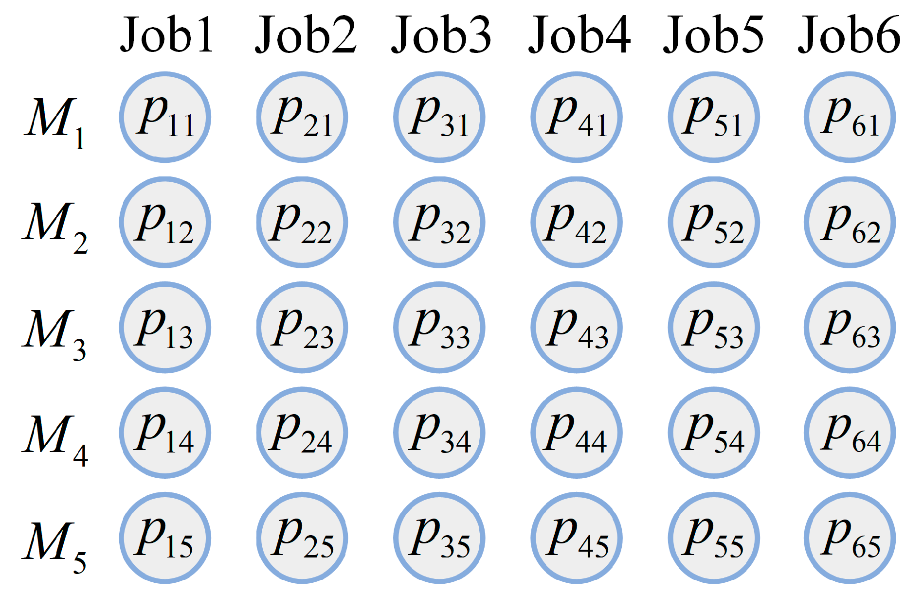
2.1. Problem Description

The GPFSP in this paper can be described as follows: there are n jobs J = J 1 , J 2 , , J n that need to be processed on m machines M = M 1 , M 2 , , M m at the initial moment. Each job follows the same production route through all the machines, starting from machine M 1 , M 2 , M 3 , and so on, until all operations are completed on the last machine M m . The processing time p i j of job i on machine M j is known, and the processing power and idle power of each machine are also determined. The objective of this paper is to determine an optimal sequence π * = π 1 , π 2 , π 3 , , π n for the GPFSP that minimizes the maximum completion time for all jobs and the total energy consumption of all machines. In general, the PFSP is based on the following assumptions:
  • All jobs are mutually independent and can be processed at the initial moment;
  • Only one job can be processed on each machine at any given time;
  • Each job needs to be processed on each machine exactly once;
  • All jobs have the same processing sequence on each machine;
  • The job cannot be interrupted once it starts processing on a machine;
  • The transportation and setup times of jobs between different machines are either disregarded or incorporated into the processing time of the jobs.
Figure 1 exhibits an example of a PFSP scheduling scheme for 6 jobs on 5 machines, with the figure elaborately detailing the processing sequence of each job on every machine. Namely, the sequence of the scheduling plan is π = 3 , 1 , 2 , 5 , 4 , 6 .

2.2. Notations

The notations employed in this article are presented in Table 2.

2.3. Optimization Objectives

The GPFSP model in this paper consists of optimization objectives and constraint equations, aiming to minimize the maximum completion time of jobs and the total energy consumption of machines. The detailed modeling steps of this model are as follows.

2.3.1. Makespan

The first optimization objective is to minimize the maximum completion time of jobs, which can be represented by Equation (1).
min C max = min max F i j = min max S i j + T i j k

2.3.2. Total Energy Consumption

The second optimization objective is to minimize the total energy consumption E , which is the sum of the processing energy consumption and the idle energy consumption of all machines within the maximum completion time C max , as represented by Equation (2).
min E = min i , i = 1 n j = 1 q i k = 1 m a i j k X i j k T i j k + b k ( S i j C i j ) X i j k X i j k X i i
To sum up, the model of GPFSP can be expressed as follows:
min f 1 = min C max
min f 2 = min E
which is subject to:
S i j F i j 1 i , j > 1
k = 1 m X i j k = 1 i , j
S i j 0 i , j
F i j > 0 i , j
F i j = T i j k + S i j i , j
C max C i j i , j
X i j k 0 , 1 i , j , k
X i i 0 , 1 i , i
Equations (3) and (4) individually denote the minimization of the maximum completion time and the total energy consumption for the GPFSP. Equation (5) indicates that a job can only commence the processing of the current operation after the completion of the previous operation. Equation (6) states that each machine can process only one job at any given time. Equations (7) and (8), respectively, indicate that the start time and completion time of a job must not be negative. Equation (9) indicates that, once a job starts processing on a machine, the processing cannot be interrupted. Equation (10) represents the constraint of the makespan. Equations (11) and (12) specify the permissible values for the decision variables.

3. The Solution Framework of the GDRL-MOEA/D

In this section, we propose a framework named GDRL-MOEA/D that combines DRL, MOEA/D, and the energy-saving strategy to address the GPFSP. The specific framework of GDRL-MOEA/D is shown in Figure 2, and the brief process is as follows.
  • First, with the objective of minimizing the maximum completion time, we applied an end-to-end deep reinforcement learning strategy (DRL-PFSP) to model the PFSP problem in Section 3.1 and systematically trained the model using the actor–critic algorithm. Once the DRL-PFSP model is trained, it can efficiently provide high-quality solutions for PFSP instances of varying sizes and complexities.
  • Next, in Section 3.2, these solutions are used as the initial population for MOEA/D to further optimize the scheduling results, forming the DRL-MOEA/D approach. This integrated method improves the efficiency and adaptability of the solving process while maintaining the optimization quality of the solutions.
  • Finally, in order to further reduce energy consumption without increasing the completion time, an innovative energy-saving strategy is proposed in Section 3.3. This strategy optimizes the energy consumption of the scheduling plans generated by DRL-MOEA/D, aiming to achieve more environmentally friendly and efficient workshop scheduling.
The details of each subsection are as follows.

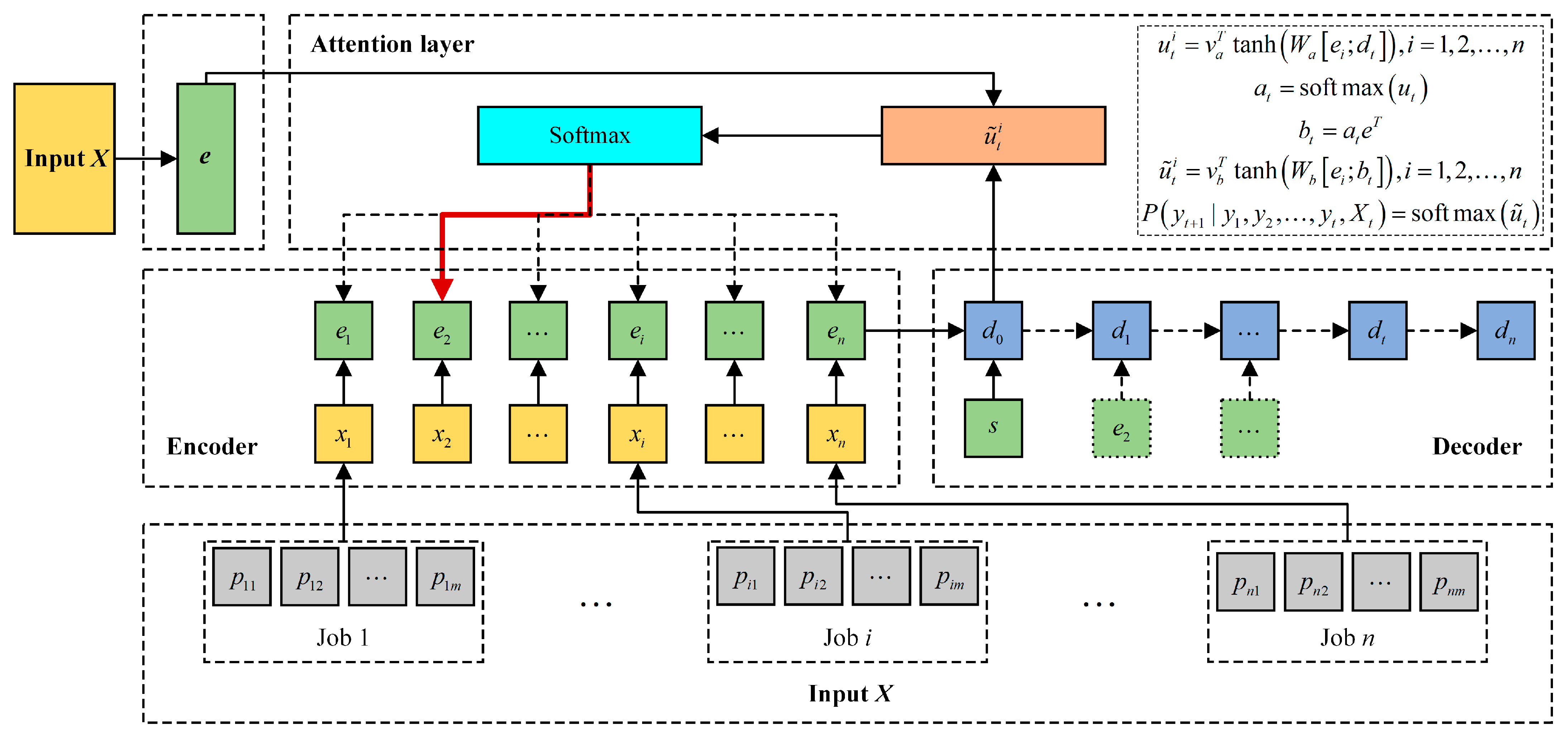
3.1. The Structure of the DRL-PFSP

This section utilizes the PN neural network approach to model the PFSP and employs the actor–critic algorithm for training the model. Figure 3 depicts the comprehensive structure of this approach, which consists of the input layer, encoding layer, decoding layer, and attention layer. In brief, the encoder processes the input sequence (processing times of jobs in this paper) by converting each element into a hidden state vector, forming the encoded representation of the input. Then, at each step, the decoder compares the current decoding state with the hidden states from the encoder through the attention mechanism. The attention mechanism calculates relevance weights for each input position, and these weights are converted into a probability distribution using the softmax function, indicating which element the decoder should prioritize. Based on these weights, the decoder dynamically selects the output elements, gradually generating the complete output sequence. A detailed elucidation of each component will be provided in the subsequent sections.

3.1.1. Input Layer

The input layer is constructed from a sequence of n fixed-dimensional vectors X = x i , i = 1 , 2 , , n , which is employed as the input for the encoding layer. Here, n represents the number of jobs, and each x i is composed of a tuple p i = p i 1 , p i 2 , , p i m . p i j denotes the processing time of job i on machine M j . Using the PFSP instance with six jobs and five machines as a case study, the structure of the encoder’s input is depicted in Figure 4.

3.1.2. Encoding Layer

The function of the encoder is to recognize the input sequence and extract the features of the jobs, subsequently encoding this information into vectors of a fixed dimension. In conventional PN models, recurrent neural networks (RNNs) typically serve as encoders, tasked with the collection and integration of input data and its sequential order. This is especially important in tasks like machine translation, where the sequence of words is vital to the precision of the translation outcome. However, with regard to the job scheduling problem discussed in this paper, the input jobs are all independent entities without any temporal sequence connection between them. Therefore, the encoder in this study utilizes a straightforward one-dimensional (1-D) convolution embedding layer to replace the complex RNN structure, encoding the input data into a high-dimensional vector. This approach not only significantly reduces the model’s complexity, but also effectively decreases the computational cost. And the number of input channels for a 1D convolutional layer corresponds to the dimensionality of the input data. Taking the PFSP with six jobs and five machines in Figure 4 as an example, there are five input channels of the convolutional layer. The encoder ultimately transforms the input data into a vector of dimensions n × d h , where n denotes the quantity of jobs and d h represents the number of neurons in the hidden layer. A key point to note is that all jobs share the parameters of the convolutional neural network. This means that, regardless of the number of jobs, each one utilizes the same set of parameters to encode job information into a high-dimensional vector. Consequently, the encoder demonstrates good robustness in handling varying numbers of jobs.

3.1.3. Decoding Layer

The role of decoder is to accurately decode the high-dimensional vectors outputted by the encoder, which encapsulate the rich knowledge information of the input sequence. Its ultimate objective is to produce an output sequence that closely mirrors the original input sequence in both semantics and structure, ensuring no errors are introduced. Unlike the encoder, the decoder contains an RNN that summarizes the information from the previously selected jobs ρ 1 , ρ 2 , , ρ t to determine the next job ρ t + 1 . The unique advantage of RNN lies in its inherent cyclic structure, which enables it to effectively retain and remember the output information processed previously. This allows it to consider historical context when dealing with sequential data, enhancing the model’s ability to capture temporal dynamics. The decoder network structure employed in this paper is based on gated recurrent unit (GRU), a variant of RNN, which has fewer network parameters compared to the long short-term memory (LSTM) used in the original pointer network. In each decoding step t , the GRU decoder synthesizes the hidden state d t , encapsulating the knowledge from the previous steps ρ 1 , ρ 2 , , ρ t with the input’s encoded representation e 1 , e 2 , , e n , jointly calculating the conditional probability P ρ t + 1 | ρ 1 , ρ 2 , , ρ t , X t for the next action selection. This calculation is performed through an attention mechanism, as shown in Figure 3.

3.1.4. Attention Layer

At each stage of decoding, the attention layer is responsible for receiving the context vectors e output by the encoder and the current decoding vector d t from the decoder. This layer quantifies the association between each job and the potential next job, identifying the job with the highest association as the preferred candidate for the subsequent job. The specific calculation steps are detailed as follows [59]:
u t i = v a T tanh W a e i ; d t , i = 1 , 2 , , n
a t = soft max u t
b t = a t e T
u ˜ t i = v b T tanh W b e i ; b t , i = 1 , 2 , , n
P ρ t + 1 | ρ 1 , ρ 2 , , ρ t , X t = soft max u ˜ t
where “;” denotes the combination of two vectors; v a , v b , W a , and W b all represent the learnable parameters of the model; and a t and b t , respectively, correspond to the “attention” mask for the inputs and the context vector at time step t . The softmax function is utilized to normalize both u t and u ˜ t , resulting in the probability distribution for selecting each job i during step t. As depicted in Figure 3, job 2 exhibits the highest probability value P ρ t + 1 | ρ 1 , ρ 2 , , ρ t , X t , and is therefore selected as the next job to be visited. During the training process, the model does not select the job with the highest probability in a greedy manner, but instead determines the next job by sampling from the probability distribution.

3.1.5. The Training Method for PFSP

This study utilizes a well-regarded actor–critic policy gradient technique to tackle the training challenges of PFSP. The policy gradient approach facilitates the continuous iterative training of the encoder, decoder, and attention mechanisms by accurately determining the gradients of the expected rewards for all trainable parameters, thereby enhancing the overall performance of the model.
The policy gradient approach in this article integrates two trainable networks—an actor network and a critic network—where the network parameters are designated as θ and ϕ , respectively. The actor network, termed PN, is not only responsible for generating a probability distribution to identify the optimal strategy for subsequent actions, but also adopts the method of randomly sampling actions from this distribution to explore potential solutions. Furthermore, the network evaluates the objective function R a of the selected actions based on Equation (3) as a measure of reward, which in turn guides the training and optimization of the network. The role of the critic network is employed to evaluate the expected reward V X 0 a ; ϕ of the solution acquired by the actor network, drawing upon the pertinent details of the specified problem. Moreover, the critic network maintains the same structural design as the encoder of PN, responsible for converting the hidden state of the encoder into the output of the critic network.
The model in this paper undergoes unsupervised training, and the training instances for PFSP should adhere to the distribution Φ M during the training phase, where the parameter M represents the input features of jobs, such as the processing time of jobs. In order to train the model parameters of the actor and critic networks, we randomly select N instances from distribution Φ M to construct the training dataset. For each training instance, the actor network is tasked with devising the ultimate scheduling plan and computing the corresponding reward. Concurrently, the critic network estimates the expected reward for each instance. After these steps are completed, the actor and critic network parameters are updated using the policy gradient method, as specified in Equations (18) and (19), respectively.
d θ = 1 N a = 1 N R a V X 0 a ; ϕ θ log P Y a | X 0 a
d ϕ = 1 N a = 1 N ϕ R a V X 0 a ; ϕ 2
where R a symbolizes the actual reward yielded by the actor network, and V X 0 a ; ϕ signifies the reward approximation calculated by the critic network for instance N . Moreover, the critic network’s input data comprise the processing times of jobs on the machines. Its architecture is composed of three subsequent convolutional layers that follow the encoding network, with the final layer aggregating the output of the preceding convolutional layer to derive the estimated reward value V X 0 a ; ϕ for each instance. And the training procedure is depicted in Algorithm 1.
Algorithm 1: The Framework of the Actor–Critic Training Algorithm.
Input:  θ : the parameters of the actor network; ϕ : the parameters of the critic network
Output: The optimal parameters θ , ϕ
1for  i t e r = 1 , 2 , 3 ,  do
2 Generate N instances based on PFSP
3 for  a = 1 , 2 , , N  do
4 t = 0
5 while the jobs have not been fully accessed do
6 select the next job ρ t + 1 a according to P ρ t + 1 a | ρ 1 a , , ρ t a , X t a
7 t = t + 1 and update X t a
8 end while
9 compute the reward R a : R a = C T
10 end for
11 Calculate the strategy gradient of actor network and critic network:
12 d θ = 1 N a = 1 N R a V X 0 a ; ϕ θ log P Y a | X 0 a
13 d ϕ = 1 N a = 1 N ϕ R a V X 0 a ; ϕ 2
14 Optimize the network parameters of actor network and critic network based on strategy gradient:
15 θ = θ + η d θ
16 ϕ = ϕ + η d ϕ
17return θ , ϕ
18end for

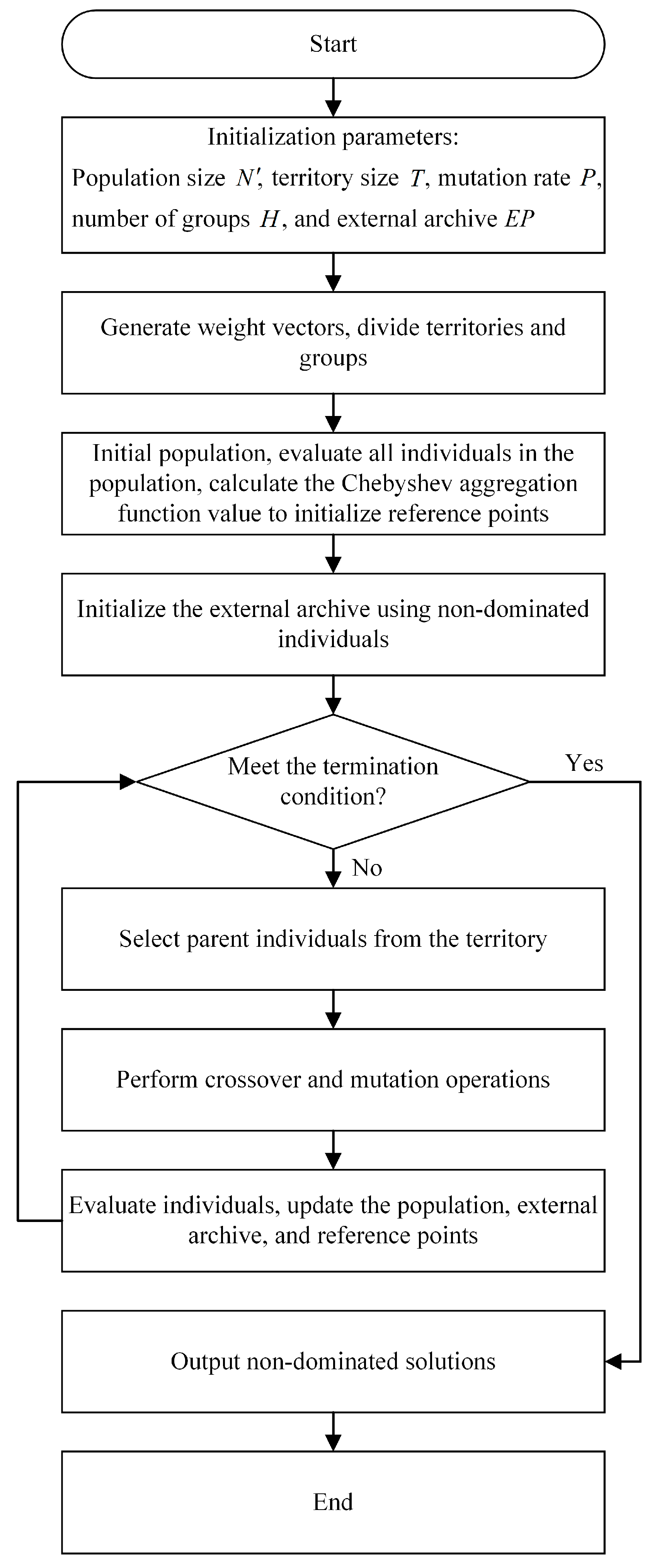
3.2. The Algorithm of MOEA/D

The optimization strategy of MOEA/D decomposes complex multi-objective optimization problems into multiple single-objective subproblems and optimizes them in parallel. Each subproblem is associated with a specific weight vector, enabling the algorithm to simultaneously optimize solutions in multiple directions. A key advantage of this approach is its ability to leverage neighborhood information, improving solution diversity and convergence efficiency by optimizing neighboring subproblems. This method greatly reduces the scope of ineffective searches, allowing for rapid convergence to the Pareto front within limited computational resources. Furthermore, the decomposition strategy of MOEA/D is highly scalable and can be seamlessly integrated with various optimization techniques, demonstrating exceptional robustness and stability, particularly in high-dimensional problems. Therefore, this paper adopts a strategy that combines MOEA/D with deep reinforcement learning to solve the PFSP.
Upon the completion of the training of the DRL-PFSP model in Section 3.1, it can quickly provide relatively good solutions for PFSP problems of different scales. In this section, we use these solutions as the initial population for the MOEA/D algorithm to further enhance the optimization capabilities of the algorithm, which is the DRL-MOEA/D method proposed in this paper. The fundamental procedure of the algorithm is outlined as follows:

3.2.1. Evaluation of Adaptation Values

In the MOEA/D framework, the Chebyshev aggregation function is typically employed to assess subproblems, as depicted in Equation (20).
g x | λ , z * = max λ b | f b x z b *
where λ = λ 1 , λ 2 , , λ b represents the weight vectors of the current subproblem, b represents the number of objectives in the multi-objective optimization problem, and z b * = min f b x | x X is the reference point.

3.2.2. Weight Vectors

In the MOEA/D algorithm, the weight vectors λ = λ 1 , λ 2 , , λ b typically adopt uniformly distributed weight vectors, which are generated based on a user-defined integer H , and H represents the subdivision level for each objective coordinate. Simultaneously, the weight vectors must not have duplicate values; hence, the number of weight vectors should meet the requirement of N = C H + b 1 b 1 . Furthermore, the weight vectors should satisfy Equations (21) and (22). In this paper, the weight vector λ is 0 , 1 , 0.01 , 0.99 , 0.02 , 0.98 , , 0.99 , 0.01 , 1 , 0 .
λ 1 + λ 2 + + λ b = 1
λ c 0 , 1 H , 2 H , , H H , c = 1 , 2 , , b

3.2.3. Neighborhood

In the MOEA/D algorithm framework, the concept of a neighborhood defines the specific scope for selection, evolution, and update operations within the population. The construction of neighborhoods is initialized by calculating the Euclidean distances between the weight vectors. For a specific weight vector λ c , the process of determining its neighborhood involves first calculating the Euclidean distances between λ c and all other weight vectors, and then selecting the T weight vectors with the smallest distances to form the neighborhood of λ c . The process of population evolution relies on a mutual collaboration and information exchange among subproblems within the neighborhood, thereby promoting the collaborative evolution of the entire population.

3.2.4. The Process of MOEA/D

The flowchart of MOEA/D is shown in Figure 5, and the specific process is as follows:
Step 1: Initialization.
  • Refine the initialization of N uniformly distributed reference weight vectors λ = λ 1 , λ 2 , , λ b , and then calculate the Euclidean geometric distance between vector λ c and each of these weight vectors. Subsequently, filter out the T weight vectors with the smallest Euclidean distances as the neighborhood of λ c and store the neighborhood information in the neighborhood matrix, i.e., the neighborhood of weight vector λ c is represented as B c = c 1 , c 2 , , c T , c = 1 , 2 , , N ;
  • Initialize population X = x 1 , x 2 , , x N based on the DRL-PFSP model, and calculate the fitness value F V c = F x c for each x c , c = 1 , 2 , , N ;
  • Initialize reference points z = z 1 , z 2 , , z b , where z d = min 1 c N f d x c , d = 1 , 2 , , b .
Step 2: Perform evolutionary operations on individual x c in the population, c = 1 , 2 , , N .
  • Select two random individuals from the neighborhood B c of individual x c , and generate a descendant individual y using crossover and mutation operations.
  • If f d y < z d , then update the reference point z d = f d y , d = 1 , 2 , , b .
  • Update the neighborhood solutions, that is, for t B c , if g y | λ t , z g x t | λ t , z , then x t = y , F V t = F y .
Step 3: If the termination condition is met, the algorithm stops and outputs the optimal solution; otherwise, continue with step 2.

3.3. The Energy-Saving Strategy

In Section 3.2, we successfully obtained the relatively optimal solution for the completion time of the PFSP. To further optimize energy consumption, this paper proposes a novel energy-saving strategy aimed at effectively reducing overall energy consumption while keeping the longest completion time unchanged. As indicated by the objective function (4), the energy consumption of a machine is composed of the energy used during processing and the energy consumed while idle. Specifically, the processing energy consumption E p r o is the product of the job processing time and the machine’s processing power, while the idle energy consumption E i d is the product of the machine’s idle time and the idle power of the machine. Given the fixed processing time of jobs, the machine’s processing power, and the machine’s idle power, the key to reducing energy consumption lies in minimizing the machine’s idle time to decrease idle energy consumption, thereby achieving the goal of reducing the overall energy consumption of all machines.
Therefore, this paper proposes a job postponement strategy to reduce the idle time of machines. However, not all jobs are suitable for delayed processing, and those jobs can be postponed, but must meet the following two conditions: (1) The completion time of the job that can be postponed must be earlier than the start time of the job immediately following it, i.e., C i j < S i + 1 j ; and (2) the completion time of the current operation for the job that can be postponed must be earlier than the start time of the next operation, i.e., C i j < S i j + 1 . Specifically, the process begins by traversing all jobs on machine M m in reverse order based on their start or completion times, performing the postponement operation on jobs that meet condition (1). Subsequently, the same approach is used to traverse all jobs on machine M m 1 , applying the postponement operation to jobs that satisfy both condition (1) and condition (2). This process continues in the same manner until the traversal reaches the jobs on machine M 1 , at which point the loop ends.
To vividly and concretely understand the energy-saving strategy proposed in this paper, we take the job sequence depicted in Figure 1 as an example to elaborate. First, all jobs on Machine M 5 are traversed in reverse order based on their start or completion times, and jobs 4, 5, 2, 1, and 3 are found to meet condition (1), so the postponement operation is performed on these jobs. Next, using the same method, the jobs on Machine M 4 are traversed, and jobs 4, 5, 2, 1, and 3 are found to meet both condition (1) and condition (2), so the postponement operation is applied to these jobs again. This process continues with the jobs on Machine M 3 and Machine M 2 , where each job is checked to see if it meets both condition (1) and condition (2); if they do, the postponement is applied. Finally, the loop ends after traversing the jobs on Machine M 1 . The enhanced Gantt chart, as depicted in Figure 6b, is contrasted with Figure 6a to illustrate that the job postponement strategy has greatly reduced the total idle time of the machines, consequently diminishing the overall energy consumption. Consequently, the energy-saving strategy presented in this paper effectively reduces the overall energy consumption.

4. Numerical Experiments

4.1. Experimental Settings

To validate the effectiveness and practicality of the proposed GDRL-MOEA/D framework and the energy-saving strategy for solving the GPFSP in this paper, a comprehensive series of experiments is conducted. All experiments are developed using Python 3.7 on an Intel Core i7 CPU/2.8 GHz PC and a GTX 2060.
To train the DRL-PFSP model in this study, 100,000 instances are randomly generated in each epoch, with each instance having 50 jobs and the number of machines being an integer in the range of 5 ,   20 . The processing times of jobs are generated stochastically from a uniform distribution across the [0, 1] interval. This strategy not only significantly improves the computational efficiency of the model, but also enhances its versatility in accommodating PFSPs of diverse scales, thereby significantly bolstering the model’s robustness. The entire training process of the model requires approximately 300 h. To assess the scheduling performance of the proposed GDRL-MOEA/D algorithm, this paper conducts comparative experiments with the MOEA/D, NSGA-II, marine predators algorithm (MPA) [60], sparrow search algorithm (SSA) [61], artificial hummingbird algorithm (AHA) [62], and seagull optimization algorithm (SOA) [63]. All algorithms are tested using instances with the number of jobs n belonging to set 50 , 100 , 150 , 200 and the number of machines m belonging to set 5 , 6 , 7 , 10 , 15 , 20 . Therefore, each algorithm corresponds to 24 different combinations of n , m scale variations. For each scale, the processing times of jobs are randomly generated, adhering to a uniform distribution ranging from 0 to 1. And all comparison algorithms are run independently 15 times. Additionally, to streamline the computation of energy consumption, the machines’ processing power is set to 1, while the idle power is assigned a value of 0.2.
To maintain equity in the comparative analysis of algorithms, the parameters for the benchmark algorithms are configured as follows: NSGA-II is assigned a population size of 100, a crossover rate of 0.7, a mutation rate of 0.05, and a total of 200 iterations; MOEA/D is equipped with a population size of 100, a neighborhood size of 15, a mutation rate of 0.05, a weight vector parameter of 99, and a total of 200 iterations; MPA is assigned a population size of 100, an initial fish aggregation device influence value of 0.2, a fast movement probability of 0.5, and a total of 200 iterations; SSA is configured with a population size of 100, an alert threshold of 0.6, a discoverers proportion of 0.7, an aware sparrows proportion of 0.2, and a total of 200 iterations; AHA is equipped with a population size of 100 and a total of 200 iterations; and SOA is assigned a population size of 100 and a total of 200 iterations.
The relative percentage deviation is used as the evaluation metric for all algorithms, as shown in Equations (23) and (24), where R P D 1 and R P D 2 represent the maximum percentage deviation of the maximum completion time and the maximum percentage deviation of the energy consumption, respectively. C max * denotes the best C max obtained by all compared algorithms, C max a lg is the average value of C max obtained by algorithm a lg , E * is the best E obtained by all compared algorithms, and E a lg represents the average value of E obtained by algorithm a lg .
R P D 1 = C max a lg C max * / C max * × 100
R P D 2 = E a lg E * / E * × 100

4.2. Parameter Settings of the DRL-PFSP Model

During the training process, the parameters of the network model are set as shown in Table 3. The variable D i n p u t represents the dimensionality of the input data. The decoder employs a single-layer GRU RNN with a hidden layer size of 128 units. Similarly, the critic network is also configured with a hidden layer size of 128 units. Both the actor and critic networks are trained using the Adam optimizer, with a learning rate η of 0.0001 and a batch size of 256 for each training iteration.

4.3. Experimental Results and Discussions

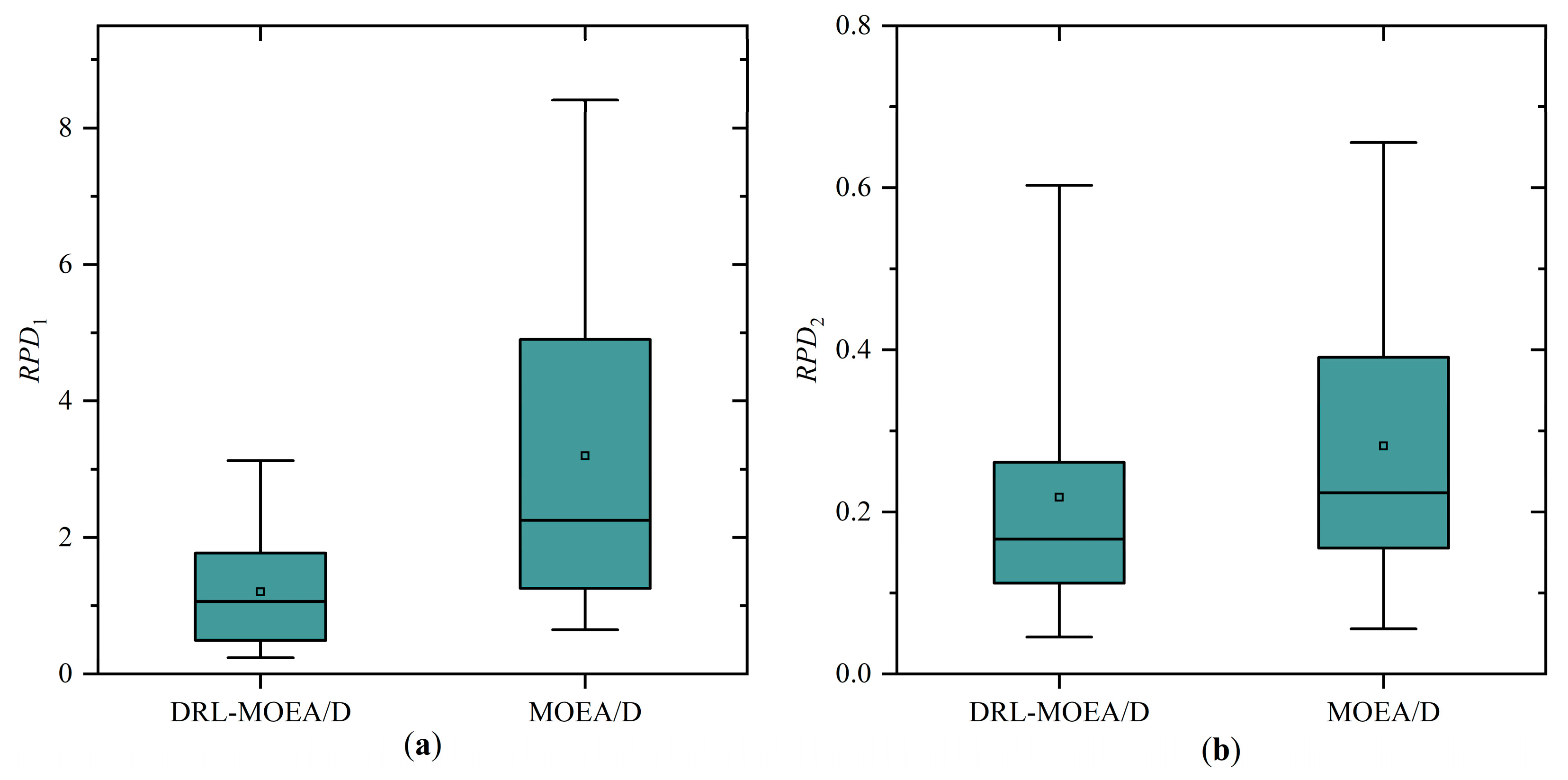
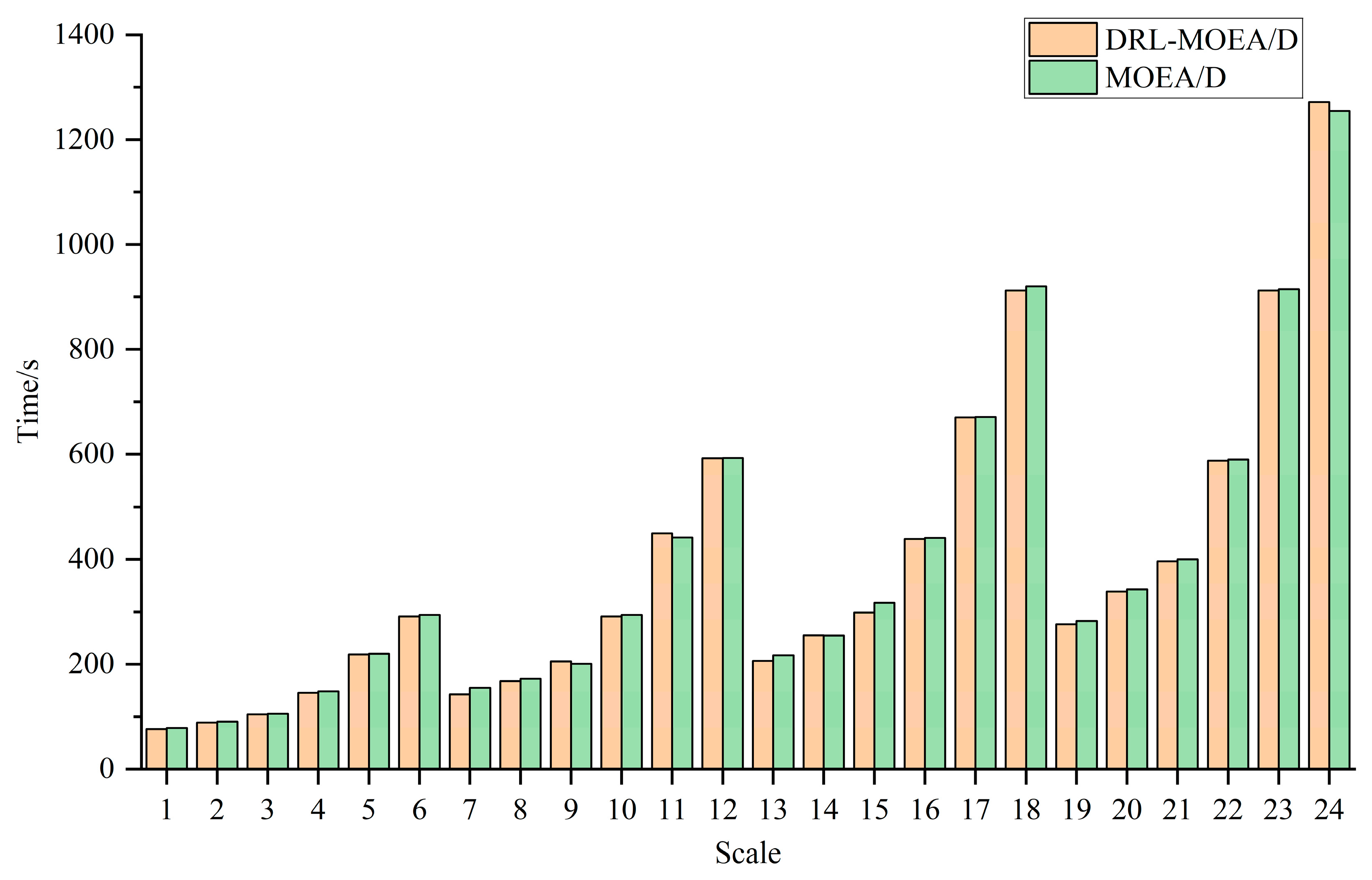
4.3.1. The Effectiveness of Initializing the Population Based on DRL-PFSP

In Section 3.1, we employ an end-to-end deep reinforcement learning method to model the PFSP and train the model using the actor–critic algorithm. Once training is complete, the model is capable of swiftly generating solutions based on the scale of the PFSP, which are then used as the initial population for the MOEA/D algorithm, thereby forming the DRL-MOEA/D method. To validate the effectiveness of this strategy, this section compares it with the traditional MOEA/D algorithm in terms of the maximum completion time and energy consumption objectives. The averages of the RPD value and computation time for each algorithm across different problem scales are presented in Table 4. To more intuitively observe the comparison results, a graphical representation of the outcomes for both methods has been created, as shown in Figure 7 and Figure 8. The numbers 1 to 24 in Figure 8 on the x-axis represent different scales from (50, 5) to (200, 20).
As indicated in Table 4 and Figure 7, the DRL-MOEA/D algorithm has a lower average RPD value for both the maximum completion time and energy consumption across all scales compared to the MOEA/D algorithm, demonstrating that the DRL-MOEA/D algorithm outperforms the MOEA/D algorithm in terms of performance. Furthermore, as observed in Table 4 and Figure 8, the computational times of the two algorithms are relatively close, but the solution time of the DRL-MOEA/D algorithm is generally lower than that of the MOEA/D algorithm across most problem scales. This is because the DRL-PFSP model, once trained, can quickly produce relatively optimized solutions to serve as the initial population for the DRL-MOEA/D algorithm. Therefore, it is evident that using the DRL-PFSP model to enhance the initial population strategy of MOEA/D not only significantly improves the solution quality of the MOEA/D algorithm, but also achieves a slight increase in solution speed.

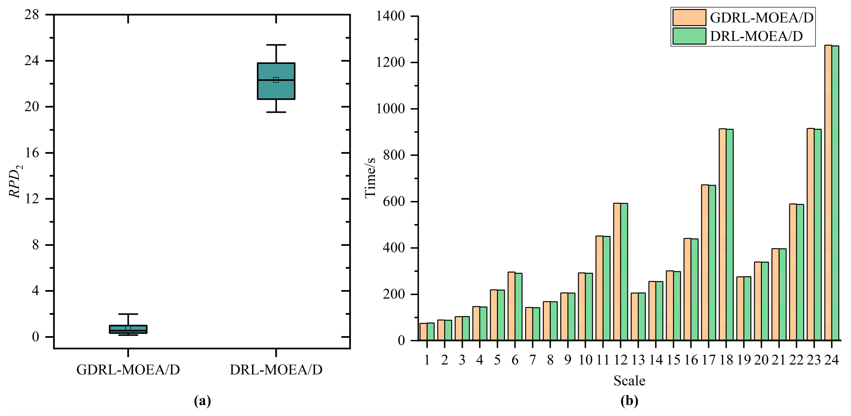
4.3.2. The Effectiveness of the Energy-Saving Strategy

In Section 3.3, to further optimize the energy consumption objective, we proposed a job postponement strategy for energy saving. The purpose of this section is to validate the effectiveness of this strategy. A comparative experiment is conducted between the GDRL-MOEA/D algorithm with the energy-saving strategy and the DRL-MOEA/D algorithm without the energy-saving strategy, as discussed in the previous section, focusing on the energy consumption objective. The average energy consumption RPD value and average computation time for both algorithms are presented in Table 5 and Figure 9. As shown in Table 5 and Figure 9a, the GDRL-MOEA/D algorithm significantly outperforms the DRL-MOEA/D algorithm in terms of average energy consumption RPD value across all problem scales. Additionally, Table 5 and Figure 9b indicate that the performance difference in solution time between the two algorithms is minimal, with both being relatively close, although the DRL-MOEA/D algorithm has a slight edge.

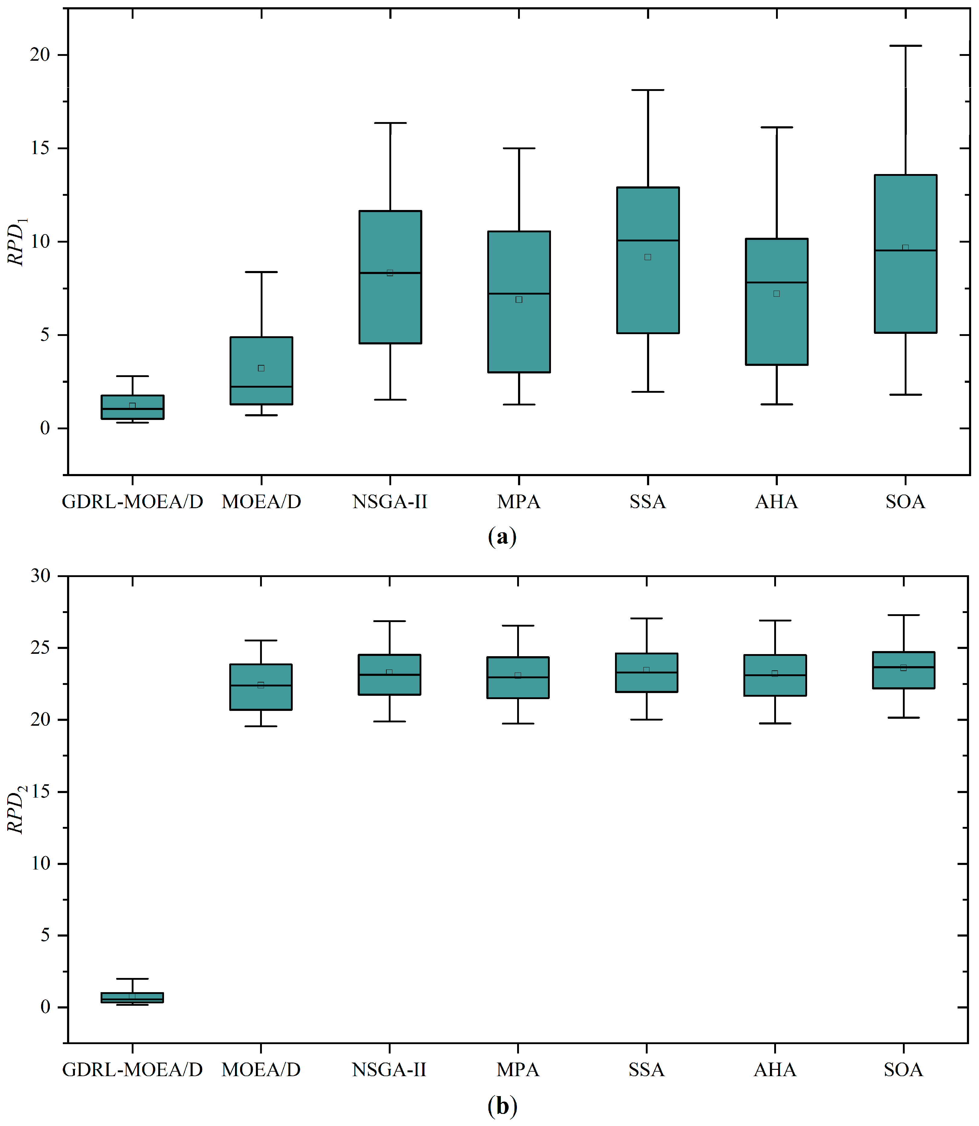
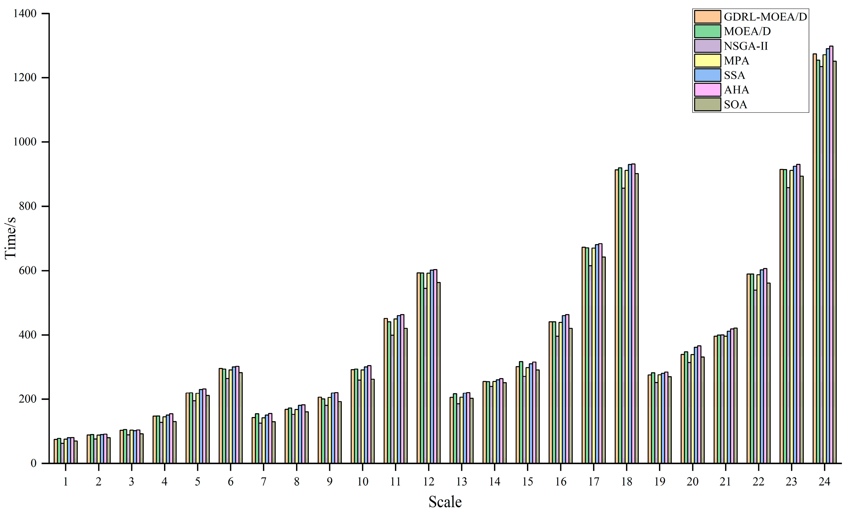
4.3.3. Comparison with Other Algorithms

To further validate the performance of the proposed GDRL-MOEA/D algorithm, this section conducts comparative experiments with the classic multi-objective optimization algorithms MOEA/D and NSGA-II, as well as the latest metaheuristic algorithms MPA, SSA, AHA, and SOA. These algorithms are briefly summarized in Table 6.
Based on the descriptions of the algorithms compared in Table 6, it is evident that these algorithms exhibit good robustness and global search capabilities in solving complex problems such as production scheduling and multi-objective decision making, effectively finding high-quality solutions. Therefore, selecting these algorithms for comparison with the GDRL-MOEA/D algorithm proposed in this paper can provide a more comprehensive validation of the performance of GDRL-MOEA/D.
The results of the comparative experiments for the algorithms are shown in Table 7, Table 8, and Figure 10 and Figure 11. As is shown in Table 7 and the boxplot of Figure 10, the GDRL-MOEAD algorithm achieved the best RPD1 and RPD2 indicators across all test sets compared to the other six algorithms, particularly excelling in the RPD2 indicator, where its performance far exceeded that of the other algorithms, verifying the effectiveness of the energy-saving strategy proposed in this paper. Additionally, Table 7 and Figure 10 demonstrate that the MOEA/D algorithm outperformed the other algorithms in both RPD1 and RPD2, further validating the rationale behind combining the DRL and MOEA/D algorithms. Among the remaining five algorithms, MPA and AHA showed relatively close performances in RPD1, outperforming the other three algorithms, while in RPD2, the five algorithms exhibited similar performances. A bar chart was created based on the computation time data of the seven algorithms for the different problem sizes shown in Table 8, as illustrated in Figure 11. As visually depicted in Figure 11, the computation times of all seven algorithms increased as the problem size grew, and the solution speeds of the algorithms were relatively close at each scale, with the NSGA2 algorithm performing slightly better. Overall, the computation times of all the algorithms were within an acceptable range.
In summary, although the GDRL-MOEA/D algorithm proposed in this paper is relatively close to other algorithms in terms of solution speed for different scales of PFSP, it consistently outperforms other algorithms in solution quality. Therefore, by improving the initial population strategy of MOEA/D through deep reinforcement learning and combining it with the proposed energy-saving strategy, this paper not only enhances the solution performance of MOEA/D to a certain extent, but also slightly increases its solution speed.

5. Conclusions and Future Work

This paper focuses on solving the green permutation flow shop scheduling problem with energy consumption consideration (GPFSP), aiming to minimize the maximum completion time and the total energy consumption of machines. A novel solution method combining the end-to-end deep reinforcement learning technique with the MOEA/D algorithm (DRL-MOEA/D) is proposed. Firstly, an end-to-end DRL method is employed to model the PFSP as a sequence-to-sequence model (DRL-PFSP), which is then trained using the actor–critic algorithm. This model does not rely on high-quality labels and can directly output scheduling solutions for PFSP of various scales once it has been trained. Secondly, considering the advantages of the MOEA/D algorithm in solution quality, robustness, and adaptability to complex problems, the solutions output by the DRL-PFSP model are used as the initial solutions for the MOEA/D algorithm, thereby enhancing the quality of the final solutions produced by the MOEA/D algorithm. Moreover, to more effectively optimize the energy consumption target, a job postponement energy-saving strategy is proposed, which reduces machine idle time without increasing the maximum completion time, thus further optimizing energy consumption. Finally, through a series of simulation experiments, the proposed GDRL-MOEA/D algorithm is compared with the unimproved MOEA/D, NSGA-II, MPA, SSA, AHA, and SOA. The experimental results indicate that the GDRL-MOEA/D algorithm outperforms MOEA/D, NSGA-II, MPA, SSA, AHA, and SOA in solution quality. These algorithms exhibit similar solution speeds across different scales, with the speed differences falling within an acceptable range.
However, the GDRL-MOEA/D method proposed in this paper is designed to solve static GPFSP without considering the dynamic factors that GPFSP may encounter in the actual production process, such as machine failures, sudden order arrivals, and random order arrivals. Therefore, in future work, we will design an DRL algorithm that takes into account the dynamic factors of the workshop and extend the algorithm to solve other types of workshop scheduling problems, such as the parallel machine scheduling problem, the flexible flow shop scheduling problem, and the distributed flow shop scheduling problem.

Author Contributions

Conceptualization, Y.L. and Y.Y.; methodology, Y.L.; software, Y.L.; validation, Y.L.; data curation, Y.L.; writing—original draft preparation, Y.L.; writing—review and editing, Y.Y., A.S., and Y.C.; visualization, Y.L.; supervision, Y.Y., A.S., Y.C., and Y.W.; project administration, Y.Y. and Y.C. All authors have read and agreed to the published version of the manuscript.

Funding

This research was funded by the National Natural Science Foundation of China (72361032), the Xinjiang Autonomous Region Key R&D Project (2022B01057-2) and the Xinjiang Autonomous Region Natural Science Foundation-Youth Fund (2023D01C177).

Data Availability Statement

The data are contained within the article.

Conflicts of Interest

The authors declare no conflicts of interest.

References

  1. McMahon, G.; Burton, P. Flow-shop scheduling with the branch-and-bound method. Oper. Res. 1967, 15, 473–481. [Google Scholar] [CrossRef]
  2. Yavuz, M.; Tufekci, S. Dynamic programming solution to the batching problem in just-in-time flow-shops. Comput. Ind. Eng. 2006, 51, 416–432. [Google Scholar] [CrossRef]
  3. Ronconi, D.P.; Birgin, E.G. Mixed-Integer Programming Models for Flowshop Scheduling Problems Minimizing the Total Earliness and Tardiness. In Just-in-Time Systems; Springer: Berlin/Heidelberg, Germany, 2012; pp. 91–105. [Google Scholar]
  4. Campbell, H.G.; Dudek, R.A.; Smith, M.L. A heuristic algorithm for the n job, m machine sequencing problem. Manag. Sci. 1970, 16, B-630–B-637. [Google Scholar]
  5. Gupta, J.N. A functional heuristic algorithm for the flowshop scheduling problem. J. Oper. Res. Soc. 1971, 22, 39–47. [Google Scholar] [CrossRef]
  6. Nawaz, M.; Enscore, E.E., Jr.; Ham, I. A heuristic algorithm for the m-machine, n-job flow-shop sequencing problem. Omega 1983, 11, 91–95. [Google Scholar] [CrossRef]
  7. Johnson, S.M. Optimal two-and three-stage production schedules with setup times included. Nav. Res. Logist. Q. 1954, 1, 61–68. [Google Scholar] [CrossRef]
  8. Puka, R.; Duda, J.; Stawowy, A.; Skalna, I. N-NEH+ algorithm for solving permutation flow shop problems. Comput. Oper. Res. 2021, 132, 105296. [Google Scholar] [CrossRef]
  9. Puka, R.; Skalna, I.; Duda, J.; Stawowy, A. Deterministic constructive vN-NEH+ algorithm to solve permutation flow shop scheduling problem with makespan criterion. Comput. Oper. Res. 2024, 162, 106473. [Google Scholar] [CrossRef]
  10. Puka, R.; Skalna, I.; Łamasz, B.; Duda, J.; Stawowy, A. Deterministic method for input sequence modification in NEH-based algorithms. IEEE Access 2024, 12, 68940–68953. [Google Scholar] [CrossRef]
  11. Zhang, J.; Dao, S.D.; Zhang, W.; Goh, M.; Yu, G.; Jin, Y.; Liu, W. A new job priority rule for the NEH-based heuristic to minimize makespan in permutation flowshops. Eng. Optim. 2023, 55, 1296–1315. [Google Scholar] [CrossRef]
  12. Zheng, J.; Wang, Y. A hybrid bat algorithm for solving the three-stage distributed assembly permutation flowshop scheduling problem. Appl. Sci. 2021, 11, 10102. [Google Scholar] [CrossRef]
  13. Chen, S.; Zheng, J. Hybrid grey wolf optimizer for solving permutation flow shop scheduling problem. Concurr. Comput. Pract. Exp. 2024, 36, e7942. [Google Scholar] [CrossRef]
  14. Tian, S.; Li, X.; Wan, J.; Zhang, Y. A novel cuckoo search algorithm for solving permutation flowshop scheduling problems. In Proceedings of the 2021 IEEE International Conference on Recent Advances in Systems Science and Engineering (RASSE), Tainan, Taiwan, 7–10 November 2021; pp. 1–8. [Google Scholar]
  15. Khurshid, B.; Maqsood, S.; Omair, M.; Sarkar, B.; Ahmad, I.; Muhammad, K. An improved evolution strategy hybridization with simulated annealing for permutation flow shop scheduling problems. IEEE Access 2021, 9, 94505–94522. [Google Scholar] [CrossRef]
  16. Razali, F.; Nawawi, A. Optimization of Permutation Flowshop Schedulling Problem (PFSP) using First Sequence Artificial Bee Colony (FSABC) Algorithm. Prog. Eng. Appl. Technol. 2024, 5, 369–377. [Google Scholar]
  17. Qin, X.; Fang, Z.; Zhang, Z. Hybrid symbiotic organisms search algorithm for permutation flow shop scheduling problem. J. Zhejiang Univer. Eng. Sci. 2020, 54, 712–721. [Google Scholar]
  18. Rui, Z.; Jun, L.; Xingsheng, G. Mixed No-Idle Permutation Flow Shop Scheduling Problem Based on Multi-Objective Discrete Sine Optimization Algorithm. J. East China Univ. Sci. Technol. 2022, 48, 76–86. [Google Scholar]
  19. Yan, H.; Tang, W.; Yao, B. Permutation flow-shop scheduling problem based on new hybrid crow search algorithm. Comput. Integr. Manuf. Syst. 2024, 30, 1834. [Google Scholar]
  20. Yang, L. Unsupervised machine learning and image recognition model application in English part-of-speech feature learning under the open platform environment. Soft Comput. 2023, 27, 10013–10023. [Google Scholar] [CrossRef]
  21. Mohi-Ud-Din, G.; Marnerides, A.K.; Shi, Q.; Dobbins, C.; MacDermott, A. Deep COLA: A deep competitive learning algorithm for future home energy management systems. IEEE Trans. Emerg. Top. Comput. Intell. 2020, 5, 860–870. [Google Scholar] [CrossRef]
  22. Dudhane, A.; Patil, P.W.; Murala, S. An end-to-end network for image de-hazing and beyond. IEEE Trans. Emerg. Top. Comput. Intell. 2020, 6, 159–170. [Google Scholar] [CrossRef]
  23. Bai, X.; Wang, X.; Liu, X.; Liu, Q.; Song, J.; Sebe, N.; Kim, B. Explainable deep learning for efficient and robust pattern recognition: A survey of recent developments. Pattern Recognit. 2021, 120, 108102. [Google Scholar] [CrossRef]
  24. Aurangzeb, K.; Javeed, K.; Alhussein, M.; Rida, I.; Haider, S.I.; Parashar, A. Deep Learning Approach for Hand Gesture Recognition: Applications in Deaf Communication and Healthcare. Comput. Mater. Contin. 2024, 78, 127–144. [Google Scholar] [CrossRef]
  25. Malik, N.; Altaf, S.; Tariq, M.U.; Ahmed, A.; Babar, M. A Deep Learning Based Sentiment Analytic Model for the Prediction of Traffic Accidents. Comput. Mater. Contin. 2023, 77, 1599–1615. [Google Scholar] [CrossRef]
  26. Vinyals, O.; Fortunato, M.; Jaitly, N. Pointer networks. arXiv 2015, arXiv:1506.03134. [Google Scholar]
  27. Ling, Z.; Tao, X.; Zhang, Y.; Chen, X. Solving optimization problems through fully convolutional networks: An application to the traveling salesman problem. IEEE Trans. Syst. Man Cybern. Syst. 2020, 51, 7475–7485. [Google Scholar] [CrossRef]
  28. Zhang, R.; Zhang, C.; Cao, Z.; Song, W.; Tan, P.S.; Zhang, J.; Wen, B.; Dauwels, J. Learning to solve multiple-TSP with time window and rejections via deep reinforcement learning. IEEE Trans. Intell. Transp. Syst. 2022, 24, 1325–1336. [Google Scholar] [CrossRef]
  29. Luo, J.; Li, C.; Fan, Q.; Liu, Y. A graph convolutional encoder and multi-head attention decoder network for TSP via reinforcement learning. Eng. Appl. Artif. Intell. 2022, 112, 104848. [Google Scholar] [CrossRef]
  30. Bogyrbayeva, A.; Yoon, T.; Ko, H.; Lim, S.; Yun, H.; Kwon, C. A deep reinforcement learning approach for solving the traveling salesman problem with drone. Transp. Res. Part C Emerg. Technol. 2023, 148, 103981. [Google Scholar] [CrossRef]
  31. Gao, H.; Zhou, X.; Xu, X.; Lan, Y.; Xiao, Y. AMARL: An attention-based multiagent reinforcement learning approach to the min-max multiple traveling salesmen problem. IEEE Trans. Neural Netw. Learn. Syst. 2023, 35, 9758–9772. [Google Scholar] [CrossRef]
  32. Wang, Q.; Hao, Y.; Zhang, J. Generative inverse reinforcement learning for learning 2-opt heuristics without extrinsic rewards in routing problems. J. King Saud Univ.-Comput. Inf. Sci. 2023, 35, 101787. [Google Scholar] [CrossRef]
  33. Pan, W.; Liu, S.Q. Deep reinforcement learning for the dynamic and uncertain vehicle routing problem. Appl. Intell. 2023, 53, 405–422. [Google Scholar] [CrossRef]
  34. Wang, Q.; Hao, Y. Routing optimization with Monte Carlo Tree Search-based multi-agent reinforcement learning. Appl. Intell. 2023, 53, 25881–25896. [Google Scholar] [CrossRef]
  35. Xu, Y.; Fang, M.; Chen, L.; Xu, G.; Du, Y.; Zhang, C. Reinforcement learning with multiple relational attention for solving vehicle routing problems. IEEE Trans. Cybern. 2021, 52, 11107–11120. [Google Scholar] [CrossRef] [PubMed]
  36. Zhao, J.; Mao, M.; Zhao, X.; Zou, J. A hybrid of deep reinforcement learning and local search for the vehicle routing problems. IEEE Trans. Intell. Transp. Syst. 2020, 22, 7208–7218. [Google Scholar] [CrossRef]
  37. Si, J.; Li, X.; Gao, L.; Li, P. An efficient and adaptive design of reinforcement learning environment to solve job shop scheduling problem with soft actor-critic algorithm. Int. J. Prod. Res. 2024, 1–16. [Google Scholar] [CrossRef]
  38. Chen, R.; Li, W.; Yang, H. A deep reinforcement learning framework based on an attention mechanism and disjunctive graph embedding for the job-shop scheduling problem. IEEE Trans. Ind. Inform. 2022, 19, 1322–1331. [Google Scholar] [CrossRef]
  39. Shao, C.; Yu, Z.; Tang, J.; Li, Z.; Zhou, B.; Wu, D.; Duan, J. Research on flexible job-shop scheduling problem based on variation-reinforcement learning. J. Intell. Fuzzy Syst. 2024, 1–15. [Google Scholar] [CrossRef]
  40. Han, B.; Yang, J. A deep reinforcement learning based solution for flexible job shop scheduling problem. Int. J. Simul. Model. 2021, 20, 375–386. [Google Scholar] [CrossRef]
  41. Yuan, E.; Wang, L.; Cheng, S.; Song, S.; Fan, W.; Li, Y. Solving flexible job shop scheduling problems via deep reinforcement learning. Expert Syst. Appl. 2024, 245, 123019. [Google Scholar] [CrossRef]
  42. Wan, L.; Cui, X.; Zhao, H.; Li, C.; Wang, Z. An effective deep actor-critic reinforcement learning method for solving the flexible job shop scheduling problem. Neural Comput. Appl. 2024, 36, 11877–11899. [Google Scholar] [CrossRef]
  43. Peng, S.; Xiong, G.; Yang, J.; Shen, Z.; Tamir, T.S.; Tao, Z.; Han, Y.; Wang, F.-Y. Multi-Agent Reinforcement Learning for Extended Flexible Job Shop Scheduling. Machines 2023, 12, 8. [Google Scholar] [CrossRef]
  44. Wu, X.; Yan, X.; Guan, D.; Wei, M. A deep reinforcement learning model for dynamic job-shop scheduling problem with uncertain processing time. Eng. Appl. Artif. Intell. 2024, 131, 107790. [Google Scholar] [CrossRef]
  45. Liu, R.; Piplani, R.; Toro, C. A deep multi-agent reinforcement learning approach to solve dynamic job shop scheduling problem. Comput. Oper. Res. 2023, 159, 106294. [Google Scholar] [CrossRef]
  46. Gebreyesus, G.; Fellek, G.; Farid, A.; Fujimura, S.; Yoshie, O. Gated-Attention Model with Reinforcement Learning for Solving Dynamic Job Shop Scheduling Problem. IEEJ Trans. Electr. Electron. Eng. 2023, 18, 932–944. [Google Scholar] [CrossRef]
  47. Wu, X.; Yan, X. A spatial pyramid pooling-based deep reinforcement learning model for dynamic job-shop scheduling problem. Comput. Oper. Res. 2023, 160, 106401. [Google Scholar] [CrossRef]
  48. Su, C.; Zhang, C.; Xia, D.; Han, B.; Wang, C.; Chen, G.; Xie, L. Evolution strategies-based optimized graph reinforcement learning for solving dynamic job shop scheduling problem. Appl. Soft Comput. 2023, 145, 110596. [Google Scholar] [CrossRef]
  49. Liu, C.-L.; Huang, T.-H. Dynamic job-shop scheduling problems using graph neural network and deep reinforcement learning. IEEE Trans. Syst. Man Cybern. Syst. 2023, 53, 6836–6848. [Google Scholar] [CrossRef]
  50. Zhu, H.; Tao, S.; Gui, Y.; Cai, Q. Research on an Adaptive Real-Time Scheduling Method of Dynamic Job-Shop Based on Reinforcement Learning. Machines 2022, 10, 1078. [Google Scholar] [CrossRef]
  51. Tiacci, L.; Rossi, A. A discrete event simulator to implement deep reinforcement learning for the dynamic flexible job shop scheduling problem. Simul. Model. Pract. Theory 2024, 134, 102948. [Google Scholar] [CrossRef]
  52. Zhang, L.; Feng, Y.; Xiao, Q.; Xu, Y.; Li, D.; Yang, D.; Yang, Z. Deep reinforcement learning for dynamic flexible job shop scheduling problem considering variable processing times. J. Manuf. Syst. 2023, 71, 257–273. [Google Scholar] [CrossRef]
  53. Chang, J.; Yu, D.; Zhou, Z.; He, W.; Zhang, L. Hierarchical reinforcement learning for multi-objective real-time flexible scheduling in a smart shop floor. Machines 2022, 10, 1195. [Google Scholar] [CrossRef]
  54. Zhou, T.; Luo, L.; Ji, S.; He, Y. A Reinforcement Learning Approach to Robust Scheduling of Permutation Flow Shop. Biomimetics 2023, 8, 478. [Google Scholar] [CrossRef] [PubMed]
  55. Pan, Z.; Wang, L.; Wang, J.; Lu, J. Deep reinforcement learning based optimization algorithm for permutation flow-shop scheduling. IEEE Trans. Emerg. Top. Comput. Intell. 2021, 7, 983–994. [Google Scholar] [CrossRef]
  56. Wang, Z.; Cai, B.; Li, J.; Yang, D.; Zhao, Y.; Xie, H. Solving non-permutation flow-shop scheduling problem via a novel deep reinforcement learning approach. Comput. Oper. Res. 2023, 151, 106095. [Google Scholar] [CrossRef]
  57. Jiang, E.-D.; Wang, L. An improved multi-objective evolutionary algorithm based on decomposition for energy-efficient permutation flow shop scheduling problem with sequence-dependent setup time. Int. J. Prod. Res. 2019, 57, 1756–1771. [Google Scholar] [CrossRef]
  58. Rossit, D.G.; Nesmachnow, S.; Rossit, D.A. A Multiobjective Evolutionary Algorithm based on Decomposition for a flow shop scheduling problem in the context of Industry 4.0. Int. J. Math. Eng. Manag. Sci. 2022, 7, 433–454. [Google Scholar]
  59. Nazari, M.; Oroojlooy, A.; Snyder, L.; Takác, M. Reinforcement learning for solving the vehicle routing problem. arXiv 2018, arXiv:1802.04240. [Google Scholar]
  60. Faramarzi, A.; Heidarinejad, M.; Mirjalili, S.; Gandomi, A.H. Marine Predators Algorithm: A nature-inspired metaheuristic. Expert Syst. Appl. 2020, 152, 113377. [Google Scholar] [CrossRef]
  61. Xue, J.; Shen, B. A novel swarm intelligence optimization approach: Sparrow search algorithm. Syst. Sci. Control Eng. 2020, 8, 22–34. [Google Scholar] [CrossRef]
  62. Zhao, W.; Wang, L.; Mirjalili, S. Artificial hummingbird algorithm: A new bio-inspired optimizer with its engineering applications. Comput. Methods Appl. Mech. Eng. 2022, 388, 114194. [Google Scholar] [CrossRef]
  63. Dhiman, G.; Kumar, V. Seagull optimization algorithm: Theory and its applications for large-scale industrial engineering problems. Knowl.-Based Syst. 2019, 165, 169–196. [Google Scholar] [CrossRef]
Figure 1. Gantt chart of the instance for PFSP.
Machines 12 00721 g001
Figure 2. The framework of the GDRL-MOEA/D algorithm.
Machines 12 00721 g002
Figure 3. The structure for the DRL-PFSP. The red arrow indicates that the selected job at the current time step is job 2.
Machines 12 00721 g003
Figure 4. The input structure of the encoder network.
Machines 12 00721 g004
Figure 5. The flowchart of MOEA/D.
Machines 12 00721 g005
Figure 6. An example of the energy-saving strategy for PFSP. (a) represents the Gantt chart without using the energy-saving strategy; (b) represents the Gantt chart after using the energy-saving strategy.
Machines 12 00721 g006
Figure 7. The boxplot of the average RPD value. (a) represents the boxplot of the average RPD value for the maximum completion time; (b) represents the boxplot of the average RPD value for the energy consumption.
Machines 12 00721 g007
Figure 8. The computation time of two algorithms for each scale.
Machines 12 00721 g008
Figure 9. The boxplot of the average RPD value and the average computation time of algorithms. (a) represents the boxplot of the average RPD value; (b) represents the computation time of two algorithms for each scale.
Machines 12 00721 g009
Figure 10. The boxplot of the average RPD value. (a) represents the boxplot of the average RPD value for the maximum completion time; (b) represents the boxplot of the average RPD value for energy consumption.
Machines 12 00721 g010
Figure 11. The computation times of seven algorithms for each scale.
Machines 12 00721 g011
Table 1. Existing methods for solving various shop scheduling problems.
ReferencesType of ProblemObjectivesApproachApproach Type
[1]PFSPMakespanBranch and boundExact algorithms
[2]PFSPMakespanDynamic programming
[3]PFSPMakespanInteger programming
[4]PFSPMakespanCampbell Dudek Smith algorithmHeuristic methods
[5]PFSPMakespanGupta algorithm
[6,7,8,9,10,11]PFSPMakespanNawaz Enscore Ham algorithm
[12]PFSPMakespanHybrid bat optimization algorithmMetaheuristic methods
[13]PFSPMakespanHybrid grey wolf algorithm
[14]PFSPMakespan, total energy consumptionCuckoo search algorithm
[15]PFSPMakespanHybrid Evolution Strategy
[16]PFSPMakespanArtificial Bee Colony algorithm
[17]PFSPMakespanHybrid cooperative coevolutionary search algorithm
[18]PFSPMakespan, maximum tardinessDiscrete sine optimization method
[19]PFSPMakespanHybrid crow search algorithm
[37]JSSPMakespanSoft actor–critic algorithmReinforcement learning methods
[38]JSSPMakespanDeep reinforcement learning
[39]FJSSPMakespanHybrid deep reinforcement learning
[40]FJSSPMakespanDeep reinforcement learning
[41]FJSSPMakespanDeep reinforcement learning
[42]FJSSPMakespanDeep actor–critic reinforcement learning
[43]FJSSPMakespanMulti-agent reinforcement learning
[44]DJSSPMakespanDeep reinforcement learning
[45]DJSSPMakespanDeep multi-agent reinforcement learning
[46]DJSSPMakespanGated-attention model with reinforcement learning
[47]DJSSPMakespanDeep reinforcement learning
[48]DJSSPMakespanGraph reinforcement learning
[49]DJSSPMakespanGraph neural network and deep reinforcement learning
[50]DJSSPMakespanDeep reinforcement learning
[51]DFJSSPMakespanDeep reinforcement learning
[52]DFJSSPMakespanProximal Policy Optimization algorithm
[53]DFJSSPMakespanThe combination of a double deep Q-network (DDQN) and a dueling DDQN
[54]PFSPMakespanDeep reinforcement learning
[55]PFSPMakespanDeep reinforcement learning
[56]PFSPMakespanDeep reinforcement learning
Table 2. Descriptions of notations.
NotationsDefinition
n The total number of jobs
m The total number of machines or the total number of job operations
i , i i and i   represent   the   different   indices   of   jobs ,   i , i = 1 , 2 , , n
j The   index   of   operations ,   j = 1 , 2 , , m
k The   index   of   machines ,   k = 1 , 2 , , m
q i The number of operations for job i
O i j The   j t h operation of job i
p i j The processing time of job i   on   machine   M j
C i The completion time of job i
S i j The   start   time   of   operation   O i j
F i j The   completion   time   of   operation   O i j
T i j k The   processing   time   of   operation   O i j   on   machine   M k , k is the index of machines
a i j k The   load   unit   energy   consumption   of   operation   O i j   on   machine   M k , k is the index of machines
b k The   idle   unit   energy   consumption   of   machine   M k , k is the index of machines
E The total energy consumption of all machines
C max The maximum completion time
X i j k X i j k = 1   if   the   operation   O i j   is   processed   on   machine   M k ;   otherwise ,   X i j k = 0 , k is the index of machines
X i i X i i = 1 if job i is the immediate predecessor operation of job i ;   otherwise ,   X i i = 0
v a ,   v b ,   W a ,   W b The learnable parameters of the DRL-PFSP model
e The context vectors output by the encoder
d t The decoding vector from the decoder at time step t
a t The “attention” mask for the inputs at time step t
b t The context vector at time step t
P ρ t + 1 | ρ 1 , ρ 2 , , ρ t , X t The   highest   probability   value   of   the   job ,   ρ 1 , ρ 2 , , ρ t , represents the jobs that have been selected at time step t ;   X t represents the jobs available at time step t
θ The network parameters of the actor network
ϕ The network parameters of the critic network
R a The actual reward value yielded by the actor network, for in-stance, a
N The total number of training instances
V X 0 a ; ϕ The expected reward of the critic network for each instance
x The individuals of the population
N The population size
λ = λ 1 , λ 2 , , λ b The weight vectors of the current subproblem, where b is the number of objectives for the problem
z * The reference points
H The subdivision level for each objective coordinate
g x | λ , z * The Chebyshev aggregation function; x represents an individual in the population
R P D 1 The maximum percentage deviation of the maximum completion time
R P D 2 The maximum percentage deviation of the energy consumption
C max * The   best   C max obtained by all compared algorithms
C max a lg The   average   value   of   C max   obtained   by   algorithm   a lg
E * The best E obtained by all compared algorithms
E a lg The average value of E   obtained   by   algorithm   a lg
Table 3. The parameter settings of the model.
Actor Network (Pointer Network)Critic Network
Encoder: 1D-Conv( D i n p u t , 128, kernel size = 1, stride = 1)1D-Conv ( D i n p u t , 128, kernel size = 1, stride = 1)
1D-Conv (128, 20, kernel size = 1, stride = 1)
Decoder: GRU (hidden size = 128, number of layers = 1)
Attention (No hyper parameters)
1D-Conv (20, 20, kernel size = 1, stride = 1)
1D-Conv (20, 1, kernel size = 1, stride = 1)
Table 4. The average RPD value for each algorithm at each scale.
(n, m)The Average RPD Value for Each AlgorithmThe Computation Time of Algorithm/s
DRL-MOEA/DMOEA/DDRL-MOEA/DMOEA/D
RPD1RPD2RPD1RPD2
(50, 5)0.51740.60320.64800.655976.230278.3117
(50, 6)1.10570.11151.72870.177588.521490.2976
(50, 7)1.99050.21663.64390.2200104.2893105.8324
(50, 10)1.70880.12982.29660.4152145.2546148.1882
(50, 15)2.51230.56628.40980.5736218.6872219.9746
(50, 20)3.12920.59786.60610.6120291.0637294.0099
(100, 5)0.26830.13291.11070.1424142.1222154.5248
(100, 6)0.55150.19390.91470.1727168.0217172.2160
(100, 7)1.41650.17182.21100.1727205.3689200.6013
(100, 10)1.59760.18724.24940.2198291.2315293.9304
(100, 15)1.83480.28425.07510.3575450.0200441.8432
(100, 20)2.21500.44927.20530.4710592.2356592.6549
(150, 5)0.32710.11420.86540.1200206.2297216.773
(150, 6)0.47950.10931.26980.1323255.2442254.7261
(150, 7)1.01680.06752.02410.2564298.3484316.9811
(150, 10)0.42520.16071.23710.1682439.0293441.1019
(150, 15)1.33550.15444.73220.3040669.9642670.6341
(150, 20)1.67960.29395.15430.3693912.1419920.1188
(200, 5)0.54830.05170.84840.0765276.1188282.2372
(200, 6)0.23850.04581.32820.0558338.6582342.7295
(200, 7)0.50960.06381.62520.0943396.4272400.0306
(200, 10)0.46510.11282.64570.2268587.6343589.5134
(200, 15)0.98840.23874.69160.4121912.2259914.6555
(200, 20)2.01330.17966.24650.35291271.59791254.9765
AVG1.20310.21823.19870.2816389.0278391.5359
Table 5. The average RPD value and average computation time for each algorithm at each scale.
(n, m)The Average RPD Value for Each
Algorithm
The Computation Time of Each
Algorithm/s
GDRL-MOEA/DDRL-MOEA/DGDRL-MOEA/DDRL-MOEA/D
RPD2RPD2
(50, 5)1.6924 20.126175.125476.2302
(50, 6)1.6876 24.318089.245288.5214
(50, 7)1.9866 24.5283103.5411104.2893
(50, 10)0.9362 19.7679147.3512145.2546
(50, 15)0.8797 24.7655219.5412218.6872
(50, 20)0.4857 20.6822295.6234291.0637
(100, 5)0.4237 19.5342143.2415142.1222
(100, 6)1.4500 23.6355168.6145168.0217
(100, 7)0.3360 22.3653206.1235205.3689
(100, 10)0.3590 20.6560292.2514291.2315
(100, 15)0.6011 25.3751451.3547450.0200
(100, 20)0.3944 21.6173593.1045592.2356
(150, 5)0.9851 20.5960205.6841206.2297
(150, 6)1.2060 21.8462255.4562255.2442
(150, 7)0.7356 23.7286301.2514298.3484
(150, 10)0.3196 22.4336441.0145439.0293
(150, 15)0.3807 22.2747672.5241669.9642
(150, 20)0.1680 23.8685913.8121912.1419
(200, 5)0.9916 19.6915275.6581276.1188
(200, 6)0.4009 21.2566339.2514338.6582
(200, 7)0.7289 22.9484396.5412396.4272
(200, 10)0.2848 21.9042589.5418587.6343
(200, 15)0.2600 25.3070915.2564912.2259
(200, 20)0.1676 22.81831274.45141271.5979
AVG0.7442 22.3352 390.2317389.5359
Table 6. Brief summary of algorithms.
AlgorithmsDescriptionsCharacteristicApplication Scenarios
NSGA-IIAn advanced genetic algorithm for solving multi-objective optimization problems, which introduces improvements such as fast non-dominated sorting, crowding distance estimation, and elitist strategies based on NSGA, significantly enhancing the algorithm’s efficiency and solution quality.NSGA-II achieves precise sorting of solutions with lower computational complexity and maintains population diversity through crowding distance.Production scheduling, engineering design, path planning, power system optimization, etc.
MPAA metaheuristic algorithm designed based on the predatory behavior of marine predators, which simulates the dynamic behavior of predators during the processes of hunting and migration to balance global search and local exploitation.MPA excels at handling optimization problems with complex search spaces, effectively avoiding local optima and demonstrating strong global optimization capabilities.Engineering design, logistics optimization, production scheduling, etc.
SSAA metaheuristic algorithm based on sparrow foraging behavior, aimed at solving complex optimization problems by simulating the collaboration and decision-making mechanisms of sparrows during the foraging process.SSA is simple in structure and easy to implement, with good optimization ability and convergence speed.Production scheduling, resource allocation, etc.
AHAA metaheuristic algorithm that simulates behaviors such as guiding foraging, area foraging, and migratory foraging of hummingbirds.AHA demonstrates high adaptability, allowing it to dynamically adjust search strategies based on the scale and complexity of the problem, exhibiting good flexibility and robustness.Production scheduling, path planning, multi-objective decision making, etc.
SOAA metaheuristic algorithm based on the migration and predatory behavior of seagulls, aimed at solving complex global optimization problems.SOA is characterized by simplicity and ease of implementation, strong global search capabilities, and broad applicability.Engineering optimization, data mining, production scheduling, image processing, etc.
Table 7. The average RPD value for each algorithm at each scale.
(n, m)The Average RPD Value for Each Algorithm
GDRL-MOEA/DMOEA/DNSGA-IIMPASSAAHASOA
RPD1RPD2RPD1RPD2RPD1RPD2RPD1RPD2RPD1RPD2RPD1RPD2RPD1RPD2
(50, 5)0.53491.69240.695220.19424.049820.87033.114420.70636.005621.20364.113520.80557.294921.3956
(50, 7)0.72691.68761.741624.40014.664624.83792.840924.63835.227724.96393.060224.74686.993425.1091
(50, 10)2.12241.98663.636624.532511.503225.38969.122425.203713.933925.660711.027125.735015.972826.1701
(50, 15)1.72890.93622.264520.109310.451621.42957.589121.184311.212221.59839.897721.177412.812621.9546
(50, 20)2.48840.87978.377424.774616.357026.522114.999625.976418.145726.789916.132026.439120.496727.3059
(100, 5)2.79400.48576.550620.697913.890522.767612.522322.463414.122223.069410.802822.470714.295723.8263
(100, 6)0.49320.42371.092219.54544.441119.87942.880019.73335.047920.11752.995719.75425.558920.3161
(100, 7)0.35131.45000.859323.60945.079024.22413.340424.07385.148424.21053.407724.26494.683624.0524
(100, 10)1.25300.33602.208722.36648.097423.12237.363023.001710.304923.23998.694023.23079.402123.9177
(100, 15)1.68830.35904.249420.695312.667321.983810.600521.697113.305022.26349.803321.884013.456922.4374
(100, 20)1.37460.60115.040525.466713.151426.872011.526926.552814.117727.057411.960426.920114.353227.0540
(150, 5)2.14560.39447.189021.643713.690123.083512.134322.909114.373123.364012.838023.126615.022823.3508
(150, 6)0.55950.98511.356320.60303.316520.83772.515620.74104.336620.88752.854620.74963.151220.8535
(150, 7)0.49321.20601.267321.87424.087622.24642.835822.15853.745022.27953.396922.20034.302522.4164
(150, 10)1.06790.73562.022923.75724.937624.11183.831224.03264.859124.19313.436824.18814.658124.3320
(150, 15)0.60390.31961.233722.44286.042723.16584.881822.93356.910123.23865.237023.16307.458423.3205
(150, 20)1.50000.38074.720122.457211.114523.49949.083523.033311.982723.71748.342223.091012.174923.8704
(200, 5)1.78730.16805.154323.961711.601225.261510.697825.412812.329525.505810.159525.432513.690325.5540
(200, 6)0.46530.99160.832519.72131.529320.00451.272919.89211.950320.02211.284219.84861.809320.1448
(200, 7)0.30320.40091.300121.26882.606821.50871.849121.32933.353621.57231.992421.45493.993021.8319
(200, 10)0.43830.72891.634922.98605.519923.45553.698523.15766.279723.46934.558623.07606.571223.5114
(200, 15)0.55980.28482.614822.04318.549722.81287.061822.52059.838622.98717.279122.49299.658122.9751
(200, 20)1.02070.26004.646025.523710.628926.64268.996926.561410.976826.77889.538426.634311.289826.7975
AVG2.08760.16766.236523.030711.679424.139610.496523.899112.515724.284310.133823.988912.842624.2816
Table 8. The average computation times of three algorithms for each scale.
(n, m)The Computation Time of Each Algorithm/s
GDRL-MOEA/DMOEA/DNSGA-IIMPASSAAHASOA
(50, 5)75.125478.311763.438676.230280.412581.125270.5412
(50, 6)89.245290.297676.779788.521490.541291.524180.4224
(50, 7)103.5411105.832489.2609104.2893102.4125104.632192.4125
(50, 10)147.3512148.1881128.1632145.2546150.5412154.5214130.5418
(50, 15)219.5412219.9746194.9998218.6872230.4512232.1745211.2156
(50, 20)295.6234294.0099264.4712291.0637300.4124302.4512282.9541
(100, 5)143.2415154.5248125.7052142.1222150.5416155.5412130.1445
(100, 6)168.6145172.2160152.7174168.0217180.9841182.4152160.7841
(100, 7)206.1235200.6013180.8117205.3689219.5412220.7451192.5412
(100, 10)292.2514293.9304259.8535291.2315300.7451304.5415262.3562
(100, 15)451.3547441.1938399.5518450.0200460.4152463.1278420.7412
(100, 20)593.1045592.6549544.2545592.2356601.5471603.4985563.6482
(150, 5)205.6841216.7729185.8298206.2297218.8471220.7894202.3541
(150, 6)255.4562254.7261240.0422255.2442260.4841264.3456251.5624
(150, 7)301.2514316.9811271.1553298.3484310.4514315.4514291.2481
(150, 10)441.0145441.1019396.4780439.0293460.4152463.3972420.7892
(150, 15)672.5241670.6341615.5960669.9642680.5123683.7456642.4874
(150, 20)913.8121920.1188856.0781912.1419930.2457932.1789902.1872
(200, 5)275.6581282.2372252.1723276.1188280.7451284.4152270.4671
(200, 6)339.2514347.0803314.1157338.6582361.5141365.8741331.3416
(200, 7)396.5412400.0306400.3811396.4272411.7452418.8415421.7412
(200, 10)589.5418589.5134539.3509587.6343602.4578606.7456561.5715
(200, 15)915.2564914.6555858.1994912.2259924.7451930.6481894.3251
(200, 20)1274.45141254.97651235.41911271.59791290.45141298.34581251.8413
AVG390.2317391.6902360.2011389.0278400.0483403.3782376.6758
Disclaimer/Publisher’s Note: The statements, opinions and data contained in all publications are solely those of the individual author(s) and contributor(s) and not of MDPI and/or the editor(s). MDPI and/or the editor(s) disclaim responsibility for any injury to people or property resulting from any ideas, methods, instructions or products referred to in the content.

