

Geometric Constraint Programming (GCP) Implemented Through GeoGebra to Study/Design Planar Linkages


Abstract
:1. Introduction
2. Materials and Methods
2.1. Building the Linkage and Generating Its Motion
2.1.1. Dyads
2.1.1.a. RRR Dyad
2.1.1.b. RRP Dyad
2.1.1.c. RPR Dyad
2.1.1.d PRP Dyad
2.1.1.e. RPP Dyad
2.1.2. Driving Links
2.1.2.a. Driving Link with Actuated R-pair
2.1.2.b. Driving Link with Actuated P-pair
2.1.3. Position Analysis’ Geometric Solution
2.2. Velocity and Acceleration Analyses’ Vector Diagrams
- -
- vP,g (aP,g) denotes the velocity (acceleration) of point P considered fixed to link g when measured from the frame;
- -
- vPR,g (aPR,g) denotes the velocity (acceleration) difference vP,g − vR,g (aP,g − aR,g);
- -
- vP,gm (aP,gm) denotes the velocity (acceleration) of point P considered fixed to link g when measured from link m;
- -
- ωg (αg) denotes the signed magnitude, positive if counterclockwise, of the angular velocity (acceleration) of link g when measured from the frame;
- -
- ωgm (αgm) denotes the signed magnitude, positive if counterclockwise, of the angular velocity (acceleration) of link g when measured from link m.
2.2.1. RRR Dyad
2.2.1.a. Vector Diagram of RRR Dyad’s Velocities
2.2.1.b. Vector Diagram of RRR Dyad’s Accelerations
2.2.2. RRP Dyad
2.2.2.a. Vector Diagram of RRP Dyad’s Velocities
2.2.2.b. Vector Diagram of RRP Dyad’s Acceleration
2.2.3. RPR Dyad
2.2.3.a. Vector Diagram of RPR Dyad’s Velocities
2.2.3.b. Vector Diagram of RPR Dyad’s Acceleration
2.2.4. PRP Dyad
2.2.4.a. Vector Diagram of PRP Dyad’s Velocities
2.2.4.b. Vector Diagram of PRP Dyad’s Acceleration
2.2.5. RPP Dyad
2.2.5.a. Vector Diagram of RPP Dyad’s Velocities
2.2.5.b. Vector Diagram of RPP Dyad’s Acceleration
2.3. Kinetostatics Analysis’ Vector Diagram
2.3.1. Free-Body Method
- (a)
- in the case of only two forces, if the two forces share the same line of action;
- (b)
- in the case of two forces and a pure moment, if the two forces have parallel and non-coincident lines of action;
- (c)
- in the case of only three forces, if the lines of action of the three forces share a common intersection point;
- (d)
- in the case of four forces, if the four forces, separated into two subsystems of two forces, gives two resultants, one for each subsystem, that are aligned along the line passing through the two intersections of the two lines of action of each subsystem.
2.3.2. Method Based on Active Load Diagrams
3. Results
3.1. Generation of Coupler Curves
3.2. Four-Bar Kinetostatics
3.3. Shaper Mechanism’s Kinematic Analysis
4. Discussion
5. Conclusions
Supplementary Materials
Author Contributions
Funding
Data Availability Statement
Conflicts of Interest
Appendix A
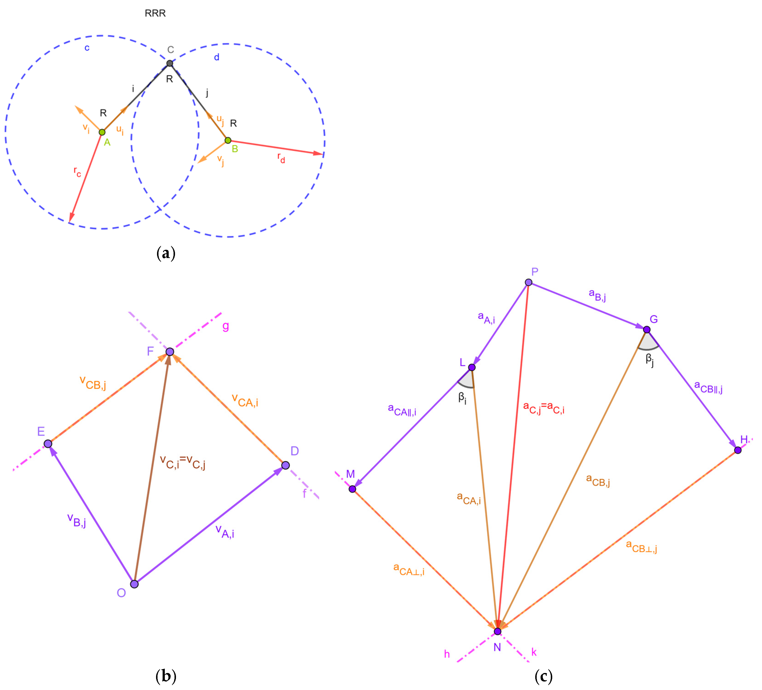
| A = (xA, yA) | (it generates point A and its coordinates as parameters of the object) |
| B = (xB, yB) | (it generates point B and its coordinates as parameters of the object) |
| c = Circle(A,rc) | (it generates the circle centered at A with radius rc and rc as parameter of the object) |
| d = Circle(B,rd) | (it generates the circle centered at B with radius rd and rd as parameter of the object) |
| C = Intersect(c,d) | (it locates point C at one intersection of circles c and d; here, the user must choose which intersection (i.e., dyad’s assembly mode) he/she is interested in) |
| i = Segment(A,C) | (it generates the segment representing link i) |
| j = Segment(B,C) | (it generates the segment representing link j) |
| ui = UnitVector(i) | (it generates the unit vector ui, parallel to segment i (i.e., AC (Figure 3a)) and located on it) |
| vi = UnitPerpendicularVector(i) | (it generates the unit vector vi, perpendicular to segment i) |
| uj = UnitVector(j) | (it generates the unit vector uj, parallel to segment j (i.e., BC (Figure 3a)) and located on it) |
| vj = UnitPerpendicularVector(j) | (it generates the unit vector vj, perpendicular to segment j) |
| O = (xO,yO) | (it generates point O and its coordinates as parameters of the object) |
| vA,i = Translate(Vector((vA,x,vA,y)),O) | (it generates the known velocity vector vA,i together with its components as parameters of the object and applies it to point O (see Figure 3b)) |
| D = O + vA,i | (it generates point D located at the point of the arrow representing vA,i) |
| f = Line(D, vi) | (it generates a line passing through D and parallel to vi, that is, parallel to the velocity difference vCA,i) |
| vB,j = Translate(Vector((vB,x,vB,y)),O) | (it generates the known velocity vector vB,j together with its components as parameters of the object and applies it to point O (see Figure 3b)) |
| E = O + vB,j | (it generates point E located at the point of the arrow representing vB,j) |
| g = Line(E, vj) | (it generates a line passing through E and parallel to vj, that is, parallel to the velocity difference vCB,j) |
| F = Intersect(f,g) | (it generates point F at the intersection of the two lines f and g (point F graphically solves Equation (3))) |
| vCA,i = Vector(D,F) | (it generates the arrow representing the velocity difference vCA,i) |
| vCB,j = Vector(E,F) | (it generates the arrow representing the velocity difference vCB,j) |
| vC,i = Vector(O,F) | (it generates the arrow representing the sought-after velocity vC,i(=vC,j)) |
| ωi = Dot(vCA,i,vi)/abs(C − A) | (it computes the signed magnitude, ωi, of the angular velocity of link i) |
| ωj = Dot(vCB,j,vj)/abs(C − B) | (it computes the signed magnitude, ωj, of the angular velocity of link j) |
| P = (xP,yP) | (it generates point P and its coordinates as parameters of the object) |
| aB,j = Translate(Vector((aB,x,aB,y)),P) | (it generates the known acceleration vector aB,j together with its components as parameters of the object and applies it to point P (see Figure 3c)) |
| G = P + aB,j | (it generates point G located at the point of the arrow representing aB,j) |
| aCB‖,j = Translate(Vector(−ωj2*|C − B|*ui), G) | (it computes the vector representing the acceleration component aCB‖,j and applies it to point G) |
| H = G + aCB‖,j | (it generates point H located at the point of the arrow representing aCB‖,j) |
| h = Line(H, vj) | (it generates a line passing through M and parallel to vj, that is, parallel to the acceleration component aCB⊥,j) |
| aA,i = Translate(Vector((aA,x,aA,y)),P) | (it generates the known acceleration vector aA,i together with its components as parameters of the object and applies it to point P (see Figure 3c)) |
| L = P + aA,i | (it generates point L located at the point of the arrow representing aA,i) |
| aCA‖,i = Translate(Vector(−ωi2*|C − A|*ui), L) | (it computes the vector representing the acceleration component aCA‖,i and applies it to point L) |
| M = L+ aCA‖,i | (it generates point M located at the point of the arrow representing aCA‖,i) |
| k = Line(M, vi) | (it generates a line passing through M and parallel to vi, that is, parallel to the acceleration component aCA⊥,i) |
| N = Intersect(k,h) | (it generates point N at the intersection of the two lines k and h (point N graphically solves Equation (4))) |
| aCA⊥,i = Vector(M,N) | (it generates the arrow representing the acceleration component aCA⊥,i) |
| aCB⊥,j = Vector(H,N) | (it generates the arrow representing the acceleration component aCB⊥,j) |
| aCA,i = Vector(L,N) | (it generates the arrow representing the acceleration difference aCA,i) |
| aCB,j = Vector(G,N) | (it generates the arrow representing the acceleration difference aCB,j) |
| aC,i = Vector(P,N) | (it generates the arrow representing the sought-after acceleration aC,i(=aC,j)) |
| βi = Angle(M,L,N) | (it generates the angle βi, which is the constant angle between aCA,i and (A − C)) |
| βj = Angle(N,G,H) | (it generates the angle βj, which is the constant angle between aCB,j and (B − C)) |
| αi = Dot(aCA⊥,i,vi)/abs(C − A) | (it computes the signed magnitude, αi, of the angular acceleration of link i) |
| αj = Dot(aCB⊥,j,vj)/abs(C − B) | (it computes the signed magnitude, αj, of the angular acceleration of link j) |
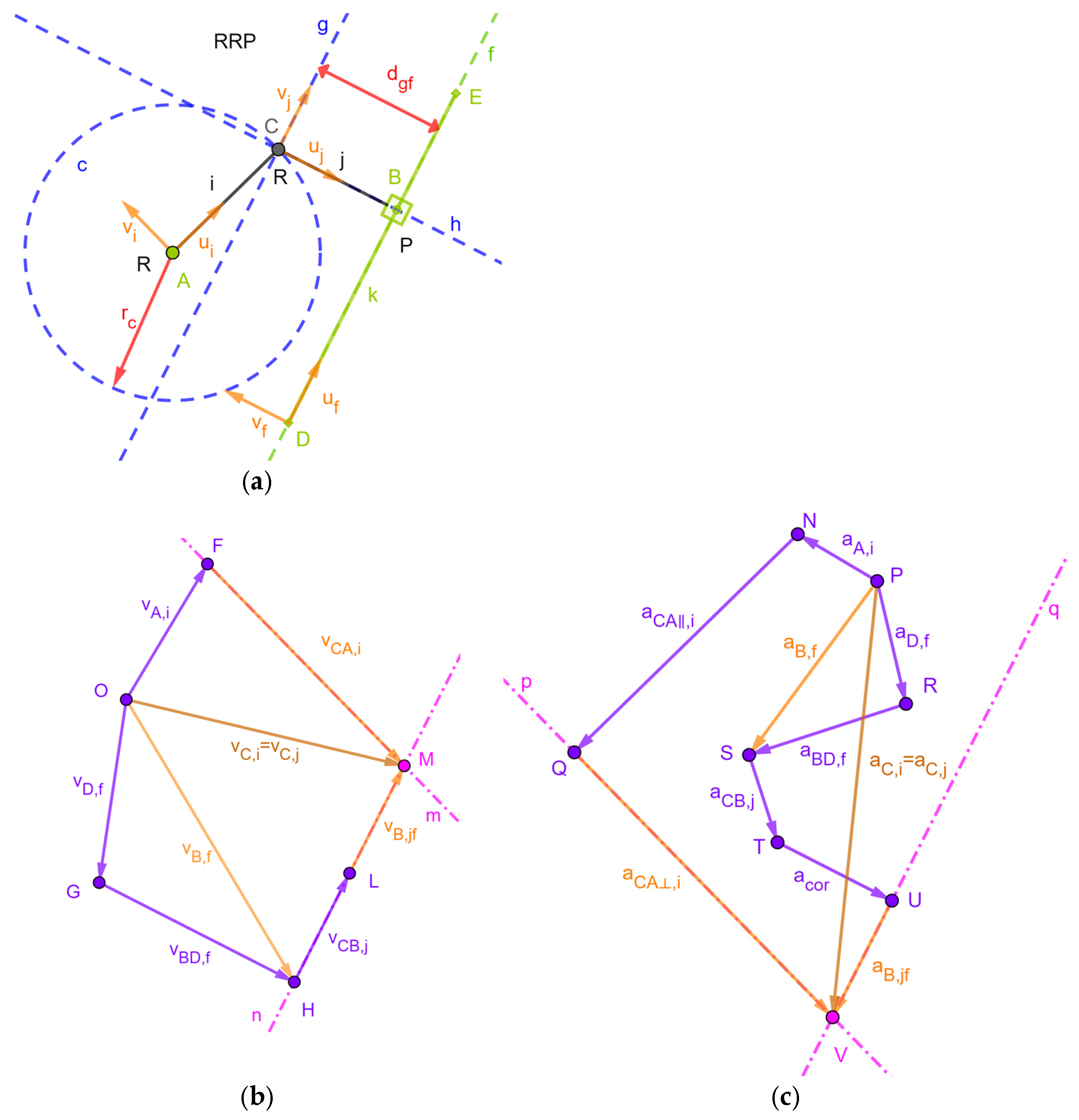
| A = (xA, yA) | (it generates point A and its coordinates as parameters of the object) |
| D = (xD, yD) | (it generates point D and its coordinates as parameters of the object) |
| f = Line(D,Vector((cos(θ),sin(θ)))) | (it generates line f passing through point D with the direction of the unit vector (cos(θ),sin(θ))T and the angle θ as a parameter of the object) |
| uf = UnitVector(f) | (it generates a unit vector parallel to line f and located on line f) |
| vf = UnitPerpendicularVector(f) | (it generates a unit vector perpendicular to line f) |
| c = Circle(A,rc) | (it generates the circle centered at A with radius rc and rc as parameters of the object) |
| g = Line(D + dgf*vf, uf) | (it generates a line parallel to line f whose distance from f is dgf and dgf as a parameter of the object) |
| C = Intersect(c,g) | (it locates point C at one intersection of circle c with line g; here, the user must choose which intersection (i.e., dyad’s assembly mode) he/she is interested in) |
| i = Segment(A,C) | (it generates the segment representing link i) |
| h = Line(C,vf) | (it generates a line passing through point C and perpendicular to line f) |
| B = Intersect(h,f) | (it generates the foot of the perpendicular from C to f) |
| j = Segment(B,C) | (it generates the segment representing link j) |
| Polygon(B + 0.5*aB*(vf − uf), B − 0.5*aB*(uf + vf), 4) | (it generates a regular polygon centered at B and with four sides (i.e., a square), parallel to uf or vf, whose length is aB and aB as a parameter of the object) |
| ui = UnitVector(i) | (it generates the unit vector ui, parallel to segment i (i.e., AC (Figure 4a) and located on it) |
| vi = UnitPerpendicularVector(i) | (it generates the unit vector vi, perpendicular to segment i) |
| uj = UnitVector(j) | (it generates the unit vector uj, parallel to segment j (i.e., BC (Figure 4a)) and located on it) |
| vj = UnitPerpendicularVector(j) | (it generates the unit vector vj, perpendicular to segment j) |
| O = (xO,yO) | (it generates point O and its coordinates as parameters of the object) |
| vA,i = Translate(Vector((vA,x,vA,y)),O) | (it generates the known velocity vector vA,i together with its components as parameters of the object and applies it to point O (see Figure 4b)) |
| F = O + vA,i | (it generates point F located at the point of the arrow representing vA,i) |
| m = Line(F, vi) | (it generates a line passing through F and parallel to vi, that is, parallel to the velocity difference vCA,i) |
| ωf = Slider(ωf,min, ωf,max, Δωf) | (it generates the variable ωf (necessary to assign the angular velocity, ωf, of line f) ranging from ωf,min to ωf,max with increment Δωf) |
| ωj = ωf | (it generates the dependent variable ωj (i.e., the signed magnitude of the angular velocity of link j)) |
| vD,f = Translate(Vector((vD,x,vD,y)),O) | (it generates the known velocity vector vD,f together with its components as parameters of the object and applies it to point O (see Figure 4b)) |
| G = O + vD,f | (it generates point G located at the point of the arrow representing vD,f) |
| vBD,f = Translate(Vector(ωf*|B − D|*vf),G) | (it generates the vector representing the velocity difference vBD,f and applies it to G (see Figure 4b)) |
| H = G + vBD,f | (it generates point H located at the point of the arrow representing vBD,f) |
| vB,f = Vector(O,H) | (it generates the arrow representing the velocity vB,f) |
| vCB,j = Translate(Vector(−ωj*|C − B|*vj),H) | (it generates the vector representing the velocity difference vCB,j and applies it to H (see Figure 4b)) |
| L = H+ vCB,j | (it generates point L located at the point of the arrow representing vCB,j) |
| n = Line(L, uf) | (it generates a line passing through L and parallel to uf, that is, parallel to the relative velocity vB,jf) |
| M = Intersect(m,n) | (it generates point M at the intersection of the two lines m and n (point M graphically solves Equation (5))) |
| vCA,i = Vector(F,M) | (it generates the arrow representing the velocity difference vCA,i) |
| vB,jf = Vector(L,M) | (it generates the arrow representing the relative velocity vB,jf) |
| vC,i = Vector(O,M) | (it generates the arrow representing the sought-after velocity vC,i(=vC,j)) |
| ωi = Dot(vCA,i,vi)/abs(C − A) | (it computes the signed magnitude, ωi, of the angular velocity of link i) |
| P = (xP,yP) | (it generates point P and its coordinates as parameters of the object) |
| aA,i = Translate(Vector((aA,x,aA,y)),P) | (it generates the known acceleration vector aA,i together with its components as parameters of the object and applies it to point P (see Figure 4c)) |
| N = P + aA,i | (it generates point N located at the point of the arrow representing aA,i) |
| aCA‖,i = Translate(Vector(−ωf2 *|C − A|*ui),N) | (it generates the vector representing the acceleration-difference component aCA‖,i and applies it to N (see Figure 4c)) |
| Q = N+ aCA‖,i | (it generates point Q located at the point of the arrow representing aCA‖,i) |
| p = Line(Q, vi) | (it generates a line passing through N and parallel to vi, that is, parallel to the acceleration difference component aCA⊥,i) |
| αf = Slider(αf,min, αf,max, Δαf) | (it generates the variable αf (necessary to assign the angular acceleration, αf, of line f) ranging from αf,min to αf,max with increment Δαf) |
| αj =αf | (it generates the dependent variable αj (i.e., the signed magnitude of the angular acceleration of link j)) |
| aD,f = Translate(Vector((aD,x,aD,y)),P) | (it generates the known acceleration vector aD,f together with its components as parameters of the object and applies it to point P (see Figure 4c)) |
| R = P + aD,f | (it generates point R located at the point of the arrow representing aD,f) |
| aBD,f = Translate(Vector((αf*vf − ωf2*uf)*|B − D|),R) | (it generates the vector representing the acceleration difference aBD,f and applies it to R (see Figure 4c)) |
| S = R + aBD,f | (it generates point S located at the point of the arrow representing aBD,f) |
| aB,f = Vector(P,S) | (it generates the arrow representing the velocity aB,f) |
| aCB,j = Translate(Vector(−(αj*vj − ωj2*uj)*|C − B|*vj),S) | (it generates the vector representing the acceleration difference aCB,j and applies it to S (see Figure 4c)) |
| T = S + aCB,j | (it generates point T located at the point of the arrow representing aCB,j) |
| acor = Translate(Vector(2*ωf*Dot(vB,jf,uf)*vf),T) | (it generates the vector representing the Coriolis acceleration acor and applies it to T (see Figure 4c)) |
| U = T + acor | (it generates point U located at the point of the arrow representing acor) |
| q = Line(U, uf) | (it generates a line passing through U and parallel to uf, that is, parallel to the relative acceleration aB,jf) |
| V = Intersect(p,q) | (it generates point V at the intersection of the two lines p and q (point V graphically solves Equation (6))) |
| aCA⊥,i = Vector(Q,V) | (it generates the arrow representing the acceleration difference component aCA⊥,i) |
| aB,jf = Vector(U,V) | (it generates the arrow representing the relative acceleration aB,jf) |
| aC,i = Vector(P,V) | (it generates the arrow representing the sought-after acceleration aC,i(=aC,j)) |
| αi = Dot(aCA⊥,i,vi)/abs(C − A) | (it computes the signed magnitude, αi, of the angular acceleration of link i) |
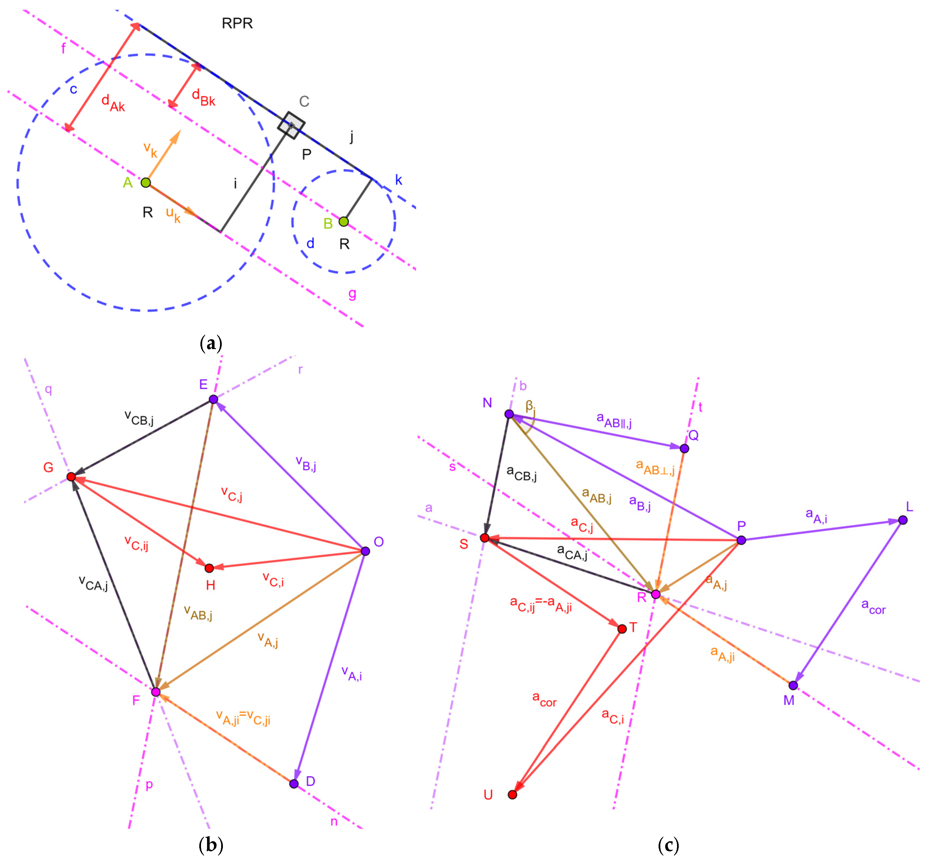
| A = (xA, yA) | (it generates point A and its coordinates as parameters of the object) |
| B = (xB, yB) | (it generates point B and its coordinates as parameters of the object) |
| c = Circle(A,dAk) | (it generates the circle centered at A with radius dAk and dAk as parameter of the object) |
| d = Circle(B,dBk) | (it generates the circle centered at B with radius dBk and dBk as parameter of the object) |
| k = Tangent(c,d) | (it generates line k as one of the possible common tangents to both the circles c and d; here, the user must choose which tangent (i.e., dyad’s assembly mode) he/she is interested in) |
| g = Line(A,k) | (it generates a line, named g, passing through point A and parallel to line k) |
| f = Line(B,k) | (it generates a line, named f, passing through point B and parallel to line k) |
| uk = UnitVector(g) | (it generates a unit vector parallel to line g and located on line g) |
| vk = UnitPerpendicularVector(g) | (it generates a unit vector perpendicular to line g) |
| i = Polyline(A,A + yk*uk,A + dAk*vk + yk*uk) | (it generates link i as a polyline with two sides, one parallel to line k with length yk and the other perpendicular to line k with length dAk, and yk as a parameter of the object) |
| j = Polyline(B,B + xk*uk,B + dBk*vk − xk*uk) | (it generates link j as a polyline with two sides, one parallel to line k with length xk and the other perpendicular to line k with length dBk, and xk as a parameter of the object) |
| C = Intersect(i,j) | (it generates the center, named C, of the P-pair slider as the intersection of the polylines i and j) |
| Polygon(C + 0.5*aC*(vk − uk), C − 0.5*aC*(uk + vk), 4) | (it generates a regular polygon centered at C and with four sides (i.e., a square), parallel to uk or vk, whose length is aC and aC as parameter of the object) |
| O = (xO,yO) | (it generates point O and its coordinates as parameters of the object) |
| vA,i = Translate(Vector((vA,x,vA,y)),O) | (it generates the known velocity vector vA,i together with its components as parameters of the object and applies it to point O (see Figure 5b)) |
| D = O + vA,i | (it generates point D located at the point of the arrow representing vA,i) |
| n = Line(D, uk) | (it generates a line passing through D and parallel to uk, that is, parallel to the relative velocity vA,ji (=vC,ji = −vC,ij)) |
| vB,j = Translate(Vector((vB,x,vB,y)),O) | (it generates the known velocity vector vB,j together with its components as parameters of the object and applies it to point O (see Figure 5b)) |
| E = O + vB,j | (it generates point E located at the point of the arrow representing vB,j) |
| p = Line(E, UnitPerpendicularVector(Segment(A,B))) | (it generates a line passing through E and perpendicular to segment AB, that is, parallel to the velocity difference vAB,j) |
| F = Intersect(p,n) | (it generates point F at the intersection of the two lines n and p (point F graphically solves Equation (8a))) |
| vA,ji = Vector(D,F) | (it generates the arrow representing the relative velocity vA,ji) |
| vAB,j = Vector(E,F) | (it generates the arrow representing the velocity difference vAB,j) |
| vA,j = Vector(O,F) | (it generates the arrow representing the velocity vA,j) |
| ωj = −Dot(vAB,j, UnitPerpendicularVector(Segment(A,B)))/abs(B − A) | (it computes the signed magnitude, ωj, of the angular velocity of link j) |
| ωi = ωj | (it generates the dependent variable ωi (i.e., the signed magnitude of the angular velocity of link i)) |
| q = Line(F, UnitPerpendicularVector(Segment(A,C))) | (it generates a line passing through F and perpendicular to segment AC, that is, parallel to vCA,j) |
| r = Line(E, UnitPerpendicularVector(Segment(B,C))) | (it generates a line passing through E and perpendicular to segment BC, that is, parallel to vCB,j) |
| G = Intersect(q,r) | (it generates point G at the intersection of the two lines q and r (point G graphically solves Equation (8b))) |
| vCA,j = Vector(F,G) | (it generates the arrow representing the velocity vCA,j) |
| vCB,j = Vector(E,G) | (it generates the arrow representing the velocity vCB,j) |
| vC,j = Vector(O,G) | (it generates the arrow representing the velocity vC,j) |
| vC,ij = Translate(−vA,ji,G) | (it generates the arrow representing vC,ij (=− vA,ji) and applies it at G) |
| vC,i = Translate(vC,j + vC,ij, O) | (it generates the arrow representing the sought-after velocity vC,i that solves Equation (8c)) |
| H = O + vC,i | (it generates point H located at the point of the arrow representing vC,i) |
| P = (xP,yP) | (it generates point P and its coordinates as parameters of the object) |
| aA,i = Translate(Vector((aA,x,aA,y)),P) | (it generates the known acceleration vector aA,i together with its components as parameters of the object and applies it to point P (see Figure 5c)) |
| L = P + aA,i | (it generates point L located at the point of the arrow representing aA,i) |
| acor = Translate(Vector(2*ωi*Dot(vA,ji, uk)*vk),L) | (it generates the vector representing the Coriolis acceleration acor and applies it to point L (see Figure 5c)) |
| M = L + acor | (it generates point M located at the point of the arrow representing acor) |
| s = Line(M, uk) | (it generates a line passing through M and parallel to uk, that is, parallel to the relative acceleration aA,ji (=aC,ji = −aC,ij)) |
| aB,j = Translate(Vector((aB,x,aB,y)),P) | (it generates the known acceleration vector aB,j together with its components as parameters of the object and applies it to point P (see Figure 5c)) |
| N = M + aB,j | (it generates point N located at the point of the arrow representing aB,j) |
| aAB‖,j = Translate(Vector(−ωj2*(A − B)),N) | (it computes aAB‖,j and generates the vector representing it applied at N (see Figure 5c)) |
| Q = N + aAB‖,j | (it generates point Q located at the point of the arrow representing aAB‖,j) |
| t = Line(Q,Vector(UnitPerpendicularVector(Segment(B,A)))) | (it generates a line passing through Q and perpendicular to segment BA, that is, parallel to aAB⊥,j) |
| R = Intersect(s,t) | (it generates point R at the intersection of the two lines s and t (point F graphically solves Equation (10a))) |
| aA,ji = Vector(M,R) | (it generates the arrow representing the relative acceleration aA,ji) |
| aAB⊥,j = Vector(Q,R) | (it generates the arrow representing the acceleration difference aAB⊥,j) |
| aAB,j = Vector(N,R) | (it generates the arrow representing the acceleration difference aAB,j) |
| aA,j = Vector(P,R) | (it generates the arrow representing the acceleration aA,j) |
| αj = Dot(aAB⊥,j, UnitPerpendicularVector(Segment(B,A)))/abs(B − A) | (it computes the signed magnitude, αj, of the angular acceleration of link j) |
| αi = αj | (it generates the dependent variable αi (i.e., the signed magnitude of the angular acceleration of link i) |
| βj = arctan(αj/ωj2) | (it computes the angle βj) |
| a = Rotate(Line(R, Segment(A,C)), − βj, R) | (it generates a line passing through R and parallel to aCA,j) |
| b = Rotate(Line(N, Segment(B,C)), − βj, N) | (it generates a line passing through N and parallel to aCB,j) |
| S = Intersect(a,b) | (it generates point S at the intersection of the two lines a and b (point S graphically solves Equation (10b))) |
| aCA,j = Vector(R,S) | (it generates the vector representing aCA,j) |
| aCB,j = Vector(N,S) | (it generates the vector representing aCB,j) |
| aC,j = Vector(P,S) | (it generates the vector representing aC,j) |
| aC,ij = Translate(−aA,ji, S) | (it generates the vector aC,ij (=− aA,ji) and applies it to S) |
| T = S+ aC,ij | (it generates point T located at the point of the arrow representing aC,ij) |
| U = T + acor | (it generates point U at the point of acor translated into T) |
| acor,translated = Vector(T,U) | (it generates a vector equal to acor translated into T) |
| aC,i = Vector(P,U) | (it generates the vector representing aC,I that solves Equation (10c)) |
| D = (xD, yD) | (it generates point D and its coordinates as parameters of the object) |
| f = Line(D,Vector((cos(θ),sin(θ)))) | (it generates line f passing through point D with the direction of the unit vector (cos(θ),sin(θ))T and the angle θ as parameter of the object) |
| E = (xE, yE) | (it generates point E and its coordinates as parameters of the object) |
| c= Line(E,Vector((cos(φ),sin(φ)))) | (it generates line c passing through point E with the direction of the unit vector (cos(φ),sin(φ))T and the angle φ as parameter of the object) |
| uf = UnitVector(f) | (it generates a unit vector parallel to line f and located on line f) |
| vf = UnitPerpendicularVector(f) | (it generates a unit vector perpendicular to line f) |
| uc = UnitVector(c) | (it generates a unit vector parallel to line c and located on line c) |
| vc = UnitPerpendicularVector(c) | (it generates a unit vector perpendicular to line c) |
| g = Line(D + dgf*vf, uf) | (it generates a line parallel to line f whose distance from f is dgf and dgf as parameter of the object) |
| n = Line(E − dcn*vc, uc) | (it generates a line parallel to line c whose distance from c is dcn and dcn as parameter of the object) |
| C = Intersect(n,g) | (it locates point C at the intersection of lines n and g) |
| h = Line(C,vf) | (it generates a line passing through point C and perpendicular to line f) |
| B = Intersect(h,f) | (it generates the foot of the perpendicular from C to line f) |
| j = Segment(B,C) | (it generates the segment representing link j) |
| Polygon(B + 0.5*aP*(vf − uf), B − 0.5*aP*(uf + vf), 4) | (it generates a regular polygon centered at B and with four sides (i.e., a square), parallel to uf or vf, whose length is aP and aP as a parameter of the object) |
| p = Line(C,vc) | (it generates a line passing through point C and perpendicular to line c) |
| A = Intersect(p,c) | (it generates the foot of the perpendicular from C to line c) |
| i = Segment(A,C) | (it generates the segment representing link i) |
| Polygon(A + 0.5*aP*(vc − uc), A − 0.5*aP*(uc + vc), 4) | (it generates a regular polygon centered at A and with four sides (i.e., a square), parallel to uc or vc, whose length is the already-defined parameter aP) |
| ui = UnitVector(i) | (it generates the unit vector ui, parallel to segment i (i.e., AC (Figure 6a) and located on it) |
| vi = UnitPerpendicularVector(i) | (it generates the unit vector vi, perpendicular to segment i) |
| uj = UnitVector(j) | (it generates the unit vector uj, parallel to segment j (i.e., BC (Figure 6a) and located on it) |
| vj = UnitPerpendicularVector(j) | (it generates the unit vector vj, perpendicular to segment j) |
| ωf = Slider(ωf,min, ωf,max, Δωf) | (it generates the variable ωf (necessary to assign the angular velocity, ωf, of line f) ranging from ωf,min to ωf,max with increment Δωf) |
| ωj = ωf | (it generates the dependent variable ωj (i.e., the signed magnitude of the angular velocity of link j)) |
| ωc = Slider(ωc,min, ωc,max, Δωc) | (it generates the variable ωc (necessary to assign the angular velocity, ωc, of line c) ranging from ωc,min to ωc,max with increment Δωc) |
| ωi = ωc | (it generates the dependent variable ωi (i.e., the signed magnitude of the angular velocity of link i)) |
| O = (xO,yO) | (it generates point O and its coordinates as parameters of the object) |
| vD,f = Translate(Vector((vD,x,vD,y)),O) | (it generates the known velocity vector vD,f together with its components as parameters of the object and applies it to point O (see Figure 6b)) |
| H = O + vD,f | (it generates point H located at the point of the arrow representing vD,f) |
| vBD,f = Translate(Vector(ωf*|B − D|*vf),H) | (it generates the vector representing the velocity difference vBD,f and applies it to G (see Figure 6b)) |
| L = H + vBD,f | (it generates point L located at the point of the arrow representing vBD,f) |
| vB,f = Vector(O,L) | (it generates the arrow representing the velocity vB,f) |
| vCB,j = Translate(Vector(−ωj*|C − B|*vj), L) | (it generates the vector representing the velocity difference vCB,j and applies it to L (see Figure 6b)) |
| M = H+ vCB,j | (it generates point M located at the point of the arrow representing vCB,j) |
| q = Line(M, uf) | (it generates a line passing through M and parallel to uf, that is, parallel to the relative velocity vB,jf) |
| vE,c = Translate(Vector((vE,x,vE,y)),O) | (it generates the known velocity vector vE,c together with its components as parameters of the object and applies it to point O (see Figure 6b)) |
| N = O + vE,c | (it generates point N located at the point of the arrow representing vE,c) |
| vAE,c = Translate(Vector(ωc*|A − E|*vc),N) | (it generates the vector representing the velocity difference vAE,c and applies it to N (see Figure 6b)) |
| Q = N + vAE,c | (it generates point Q located at the point of the arrow representing vAE,c) |
| vA,c = Vector(O,Q) | (it generates the arrow representing the velocity vA,c) |
| vCA,i = Translate(Vector(ωi*|C − A|*vi), Q) | (it generates the vector representing the velocity difference vCA,i and applies it to Q (see Figure 6b)) |
| R = Q+ vCA,i | (it generates point R located at the point of the arrow representing vCA,i) |
| r = Line(R, uc) | (it generates a line passing through R and parallel to uc, that is, parallel to the relative velocity vA,ic) |
| S = Intersect(r,q) | (it generates point S at the intersection of lines r and q (point S geometrically solves Equation (11))) |
| vA,ic = Vector(R,S) | (it generates the vector representing vA,ic) |
| vB,jf = Vector(M,S) | (it generates the vector representing vB,jf) |
| vC,j = Vector(O,S) | (it generates the vector representing the sought-after velocity vC,i (=vC,j)) |
| P = (xP,yP) | (it generates point P and its coordinates as parameters of the object) |
| αf = Slider(αf,min, αf,max, Δαf) | (it generates the variable αf (necessary to assign the angular acceleration, αf, of line f) ranging from αf,min to αf,max with increment Δαf) |
| αj =αf | (it generates the dependent variable αj (i.e., the signed magnitude of the angular acceleration of link j)) |
| aD,f = Translate(Vector((aD,x,aD,y)),P) | (it generates the known acceleration vector aD,f together with its components as parameters of the object and applies it to point P (see Figure 6c)) |
| T = P + aD,f | (it generates point T located at the point of the arrow representing aD,f) |
| aBD,f = Translate(Vector((αf*vf − ωf2*uf)*|B − D|),T) | (it generates the vector representing the acceleration difference aBD,f and applies it to T (see Figure 6c)) |
| U = T + aBD,f | (it generates point U located at the point of the arrow representing aBD,f) |
| aB,f = Vector(P,U) | (it generates the arrow representing the acceleration aB,f) |
| aCB,j = Translate(Vector(−(αj*vj − ωj2*uj)*|C − B|),U) | (it generates the vector representing the acceleration difference aCB,j and applies it to U (see Figure 6c)) |
| V = U + aCB,j | (it generates point V located at the point of the arrow representing aCB,j) |
| acor,f = Translate(Vector(2*ωf*Dot(vB,jf,uf)*vf),V) | (it generates the vector representing the Coriolis acceleration acor,f and applies it to V (see Figure 6c)) |
| W = V + acor,f | (it generates point W located at the point of the arrow representing acor,f) |
| s = Line(W, uf) | (it generates a line passing through W and parallel to uf, that is, parallel to the relative acceleration aB,jf) |
| αc = Slider(αc,min, αc,max, Δαc) | (it generates the variable αc (necessary to assign the angular acceleration, αc, of line c) ranging from αc,min to αc,max with increment Δαc) |
| αi =αc | (it generates the dependent variable αi (i.e., the signed magnitude of the angular acceleration of link i)) |
| aE,c = Translate(Vector((aE,x,aE,y)),P) | (it generates the known acceleration vector aE,c together with its components as parameters of the object and applies it to point P (see Figure 6c)) |
| T1 = P + aE,c | (it generates point T1 located at the point of the arrow representing aE,c) |
| aAE,c = Translate(Vector((αc*vc − ωc2*uc)*|A − E|),T1) | (it generates the vector representing the acceleration difference aAE,c and applies it to T1 (see Figure 6c)) |
| U1 = T1 + aAE,c | (it generates point U1 located at the point of the arrow representing aAE,c) |
| aA,c = Vector(P,U1) | (it generates the arrow representing the velocity aA,c) |
| aCA,i = Translate(Vector((αi*vi − ωi2*ui)*|C − A|),U1) | (it generates the vector representing the acceleration difference aCA,i and applies it to U1 (see Figure 6c)) |
| V1 = U1 + aCA,i | (it generates point V1 located at the point of the arrow representing aCA,i) |
| acor,c = Translate(Vector(2*ωc*Dot(vA,ic,uc)*vc),V1) | (it generates the vector representing the Coriolis acceleration acor,c and applies it to V1 (see Figure 6c)) |
| W1 = V1 + acor,c | (it generates point W1 located at the point of the arrow representing acor,c) |
| t = Line(W1, uc) | (it generates a line passing through W1 and parallel to uc, that is, parallel to the relative acceleration aA,ic) |
| J = Inersect(s,t) | (it generates point J at the intersection of lines s and t (point J geometrically solves Equation (12))) |
| aB,jf = Vector(W,J) | (it generates a vector representing the relative acceleration aB,jf) |
| aA,ic = Vector(W1,J) | (it generates a vector representing the relative acceleration aA,ic) |
| aC,i = Vector(P,J) | (it generates a vector representing the sought-after acceleration aC,i (=aC,j)) |
| A = (xA, yA) | (it generates point A and its coordinates as parameters of the object) |
| D = (xD, yD) | (it generates point D and its coordinates as parameters of the object) |
| f = Line(D,Vector((cos(θ),sin(θ)))) | (it generates line f passing through point D with the direction of the unit vector (cos(θ), sin(θ))T and the angle θ) as parameters of the object) |
| uf = UnitVector(f) | (it generates a unit vector parallel to line f and located on line f) |
| vf = UnitPerpendicularVector(f) | (it generates a unit vector perpendicular to line f) |
| c = Circle(A,dAm) | (it generates the circle centered at A with radius dAm and dAm as parameter of the object) |
| um = uf*cos(π − δ) + vf*sin(π − δ) | (it generates a unit vector, named um, whose slope angle with respect to line f is equal to δ) |
| vm = −uf*sin(π − δ) + vf*cos(π − δ) | (it generates a unit vector, named vm, that is perpendicular to um) |
| g = Line(A,um) | (it generates a line, named g, passing through A and parallel to um) |
| m = Tangent(g,c) | (it generates all the tangent to curve c that are parallel to line m; here, the user must choose which tangent (i.e., dyad’s assembly mode) he/she is interested in) |
| F = Intersect(m,f) | (it generates the intersection point between lines m and f) |
| B = F − dBF*uf | (it generates a point of line f that keeps a fixed distance, named dBF, from point F and dBF as parameter of the object) |
| j = Polyline(B, F + xj*um, F + (xj + dj)*um) | (it generates a polyline with two sides, (one of which lies on line m) that represents link j and the object’s parameters xj and dj) |
| Polygon(B + 0.5*aP*(vf − uf), B − 0.5*aP*(uf + vf), 4) | (it generates a regular polygon centered at B and with four sides (i.e., a square), parallel to uf or vf, whose length is aP, and aP as a parameter of the object) |
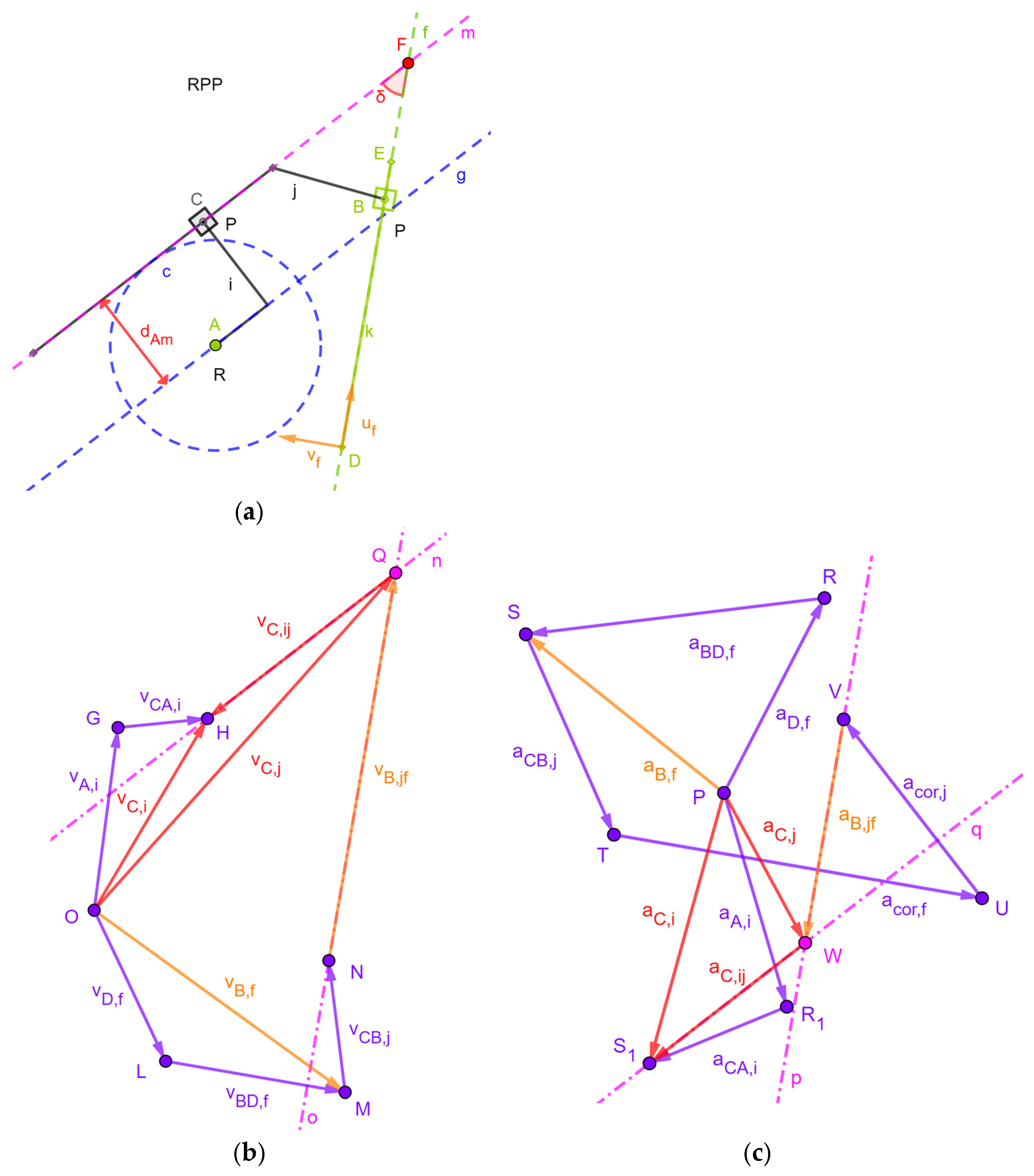
| i = Polyline(A, A − xi*um, A − xi*um − dAm*vm) | (it generates a polyline with two sides, one parallel and the other perpendicular to line m, that represents link i and xi as parameter of the object) |
| C = Intersect(i, j) | (it generate point C as the intersection between the two polylines i and j) |
| Polygon(C + 0.5*aP*(vm − um), C − 0.5*aP*(um + vm), 4) | (it generates a regular polygon centered at C and with four sides (i.e., a square), parallel to um or vm, whose length is the already-defined parameter aP) |
| O = (xO,yO) | (it generates point O and its coordinates as parameters of the object) |
| vA,i = Translate(Vector((vA,x,vA,y)),O) | (it generates the known velocity vector vA,i together with its components as parameters of the object and applies it to point O (see Figure 7b)) |
| G = O + vA,i | (it generates point G located at the point of the arrow representing vA,i) |
| ωf = Slider(ωf,min, ωf,max, Δωf) | (it generates the variable ωf (necessary to assign the angular velocity, ωf, of line f) ranging from ωf,min to ωf,max with increment Δωf) |
| ωj = ωf | (it generates the dependent variable ωj (i.e., the signed magnitude of the angular velocity of link j)) |
| ωi = ωf | (it generates the dependent variable ωi (i.e., the signed magnitude of the angular velocity of link i)) |
| vCA,i = Translate(Vector(ωi*|C − A|*UnitPerpendicularVector(Segment(A,C))),G) | (it generates the vector representing the velocity difference vCA,i and applies it to H (see Figure 7b)) |
| H = G + vCA,i | (it generates point H located at the point of the arrow representing vCA,i) |
| n = Line(H,m) | (it generates a line passing through H and parallel to line m) |
| vC,i = Vector(O,H) | (it generates a vector representing vC,I and applies it to H) |
| vD,f = Translate(Vector((vD,x,vD,y)),O) | (it generates the known velocity vector vD,f together with its components as parameters of the object and applies it to point O (see Figure 7b)) |
| L = O + vD,f | (it generates point L located at the point of the arrow representing vD,f) |
| vBD,f = Translate(Vector(ωf*|B − D|*vf),L) | (it generates the vector representing the velocity difference vBD,f and applies it to L (see Figure 7b)) |
| M = L + vBD,f | (it generates point H located at the point of the arrow representing vBD,f) |
| vB,f = Vector(O,M) | (it generates the arrow representing the velocity vB,f) |
| vCB,j = Translate(Vector(ωj*|C − B|*UnitPerpendicularVector(Segment(B,C))),M) | (it generates the vector representing the velocity difference vCB,j and applies it to M (see Figure 7b)) |
| N = M+ vCB,j | (it generates point N located at the point of the arrow representing vCB,j) |
| o = Line(N,uf) | (it generates a line passing through N and parallel to uf, that is, parallel to the relative velocity vB,jf) |
| Q = Intersect(o,n) | (it generates point Q at the intersection of lines o and n (point Q geometrically solves Equation (13))) |
| vB,jf = Vector(N,Q) | (it generates the arrow representing the relative velocity vB,jf) |
| vC,ij = Vector(Q,H) | (it generates the arrow representing the relative velocity vC,ij) |
| vC,j = Vector(O,H) | (it generates the arrow representing the sought-after velocity vC,j) |
| P = (xP,yP) | (it generates point P and its coordinates as parameters of the object) |
| αf = Slider(αf,min, αf,max, Δαf) | (it generates the variable αf (necessary to assign the angular acceleration, αf, of line f) ranging from αf,min to αf,max with increment Δαf) |
| αj = αf | (it generates the dependent variable αj (i.e., the signed magnitude of the angular acceleration of link j)) |
| αi = αf | (it generates the dependent variable αi (i.e., the signed magnitude of the angular acceleration of link i)) |
| aD,f = Translate(Vector((aD,x,aD,y)),P) | (it generates the known acceleration vector aD,f together with its components as parameters of the object and applies it to point P (see Figure 7c)) |
| R = P + aD,f | (it generates point R located at the point of the arrow representing aD,f) |
| aBD,f = Translate(Vector((αf*vf − ωf2*uf)*|B − D|),R) | (it generates the vector representing the acceleration difference aBD,f and applies it to R (see Figure 7c)) |
| S = R + aBD,f | (it generates point S located at the point of the arrow representing aBD,f) |
| aB,f = Vector(P,S) | (it generates the arrow representing the acceleration aB,f) |
| aCB,j = Translate(Vector((αj* UnitPerpendicularVector(Segment(B,C)) − ωj2*UnitVector(Segment(B,C))*|C − B|), S) | (it generates the vector representing the acceleration difference aCB,j and applies it to S (see Figure 7c)) |
| T = S + aCB,j | (it generates point T located at the point of the arrow representing aCB,j) |
| acor,f = Translate(Vector(2*ωf*Dot(vB,jf,uf)*vf),T) | (it generates the vector representing the Coriolis acceleration acor,f and applies it to T (see Figure 7c)) |
| U = T + acor,f | (it generates point U located at the point of the arrow representing acor,f) |
| acor,j = Translate(Vector(2*ωj*Dot(vC,ij,um)*vm),U) | (it generates the vector representing the Coriolis acceleration acor,j and applies it to U (see Figure 7c)) |
| V = U+ acor,j | (it generates point V located at the point of the arrow representing acor,j) |
| p = Line(V, uf) | (it generates a line passing through U and parallel to uf, that is, parallel to the relative acceleration aB,jf) |
| aA,i = Translate(Vector((aA,x,aA,y)),P) | (it generates the known acceleration vector aA,i together with its components as parameters of the object and applies it to point P (see Figure 7c)) |
| R1 = P + aA,i | (it generates point R1 located at the point of the arrow representing aA,i) |
| aCA,i = Translate(Vector((αi* UnitPerpendicularVector(Segment(A,C)) − ωj2*UnitVector(Segment(A,C))*|C − A|), R1) | (it generates the vector representing the acceleration difference aCA,i and applies it to R1 (see Figure 7c)) |
| S1 = R1+ aCA,i | (it generates point S1 located at the point of the arrow representing aCA,i) |
| aC,i = Vector(P,S1) | (it generates the arrow representing the acceleration aC,i) |
| q = Line(S1,um) | (it generates a line passing through S1 and parallel to um, that is, parallel to the relative acceleration aC,ij) |
| W = Intersect(p,q) | (it generates point W at the intersection of lines p and q (point W geometrically solves Equation (14))) |
| aB,jf = Vector(V,W) | (it generates the arrow representing the relative acceleration aB,jf) |
| aC,ij = Vector(W,S1) | (it generates the arrow representing the relative acceleration aC,ij) |
| aC,j = Vector(P,W) | (it generates the arrow representing the acceleration aC,j) |
Appendix B
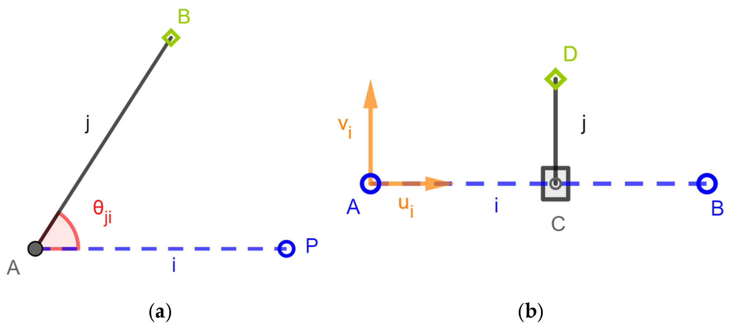
| A = (xA, yA) | (it generates point A and its coordinates as parameters of the object) |
| P = (xP, yP) | (it generates point P and its coordinates as parameters of the object) |
| i = Segment(A,P) | (it generates the segment AP representing link i) |
| r = Slider(rmin, rmax, Δr) | (it generates the linear parameter r, ranging from rmin to rmax with increments of Δr, to use for changing the length of link j) |
| θji = Slider(0, 360, 1) | (it generates the actuated joint variable θji, ranging from 0° to 360° with increment of 1° as a scalar parameter; such a command is replaceable through the analytic expression that gives θji as a function of the time, say t, after having defined t with the command “Slider()”) |
| ui = UnitVector(i) | (it generates the unit vector ui, parallel to segment i and located on it) |
| B = Rotate(A + r*ui, θji, A) | (it generates point B as the new position of point P’ = A + r*ui after the segment AP’ has rotated around point A of θji) |
| j = Segment(A, B) | (it generates the segment AB representing link j) |
| Angle(P, A, B) | (this command just makes the angle θji visible on the sketch) |
| A = (xA, yA) | (it generates point A and its coordinates as parameters of the object) |
| B = (xB, yB) | (it generates point B and its coordinates as parameters of the object) |
| i = Segment(A, B) | (it generates the segment AB representing link i) |
| d = Slider(dmin, dmax, Δd) | (it generates the linear parameter d, ranging from dmin to dmax with an increments of Δd, to use for changing the geometry of link j) |
| AC = Slider(0, abs(B − A), ΔAC) | (it generates the actuated joint variable AC as a scalar parameter, ranging from 0 to abs(B − A), which computes the length of segment AB, with an increment of ΔAC. Such a command is replaceable through the analytic expression that gives AC as a function of the time, say t, after having defined t with the command “Slider()”) |
| ui = UnitVector(i) | (it generates the unit vector ui, parallel to segment i and located on it) |
| vi = UnitPerpendicularVector(i) | (it generates the unit vector vi, perpendicular to segment i) |
| C = A + AC*ui | (it generates point C) |
| D = C + d*vi | (it generates point D) |
| j = Segment(C, D) | (it generates the segment CD representing link j) |
| Polygon(C + 0.5*aP*(vi − ui), C − 0.5*aP*(ui + vi), 4) | (it generates a regular polygon centered at C and with four sides (i.e., a square), parallel to ui or vi, whose length is aP and aP as parameter of the object) |
Appendix C
| A = (xA,yA) | (it generates point A and its coordinates as parameters of the object) |
| B = (xB,yB) | (it generates point B and its coordinates as parameters of the object) |
| f = Segment(A,B) | (it generates the segment AB representing link 1, that is, the frame) |
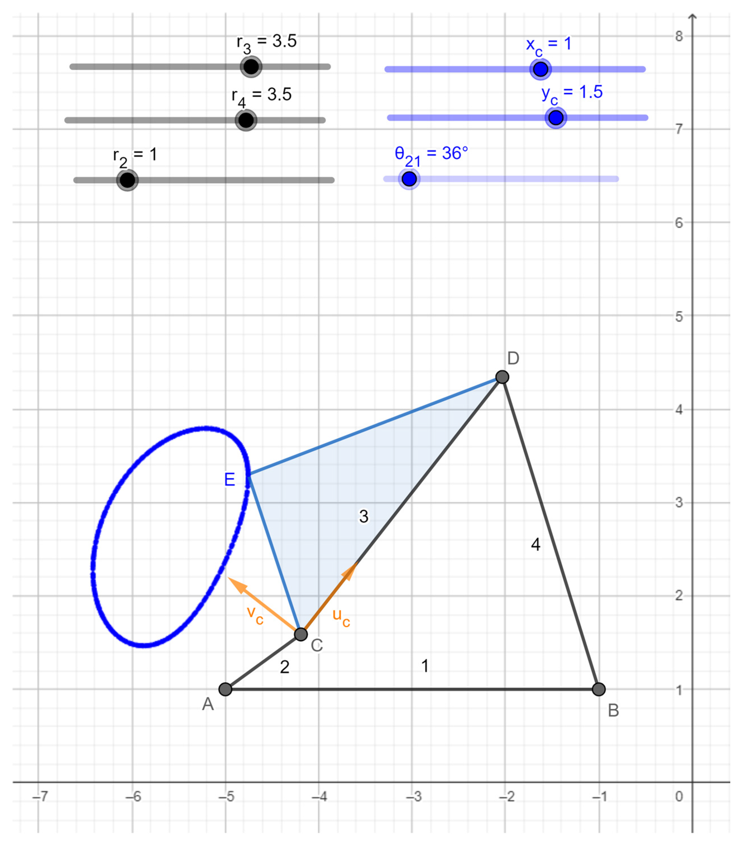
| r2 = Slider(r2,min, r2,max, Δr2) | (it generates the variable r2 (necessary to assign the crank length) ranging from r2,min to r2,max with increment Δr2) |
| θ21 = Slider(0°, 360°, 1°) | (it generates the crank angle θ21 to use for animating the sketch) |
| C = Rotate(A+ r2*UnitVector(Segment(A,B)), θ21,A) | (it generates the movable ending of the crank) |
| g = Segment(A,C) | (it generates the segment AC representing link 2, that is, the crank) |
| r3 = Slider(r3,min, r3,max, Δr3) | (it generates the variable r3 (necessary to assign the coupler length) ranging from r3,min to r3,max with increment Δr3) |
| r4 = Slider(r4,min, r4,max, Δr4) | (it generates the variable r4 (necessary to assign the rocker length) ranging from r4,min to r4,max with increment Δr4) |
| D = Intersect(Circle(C,r3), Circle(B,r4)) | (it generates the center, D, of the R-pair joining the coupler to the rocker) |
| h = Segment(C,D) | (it generates the segment CD representing link 3, that is, the coupler) |
| uc = UnitVector(h) | (it generates a unit vector uc parallel to segment CD) |
| vc = UnitPerpendicularVector(h) | (it generates a unit vector vc perpendicular to segment CD) |
| i= Segment(B,D) | (it generates the segment BD representing link 4, that is, the rocker) |
| E = C + xc*uc+ yc*vc | (it generates the tracing point, E, that draws the coupler curve and the “Slider”s of the variable parameters xc and yc necessary to change its position on the coupler) |
| Polygon(C,D,E) | (it generates the triangle CDE fixed to the coupler) |
| T = Slider(Tmin, Tmax, ΔT) | (it generates the variable T) |
| t = Slider(0, T, 0.01) | (it generates the variable t (time), necessary to give a reference time to the linkage animation, ranging from 0 s to T s with increment 0.01 s) |
| ω2 = 2*π/T | (it generates the dependent variable ω2, necessary to assign the signed magnitude of the crank angular velocity) |
| θ21 = ω2*t*180°/π | (it generates the crank angle θ21 in degrees) |
| A = (xA,yA) | (it generates point A and its coordinates as parameters of the object) |
| B = (xB,yB) | (it generates point B and its coordinates as parameters of the object) |
| f = Segment(A,B) | (it generates the segment AB representing link 1, that is, the frame) |
| a2 = Slider(a2,min, a2,max, Δa2) | (it generates the variable a2 (necessary to assign the crank length) ranging from a2,min to a2,max with increment Δa2) |
| C = Rotate(A+ a2*UnitVector(f), θ21,A) | (it generates the movable ending of the crank) |
| g = Segment(A,C) | (it generates the segment AC representing link 2, that is, the crank) |
| a3 = Slider(a3,min, a3,max, Δa3) | (it generates the variable a3 (necessary to assign the coupler length) ranging from a3,min to a3,max with increment Δa3) |
| a4 = Slider(a4,min, a4,max, Δa4) | (it generates the variable a4 (necessary to assign the rocker length) ranging from a4,min to a4,max with increment Δa4) |
| D = Intersect(Circle(C,a3), Circle(B,a4)) | (it generates the center, D, of the R-pair joining the coupler to the rocker) |
| h = Segment(C,D) | (it generates the segment CD representing link 3, that is, the coupler) |
| i = Segment(D,B) | (it generates the segment BD representing link 4, that is, the rocker) |
| E2 = A + x2*UnitVector(g)+ y2*UnitPerpendicularVector(g) | (it generates point E2 fixed to the crank and the associated variable parameters x2 and y2) |
| t2 = Polygon(A,C,E2) | (it generates a triangular shape of the crank) |
| A2 = Area(t2) | (it computes the area of t2) |
| G2 = Centroid(t2) | (it generates point G2 located at the centroid of t2) |
| I2 = (1/36)*(a2*y23 + y2*a23 − y2*x2*a22 + a2*y2*x22) | (it computes the area moment of inertia of t2 with respect to its centroid) |
| E3 = C + x3*UnitVector(h)+ y3*UnitPerpendicularVector(h) | (it generates point E3 fixed to the coupler and the associated variable parameters x3 and y3) |
| t3 = Polygon(C,D,E3) | (it generates the triangular shape of the coupler) |
| A3 = Area(t3) | (it computes the area of t3) |
| G3 = Centroid(t3) | (it generates point G3 located at the centroid of t3) |
| I3 = (1/36)*(a3*y33 + y3*a33 − y3*x3*a32 + a3*y3*x32) | (it computes the area moment of inertia of t3 with respect to its centroid) |
| E4 = D + x4*UnitVector(i)+ y4*UnitPerpendicularVector(i) | (it generates point E4 fixed to the rocker and the associated variable parameters x4 and y4) |
| t4 = Polygon(D,B,E4) | (it generates the triangular shape of the rocker) |
| A4 = Area(t4) | (it computes the area of t4) |
| G4 = Centroid(t4) | (it generates point G4 located at the centroid of t4) |
| I4 = (1/36)*(a4*y43 + y4*a43 − y4*x4*a42 + a4*y4*x42) | (it computes the area moment of inertia of t4 with respect to its centroid) |
| O = (xO,yO) | (it generates point O and its coordinates as parameters of the object) |
| u2 = UnitVector(Segment(A,C)) | (it generates a unit vector with the same direction as vector (C − A)) |
| v2 = UnitPerpendicularVector(Segment(A,C)) | (it generates a unit vector with the same direction as vector k × (C − A)) |
| u3 = UnitVector(Segment(C,D)) | (it generates a unit vector with the same direction as vector (D − C)) |
| v3 = UnitPerpendicularVector(Segment(C,D)) | (it generates a unit vector with the same direction as vector k × (D − C)) |
| u4 = UnitVector(Segment(B,D)) | (it generates a unit vector with the same direction as vector (D − B)) |
| v4 = UnitPerpendicularVector(Segment(B,D)) | (it generates a unit vector with the same direction as vector k × (D − B)) |
| vC,2 = Translate(Vector(ω2*|C − A|*v2),O) | (it generates the arrow representing the velocity vC,2 and applies it at point O) |
| E = O+ vC,2 | (it generates point E located at the point of the arrow representing vC,2) |
| F = Intersect(Line(E,v3),Line(O,v4)) | (it generates point F, which geometrically solves the velocity loop equation) |
| vD,3 = Vector(O,F) | (it generates the arrow representing the velocity vD,3) |
| vDC,3 = Vector(E,F) | (it generates the arrow representing the velocity vDC,3) |
| ω3 = Dot(vDC,3, v3)/|D − C| | (it computes the signed magnitude, ω3, of link-3′ s angular velocity) |
| ω4 = Dot(vD,3, v4)/|D − B| | (it computes the signed magnitude, ω4, of link-4′ s angular velocity) |
| P = (xP,yP) | (it generates point P and its coordinates as parameters of the object) |
| α2 = Slider(α2,min, α2,max,Δα2) | (it generates the variable α2, necessary to assign the signed magnitude of crank’s angular acceleration, ranging from α2,min to α2,max with increment Δα2) |
| aC,2 = Translate(Vector((α2*v2 − ω22*u2)*|C − A|),P) | (it generates the vector representing the acceleration aC,2 and applies it to P) |
| G = P + aC,2 | (it generates point G located at the point of the arrow representing aC,2) |
| aDB‖,4 = Translate(Vector(−ω42*(D − B)),P) | (it generates the vector representing the component aDB‖,4 of acceleration difference and applies it to P) |
| H = P+ aDB‖,4 | (it generates point H located at the point of the arrow representing aDB‖,4) |
| aDC‖,3 = Translate(Vector(−ω32*(D − C)),G) | (it generates the vector representing the component aDC‖,3 of acceleration difference and applies it to G) |
| L = G + aDC‖,3 | (it generates point L located at the point of the arrow representing aDC‖,3) |
| M = Intersect(Line(H,v4),Line(L,v3)) | (it generates point M, which geometrically solves the acceleration loop equation) |
| aDC⊥,3 = Vector(L,M) | (it generates the vector representing aDC⊥,3) |
| aDB⊥,4 = Vector(H,M) | (it generates the vector representing aDB⊥,4) |
| aD,4 = Vector(P,M) | (it generates the vector representing aD,4) |
| aDC,3 = Vector(G,M) | (it generates the vector representing aDC,3) |
| α3 = Dot(aDC⊥,3, v3)/|D − C| | (it computes the signed magnitude, α3, of link-3′ s angular acceleration) |
| α4 = Dot(aDB⊥,4, v4)/|D − B| | (it computes the signed magnitude, α4, of link-4′ s angular acceleration) |
| P’ = (xP’,yP’) | (it generates point P’ and its coordinates as parameters of the object) |
| aC,3 = Translate(aC,2,P’) | (it applies at P’ a vector equal to aC,2 (=aC,3)) |
| G’ = P’+ aC,3 | (it generates point G located at the point of the arrow representing aC,3) |
| aD,3 = Translate(aD,2,P’) | (it applies at P’ a vector equal to aD,4 (=aD,3)) |
| M’ = P’+ aD,3 | (it generates point M’ located at the point of the arrow representing aD,3) |
| aDC,3′ = Vector(G’,M’) | (it applies at G’ a vector equal to aDC,3) |
| m = Rotate(Segment(P’,G’), Angle(C,A,G2),P’) | with one ending at P’) |
| n = Rotate(Segment(P’,G’), Angle(A,C,G2),G’) | with one ending at G’) |
| G2′ = Intersect(m,n) | ) |
| aG2 = Vector(P’,G2′) | ) |
| p = Rotate(Segment(G’,M’), Angle(D,C,G3),G’) | with one ending at G’) |
| q = Rotate(Segment(G’,M’), Angle(C,D,G3),M’) | with one ending at M’) |
| G3′ = Intersect(p,q) | ) |
| aG3 = Vector(P’,G3′) | ) |
| r = Rotate(Segment(P’,M’), Angle(D,B,G4),P’) | with one ending at P’) |
| s = Rotate(Segment(P’,M’), Angle(B,D,G4),M’) | with one ending at M’) |
| G4′ = Intersect(r,s) | ) |
| aG4 = Vector(P’,G4′) | ) |
| ρ = Slider(ρmin, ρmax,Δ ρ) | (it generates the variable ρ, necessary to assign the areal density of the links, ranging from ρmin to ρmax with increment Δρ) |
| m2 = ρA2 | (it computes the mass of link 2) |
| J2 = ρI2 | (it computes the mass moment of inertia about the barycenter of link 2) |
| m3 = ρA3 | (it computes the mass of link 3) |
| J3 = ρI3 | (it computes the mass moment of inertia about the barycenter of link 3) |
| m4 = ρA4 | (it computes the mass of link 4) |
| J4 = ρI4 | (it computes the mass moment of inertia about the barycenter of link 4) |
| Q4 = −m4*aG4 | (it computes the resultant of the inertia forces of link 4) |
| vF4 = UnitPerpendicularVector(Q4) | (it generates a unit vector perpendicular to Q4) |
| P4 = G4 + vF4*(J4*α4/abs(Q4)) | (it generates a point of the central axis of the inertia forces applied to link 4) |
| F4 = Translate(Q4,P4) | (it applies Q4 at P4) |
| a = Line(C,D) | (it generates the line of action of F34,4) |
| K4 = Intersect(a,Line(P4,F4)) | (it generate the intersection of the lines of action of F4 and F34,4) |
| e = Segment(P4,K4) | (it generates a segment lying on the action line of F4) |
| f1 = Segment(B,K4) | (it generates a segment lying on the action line of F14,4) |
| R4 = P4 + F4 | (it generates a point located at point of the arrow representing F4) |
| N4 = Intersect(Line(P4,f1), Line(R4,a)) | (it generates point N4 that graphically solves the force equilibrium equation F4 + F14,4 + F34,4 = 0) |
| F34,4 = Vector(R4,N4) | (it generates a vector representing force F34,4) |
| F14,4 = Vector(N4,P4) | (it generates a vector representing force F14,4) |
| F34,4′ = Translate(F34,4,D) | (it applies force F34,4 on its line of action) |
| F14,4′ = Translate(F14,4,B) | (it applies force F14,4 on its line of action) |
| F32,4 = Translate(−F34,4,C) | (it applies force F32,4 on its line of action) |
| F12,4 = Translate(−F32,4,A) | (it applies force F12,4 on its line of action) |
| Q3 = −m3*aG3 | (it computes the resultant of the inertia forces of link 3) |
| vF3 = UnitPerpendicularVector(Q3) | (it generates a unit vector perpendicular to Q3) |
| P3 = G3 + vF3*(J3*α3/abs(Q3)) | (it generates a point of the central axis of the inertia forces applied to link 3) |
| F3 = Translate(Q3,P3) | (it applies Q3 at P3) |
| g1 = Line(B,D) | (it generates the line of action of F34,3) |
| K3 = Intersect(g1,Line(P3,F3)) | (it generate the intersection of the lines of action of F3 and F34,3) |
| h1 = Segment(C,K3) | (it generates a segment lying on the action line of F23,3) |
| h2 = Segment(P3,K3) | (it generates a segment lying on the action line of F3) |
| R3 = P3 + F3 | (it generates a point located at point of the arrow representing F3) |
| N3 = Intersect(Line(P3,g1), Line(R3,h1)) | (it generates point N3 that graphically solves the force equilibrium equation F3 + F23,3 + F43,3 = 0) |
| F23,3 = Vector(R4,N3) | (it generates a vector representing force F23,3) |
| F43,3 = Vector(N3,P3) | (it generates a vector representing force F43,3) |
| F34,3 = Translate(−F43,3,D) | (it applies force F43,3 on its line of action) |
| F32,3 = Translate(−F23,3,C) | (it applies force F23,3 on its line of action) |
| F14,3 = Translate(−F34,3,B) | (it applies force F14,3 on its line of action) |
| F12,3 = Translate(−F32,3,A) | (it applies force F12,3 on its line of action) |
| Q2 = −m2*aG2 | (it computes the resultant of the inertia forces of link 2) |
| vF2 = UnitPerpendicularVector(Q2) | (it generates a unit vector perpendicular to Q2) |
| P2 = G2 + vF2*(J2*α2/abs(Q2)) | (it generates a point of the central axis of the inertia forces applied to link 2) |
| F2 = Translate(Q2,P2) | (it applies Q2 at P2) |
| F12,2 = Translate(−F2,A) | (it applies force F12,2 on its line of action) |
| F14 = Translate(F14,4 + F14,3,B) | (it applies the resultant F14 on its line of action) |
| F34 = Translate(F34,4 + F34,3,D) | (it applies the resultant F34 on its line of action) |
| F12 = Translate(F12,4 + F12,3 + F12,2,A) | (it applies the resultant F12 on its line of action) |
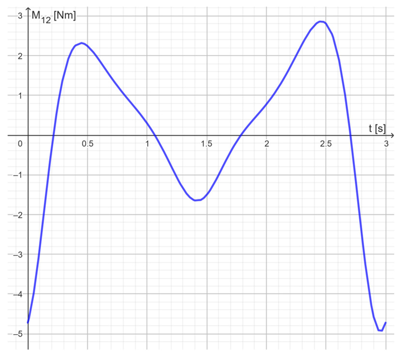
| M12 = −(x(P2) − x(A))*y(F2) + (y(P2) − y(A))*x(F2) − (x(C) − x(A))*y(F32) + (y(C) − y(A))*x(F32) | (it computes the generalized torque the actuator must apply) |
| T = Slider(Tmin, Tmax, ΔT) | (it generates the variable T) |
| t = Slider(0, T, 0.01) | (it generates the variable t (time), necessary to give a reference time to the linkage animation, ranging from 0 s to T s with increment 0.01 s) |
| ω2 = 2*π/T | (it generates the dependent variable ω2, necessary to assign the signed magnitude of the crank angular velocity) |
| θ21 = ω2*t*180°/π | (it generates the crank angle θ21 in degrees) |
| A = (xA,yA) | (it generates point A and its coordinates as parameters of the object) |
| B = A+(0, − a1) | (it generates point B and the “Slider” of frame geometry’s parameter a1) |
| f = Segment(A,B) | (it generates the segment AB representing the first part of link 1, which is the frame) |
| a2 = Slider(a2,min, a2,max, Δa2) | (it generates the variable a2 (necessary to assign the crank length) ranging from a2,min to a2,max with increment Δa2) |
| u1 = UnitVector(Segment(A,Rotate(B,90°,A))) | (it generates unit vector u1) |
| v1 = UnitPerpendicularVector(u1) | (it generates a unit vector perpendicular to u1) |
| C = Rotate(A+ a2*u1, θ21,A) | (it generates the movable ending of the crank) |
| g = Segment(A,C) | (it generates the segment AC representing link 2, that is, the crank) |
| a4 = Slider(a4,min, a4,max, Δa4) | (it generates the variable a4 (necessary to assign the length of segment BD representing link 4) ranging from a4,min to a4,max with increment Δa4) |
| D = B+a4*UnitVector(Segment(B,C)) | (it generates point D, which is the center of the R-pair joining links 4 and 5) |
| h = Segment(B,D) | (it generates the segment BD representing link 4) |
| Polygon(C + 0.5*aP*(UnitPerpendicularVector(h) − UnitVector(h)),C − 0.5*aP*(UnitVector(h) + UnitPerpendicularVector(h)),4) | (it generates a square centered at C with two sides parallel to segment BD and the associated variable aP, which plays the role of side length) |
| BB = B+(a1 + b1)*v1 | (it generates point BB lying on the horizontal dash-dot line of Figure 12 and the associated frame geometry parameter b1) |
| i = Segment(BB − (a6 − 2)*u1, BB + (a6 + 2)*u1) | (it generates the dash–dot segment of Figure 12, which plays the role of joint axis, and the associated parameter a6, which assigns its half-length) |
| E = Intersect(Circle(D,a5),Line(BB,u1)) | (it generates point E and the parameter a5 that is the length of segment DE) |
| j = Segment(D,E) | (it generates the segment DE representing link 5) |
| Polygon(E + 0.5*aP*(v1 − u1),E − 0.5*aP*(u1+ v1),4) | (it generates a square centered at E with two horizontal sides) |
| i’ = Translate(i,Vector(−(0.5 aP + 0.01)*v1)) | (it generates the black horizontal line of Figure 12, which is the second part of link 1 (the frame)) |
| O = (xO,yO) | (it generates point O and its coordinates as parameters of the object) |
| vC,2 = Translate(ω2*PerpendicularVector(Segment(A,C)),O) | (it generates the vector representing velocity vC,2 and applies it at point O) |
| F = O+ vC,2 | (it generates point F at the point of the arrow representing vC,2) |
| G = Intersect(Line(O,Vector(UnitPerpendicularVector(h))),Line(F,Vector(UnitVector(h)))) | ) |
| vC,4 = Vector(O,G) | (it generates the vector representing velocity vC,4) |
| vC,34 = Vector(G,F) | (it generates the vector representing relative velocity vC,34) |
| vD,4 = Translate(Vector(vC,4*abs(D − B)/abs(C − B)),O) | (it generates the vector representing velocity vD,4 (=vD,5) and applies it at point O) |
| H = O+vD,4 | (it generates point H at the point of the arrow representing vD,4 (=vD,5)) |
| L = Intersect(Line(O,i),Line(H,Vector(PerpendicularVector(Segment(D,E))))) | ) |
| vE,5 = Vector(O,L) | (it generates the vector representing velocity vE,5 (=vE,6)) |
| vED,5 = Vector(H,L) | (it generates the vector representing velocity vED,5) |
| ω4 = Dot(vC,4, UnitPerpendicularVector(Segment(B,C)))/abs(C − B) | (it computes the signed magnitude, ω4, of the angular velocity of link 4) |
| ω3 = ω4 | (it computes the signed magnitude, ω3, of the angular velocity of link 3) |
| ω5 = Dot(vED,5, UnitPerpendicularVector(Segment(D,E)))/abs(E − D) | (it computes the signed magnitude, ω5, of the angular velocity of link 5) |
| a’cor = 2*ω4*UnitPerpendicularVector(vC,34) | (it computes the Coriolis acceleration) |
| P = (xP,yP) | (it generates point P and its coordinates as parameters of the object) |
| α2 = Slider(α2,min, α2,max,Δα2) | (it generates the variable α2, necessary to assign the signed magnitude of crank’s angular acceleration, ranging from α2,min to α2,max with increment Δα2) |
| aC,2 = Translate(α2*PerpendicularVector(Vector(A,C)) − ω22*Vector(A,C),P) | (it generates the vector representing the acceleration aC,2 (=aC,3) and applies it to P) |
| M = P+aC,2 | (it generates point M located at the point of the arrow representing aC,2) |
| acor = Translate(a’cor,P) | (it generates the arrow representing Coriolis acceleration acor and applies it at P) |
| N = P+acor | (it generates point N located at the point of the arrow representing acor) |
| aC‖,4 = Translate(Vector(−ω42*(C − B)),N) | (it generates the vector representing the component aCA‖,4 (=aC‖,4) of acceleration difference aCA,4 and applies it to N) |
| Q = N+aC‖,4 | (it generates point Q located at the point of the arrow representing aC‖,4) |
| R = Intersect(Line(Q,Vector(PerpendicularVector(aC‖,4))),Line(M,Segment(B,D))) | ) |
| aC⊥,4 = Vector(Q,R) | (it generates the vector representing aCA⊥,4 (=aC⊥,4)) |
| aC,34 = Vector(R,M) | (it generates the vector representing the relative acceleration aC,34) |
| aC,4 = Vector(N,R) | (it generates the vector representing aC,4 (=aCA,4)) |
| aD,4 = Translate(Vector(aC,4*abs(D − B)/abs(C − B)),N) | (it generates the vector representing acceleration aD,4 (=aD,5) and applies it at point N) |
| S = N+aD,4 | (it generates point S located at the point of the arrow representing aD,4) |
| aED‖,5 = Translate(Vector(−ω52*(E − D)),S) | (it generates the vector representing the component aED‖,5 of acceleration difference and applies it to S) |
| U = S+ aED‖,5 | (it generates point U located at the point of the arrow representing aED‖,5) |
| V = Intersect(Line(U,Vector(PerpendicularVector(Segment(D,E)))),Line(N,u1)) | ) |
| aED⊥,5 = Vector(U,V) | (it generates the vector representing aED⊥,5) |
| aED,5 = Vector(S,V) | (it generates the vector representing aED,5) |
| aE,5 = Vector(N,V) | (it generates the vector representing aE,5 (=aE,6)) |
| α4 = Dot(aC⊥,4, UnitPerpendicularVector(Segment(B,C)))/|C − B| | (it computes the signed magnitude, α4, of link-4′ s angular acceleration) |
| α3 = α4 | (it computes the signed magnitude, α3, of link-3′ s angular acceleration) |
| α5 = Dot(aED⊥,5, UnitPerpendicularVector(Segment(D,E)))/|E − D| | (it computes the signed magnitude, α5, of link-5′ s angular acceleration) |
References
- Mirth, J.A. Parametric Modeling—A New Paradigm for Mechanisms Education? In Proceedings of the ASME 2012 International Design Engineering Technical Conferences & Computers and Information in Engineering Conference (IDETC/CIE 2012), Chicago, IL, USA, 12–15 August 2012. Paper No.: DETC2012-70175. [Google Scholar]
- Waldron, K.J.; Kinzel, G.L.; Agrawal, S.K. Kinematics, Dynamics, and Design of Machinery, 3rd ed.; John Wiley & Sons Inc.: Chichester, UK, 2016. [Google Scholar]
- Erdman, A.G. Computer-Aided Mechanism Design: Now and the Future. J. Mech. Des. 1995, 117, 93–100. [Google Scholar] [CrossRef]
- Kinzel, E.C.; Schmiedeler, J.P.; Pennock, G.R. Kinematic Synthesis for Finitely Separated Positions Using Geometric Constraint Programming. J. Mech. Des. 2006, 128, 1070–1079. [Google Scholar] [CrossRef]
- Kinzel, E.C.; Schmiedeler, J.P.; Pennock, G.R. Function Generation with Finitely Separated Precision Points Using Geometric Constraint Programming. J. Mech. Des. 2007, 129, 1185–1190. [Google Scholar] [CrossRef]
- Mirth, J.A. The Application of Geometric Constraint Programming to the Design of Motion Generating Six-Bar Linkages. In Proceedings of the ASME 2012 International Design Engineering Technical Conferences and Computers and Information in Engineering Conference, Chicago, IL, USA, 12–15 August 2012; Volume 4: 36th Mechanisms and Robotics Conference, Parts A and B. pp. 1503–1511. [Google Scholar] [CrossRef]
- Mirth, J.A. A GCP Design Approach for Infinitesimally and Multiply Separated Positions Based on the Use of Velocity and Acceleration Vector Diagrams. In Proceedings of the ASME 2014 International Design Engineering Technical Conferences and Computers and Information in Engineering Conference, Buffalo, NY, USA, 17–20 August 2014; Volume 5B. [Google Scholar] [CrossRef]
- Schmiedeler, J.P.; Clark, B.C.; Kinzel, E.C.; Pennock, G.R. Kinematic Synthesis for Infinitesimally and Multiply Separated Positions Using Geometric Constraint Programming. J. Mech. Des. 2014, 136, 034503. [Google Scholar] [CrossRef]
- Mirth, J.A. Mixed Exact and Approximate Position Design of Planar Linkages via Geometric Constraint Programming (GCP) Techniques. In Proceedings of the ASME 2015 International Design Engineering Technical Conferences and Computers and Information in Engineering Conference, Boston, MA, USA, 2–5 August 2015; Volume 5B. [Google Scholar] [CrossRef]
- Mirth, J.A. The Application of Geometric Constraint Programming to the Design of Stephenson III Dwell Linkages. In Proceedings of the ASME 2016 International Design Engineering Technical Conferences and Computers and Information in Engineering Conference, Charlotte, NC, USA, 21–24 August 2016; Volume 5B. [Google Scholar] [CrossRef]
- Zimmerman, R.A., II. Planar Linkage Synthesis for Mixed Motion, Path, and Function Generation Using Poles and Rotation Angles. J. Mechanisms Robotics 2018, 10, 025004. [Google Scholar] [CrossRef]
- Alfattani, R.; Lusk, C. Shape-Morphing Using Bistable Triangles with Dwell-Enhanced Stability. J. Mechanisms Robotics 2020, 12, 051003. [Google Scholar] [CrossRef]
- Tong, Y.; Myszka, D.H.; Murray, A.P. Four-Bar Linkage Synthesis for a Combination of Motion and Path-Point Generation. In Proceedings of the ASME 2013 International Design Engineering Technical Conferences and Computers and Information in Engineering Conference, Portland, OR, USA, 4–7 August 2013; Volume 6A. [Google Scholar] [CrossRef]
- Ting, K.; Chan, C.L. Reversible Geometric Constraint Programming on Kinematic Analysis and Synthesis of Planar Linkages. In Proceedings of the ASME 2022 International Mechanical Engineering Congress and Exposition, Columbus, OH, USA, 30 October–3 November 2022; Volume 4. [Google Scholar] [CrossRef]
- Zimmerman, R.A., II. Planar Linkage Synthesis: A Modern CAD Based Approach; Zimmerman Publishing: Novi, MI, USA, 2023; ISBN 979-8218173586. [Google Scholar]
- Simionescu, P.A. Computer-Aided Graphing and Simulation Tools for AutoCAD Users; CRC Press: New York, NY, USA, 2015; ISBN 978-1-4822-5292-7. [Google Scholar]
- Söylemez, E. Kinematic Synthesis of Mechanisms: Using Excel and GeoGebra; Springer: Cham, Switzerland, 2023; ISBN 978-3-031-30955-7. [Google Scholar]
- Venema, G.A. Exploring Advanced Euclidean Geometry with GeoGebra; Mathematical Association of America, Inc.: Washington, DC, USA, 2013; ISBN 978-1-61444-111-3. [Google Scholar]
- Assur, L.V. Research of a planar linkages with lower pairs on the basis of their structure and classification. Part 1. Bull. Petrograd Polytech. Inst. 1913, 20, 329–386. (In Russian) [Google Scholar]
- Assur, L.V. Research of a planar linkages with lower pairs on the basis of their structure and classification. Part 2. Bull. Petrograd Polytech. Inst. 1914, 21, 187–283. (In Russian) [Google Scholar]
- Assur, L.V. Investigation of Plane, Hinged Mechanisms with Lower Pairs, from the Point of View of Their Structure and Classification; Artobolevskii, I.I., Ed.; Academy of Sciences: Moscow, Russia, 1952. [Google Scholar]
- Baranov, G.G. Curso de la Teoria de Mecanismos y Maquinas; Editorial Mir: Moscow, Russia, 1979. [Google Scholar]
- Galletti, C.U. On the Position Analysis of Assur’s Groups of High Class. Meccanica 1979, 14, 6–10. [Google Scholar] [CrossRef]
- Galleti, C.U. A Note on Modular Approaches to Planar Linkage Kinematic Analysis. Mech. Mach. Theory 1986, 21, 385–391. [Google Scholar] [CrossRef]
- Rojas, N.; Thomas, F. On closed-form solutions to the position analysis of Baranov trusses. Mech. Mach. Theory 2012, 50, 179–196. [Google Scholar] [CrossRef]
- Hahn, E.; Shai, O. The Unique Engineering Properties of Assur Groups/Graphs, Assur Kinematic Chains, Baranov Trusses and Parallel Robots. In Proceedings of the ASME 2016 International Design Engineering Technical Conferences and Computers and Information in Engineering Conference (IDETC/CIE 2016), Charlotte, NC, USA, 21–24 August 2016. DETC2016-59135. [Google Scholar]
- Sun, Y.; Ge, W.; Zheng, J.; Dong, D. Solving the Kinematics of the Planar Mechanism Using Data Structures of Assur Groups. J. Mech. Robot. 2016, 8, 061002. [Google Scholar] [CrossRef]
- Huang, P.; Ding, H. Structural Synthesis of Baranov Trusses with Up to 13 Links. J. Mech. Des. 2019, 141, 072301. [Google Scholar] [CrossRef]
- Uicker, J.J., Jr.; Pennock, G.R.; Shigley, J.E. Theory of Machines and Mechanisms, 6th ed.; Cambridge University Press: Cambridge, UK, 2023; ISBN 9781009303644. [Google Scholar]
- Di Gregorio, R. A geometric and analytic technique for studying single-DOF planar mechanisms’ dynamics. Mech. Mach. Theory 2021, 168, 104609. [Google Scholar] [CrossRef]
- Di Gregorio, R. A geometric and analytic technique for studying multi-DOF planar mechanisms’ dynamics. Mech. Mach. Theory 2022, 176, 104975. [Google Scholar] [CrossRef]
- Di Gregorio, R. The Role of Instant Centers in Kinematics and Dynamics of Planar Mechanisms: Review of LaMaViP’s Contributions. Machines 2022, 10, 732. [Google Scholar] [CrossRef]


Disclaimer/Publisher’s Note: The statements, opinions and data contained in all publications are solely those of the individual author(s) and contributor(s) and not of MDPI and/or the editor(s). MDPI and/or the editor(s) disclaim responsibility for any injury to people or property resulting from any ideas, methods, instructions or products referred to in the content. |
© 2024 by the authors. Licensee MDPI, Basel, Switzerland. This article is an open access article distributed under the terms and conditions of the Creative Commons Attribution (CC BY) license (https://creativecommons.org/licenses/by/4.0/).
Share and Cite
Di Gregorio, R.; Cinti, T. Geometric Constraint Programming (GCP) Implemented Through GeoGebra to Study/Design Planar Linkages. Machines 2024, 12, 825. https://doi.org/10.3390/machines12110825
Di Gregorio R, Cinti T. Geometric Constraint Programming (GCP) Implemented Through GeoGebra to Study/Design Planar Linkages. Machines. 2024; 12(11):825. https://doi.org/10.3390/machines12110825
Chicago/Turabian StyleDi Gregorio, Raffaele, and Tommaso Cinti. 2024. "Geometric Constraint Programming (GCP) Implemented Through GeoGebra to Study/Design Planar Linkages" Machines 12, no. 11: 825. https://doi.org/10.3390/machines12110825
APA StyleDi Gregorio, R., & Cinti, T. (2024). Geometric Constraint Programming (GCP) Implemented Through GeoGebra to Study/Design Planar Linkages. Machines, 12(11), 825. https://doi.org/10.3390/machines12110825