1. Introduction
Rotating machinery is widely used in modern industrial, civil, and military fields. Due to its complex working environment, failures may occur, which will incur increased operation and maintenance costs and the loss of productivity [
1]. Sometimes it may even lead to catastrophic accidents. Therefore, fault diagnosis and condition monitoring is one of the research foci in rotating machinery [
2]. Nowadays, damage detection and condition monitoring based on vibration analysis is still the most commonly used method [
3,
4].
Synchronous analysis is an effective component of rotating machinery vibration signal processing. Usually, in order to diagnose faults of rotating machinery, it is necessary to extract the relevant fault features from the vibration response through signal processing techniques [
5]. These fault features are commonly associated with the shaft rotation speed. Hence, if the shaft rotating speed varies, the damage features may diminish or even vanish on spectrum due to the smearing effect. Synchronous analysis is a technique developed by integrating shaft speed into vibration signal processing, namely, synchronous resampling. In the synchronous resampling technique, the signal is not discretized in forms of equal time intervals, but in forms of equal shaft rotation angles. Thus, the shaft rotation effect is significantly reduced or eliminated, and the smearing effect caused by variations in shaft speed is reduced or eliminated.
Techniques related to synchronous analysis have demonstrated their effectiveness and practicality in rotation machinery damage detection and condition monitoring [
6,
7,
8], especially in cases with variable speed operations. For example, synchronous averaging can effectively separate the information synchronized with the shaft speed [
9,
10,
11,
12], such as the shaft speed response, the gear meshing response, and their high-order harmonics. For bearing fault analysis, the application of the virtual shaft concept [
13] has been introduced with success. In the technique, a virtual shaft is introduced into signal processing, so that the bearing damage feature is synchronized with the virtual shaft. Thus, the effective synchronous averaging technique can then be performed in the virtual shaft domain, to improve the bearing damage signature signal-to-noise ratio (SNR) [
14]. Synchronous analysis is also frequently integrated with other bearing fault diagnosis methods, like the popular acceleration enveloping analysis (AEA) [
15], and spectral kurtosis analysis [
16,
17]. The AEA method uses a band-pass or high-pass filter to separate the dynamic responses induced by damage. Spectral kurtosis analysis can improve the band-pass filter design by figuring out an optimal frequency range through kurtogram analysis. These techniques will be utilized as a reference baseline in our research as well. More details regarding the utilizing of synchronous analysis technologies for bearing fault diagnosis can be found in the open literature, such as references [
18,
19].
The prerequisite for synchronous analysis is synchronous sampling. Modern analog-to-digital conversion (ADC) is usually achieved by digitizing an analog signal to an equal time interval data series [
20]. The resulting digital series has an equal time interval, and the time interval is specified by the sampling rate. In the case of constant speed operations, equal delta time data acquisition is equivalent to the equal shaft rotation angle data acquisition. Nevertheless, the sampling is not necessarily the integer multiple of the shaft speed, and therefore a full-cycle sampling within a shaft cycle may not be guaranteed. As a result, in the spectrum, the shaft-related feature frequency may have energy leakage, although it has eliminated the smearing effect. In general, energy leakage can be minimized or even eliminated by increasing the sampling rate [
21]. For variable speed operations, however, if the equal delta time interval data series is directly converted into frequency domain, the shaft-related features will have the inevitable smearing phenomenon. To avoid it, a synchronization sampling is required.
The conventional synchronization sampling method relies on hardware devices to generate an equidistant sampling clock. This clock is subsequently employed to regulate the data acquisition process. Since such a sampling clock is determined by hardware, the sampling precision and resolution is limited. With the development of computer hardware and software technologies, synchronous resampling is currently achieved by reprocessing the equal delta time interval data series in the digital domain [
22]. At present, synchronous acquisition methods based on digital processing can be categorized into two groups. One is the hybrid synchronous analysis method, which uses a piece of hardware to record the shaft rotation pulse train. The recorded speed signal is then used to assist the synchronous resampling through a designed software [
23,
24,
25]. This process is known as computed order tracking (COT). The other group is based on the instantaneous frequency estimation from the vibration response, without a tachometer or a key-phasor installed on the shaft [
26,
27].
For a given function of time, mathematically, the synchronous resampling process is used to find the independent variable values for given dependent variable values. Usually, this is an iteration process, and therefore it consumes a considerable amount of CPU time. In advanced rotating machinery tests, such as the high-speed railway bench test [
28,
29], it takes a long time for the machine to experience many different operational modes during the testing procedure. Any uneconomical processing steps may prevent the application of the process to the entire time range. On the other hand, in quasi real-time analysis, it is always beneficial to minimize the processing time in each and every time step [
30]. Therefore, it is important to further reduce the processing time while maintaining high accuracy in data resampling for synchronous analysis.
Towards improving the efficiency and accuracy of synchronous signal processing, this paper presents a fast yet accurate synchronization time-point calculation method based on the inverse function interpolation. This approach achieves the computation of timestamps corresponding to the equal rotation angles of the shaft through a process of evaluating dependent variables for given independent variables. Notably, this method avoids an iterative process, resulting in a significant reduction in computational time costs. Analysis of the numerical simulations and real examples demonstrated the feasibility, effectiveness, and practicality of the proposed approach.
The rest of this paper is structured as follows:
Section 2 details the synchronous resampling method based on inverse function interpolation.
Section 3 verifies the feasibility and advantages of this methodology through numerical simulation.
Section 4 verifies the proposed methodology with two practical cases of railway bearing damage detection. Finally,
Section 5 provides the conclusion.
2. Synchronous Resampling Method Based on Inverse Function Interpolation
2.1. Basic Principles of Synchronous Resampling
Modern synchronous resampling is mostly carried out in the digital domain, as shown in
Figure 1. The vibration response signal and key-phasor signal are obtained from a rotating machine through sensors. They are then discretized by a high-frequency and high-resolution ADC with an equal delta time interval simultaneously. For the convenience of explanation, the vibration response signal is represented by the shaft fundamental response only. A key-phasor signal is a signal correlated with the rotational phase of a mechanical shaft in a rotating system. The key-phasor signal is usually measured by a proximity probe with respect to the key on the shaft, and then converted to the format of transistor–transistor logic (TTL) pulses. The pulses are generated at a rate of one pulse per shaft rotation cycle. Then, from the digitized key-phasor signal, the shaft speed 1/rev time mark and the synchronous timestamps for the equal delta shaft angle are determined numerically. In cases where the shaft speed remains constant, synchronous timestamps are uniformly distributed along the time axis. Conversely, for a variable-speed case, these synchronous timestamps will be uneven on the time axis and need to be evaluated accordingly. Following synchronous timestamps, the synchronous vibration response can be obtained through a numerical processing scheme such as interpolation.
Digital-domain synchronous resampling consists of three major steps. The first step is to determine the time mark of every full-cycle shaft rotation from the digitized key-phasor signal. The second step is to discern the timestamps corresponding to each equal delta shaft angle point. The last step is to utilize the calculated timestamps to resample the equal delta-time digitized signal to obtain the synchronous response data series.
In general, the first step can be obtained by identifying the trigger position of the shaft key-phasor pulse train, or the shaft whole-revolution time location from the shaft instantaneous speed. While the third step can be achieved by a general one-dimensional interpolation algorithm (such as the interp1 function in MATLAB). The second step is more involved, especially if the shaft speed changes substantially.
As shown in
Figure 2a, assuming that
and
are the time marks of two consecutive key-phasor pulses (or shaft whole-revolution time marks), the corresponding shaft speeds at
and
are
and
, respectively. The unit of shaft speed in this paper is revolution per second,
. For a variable speed operation,
≠
. According to the definition of a complete shaft rotation, we have
In the most general case, assuming the number of synchronous resampling points is
, we define the timestamps for equal delta angle points as
, and
,
. The determination of the discrete time point
can be solved one by one by the following equation
For any , it is difficult to obtain the analytical solution directly from Equation (2). To solve Equation (2), a time-consuming iterative process is usually needed.
If
can be approximated by a linear function within the time interval
, as shown in
Figure 2b, then
,
, and Equation (2) can be rewritten as
or
By simplifying Equation (4), we can get
Solving Equation (5) and retaining the real solution within , we can obtain the synchronous sampling discrete time point .
2.2. Synchronous Time-Point Calculation Based on Inverse Function Interpolation
Based on the above analysis, it is observed that mathematically Equation (2) has provided a solution for synchronous resampling. However, since numerically solving for a synchronous timestamp from Equation (2) involves an iterative process. It becomes time-consuming to apply Equation (2) directly in the case of long-time testing, or in the case of a quasi-real-time data processing requirement. With a constant shaft-speed assumption within a cycle, the solution for a synchronous timestamp changes from an iteration process, to solving for the roots of the first-order polynomial equation. This assumption has mitigated the computational time for synchronous resampling to a certain extent. However, a side effect is that the assumption of constant speed within a cycle may introduce calculated errors in synchronous timestamps, particularly in cases with significant variations in shaft speed.
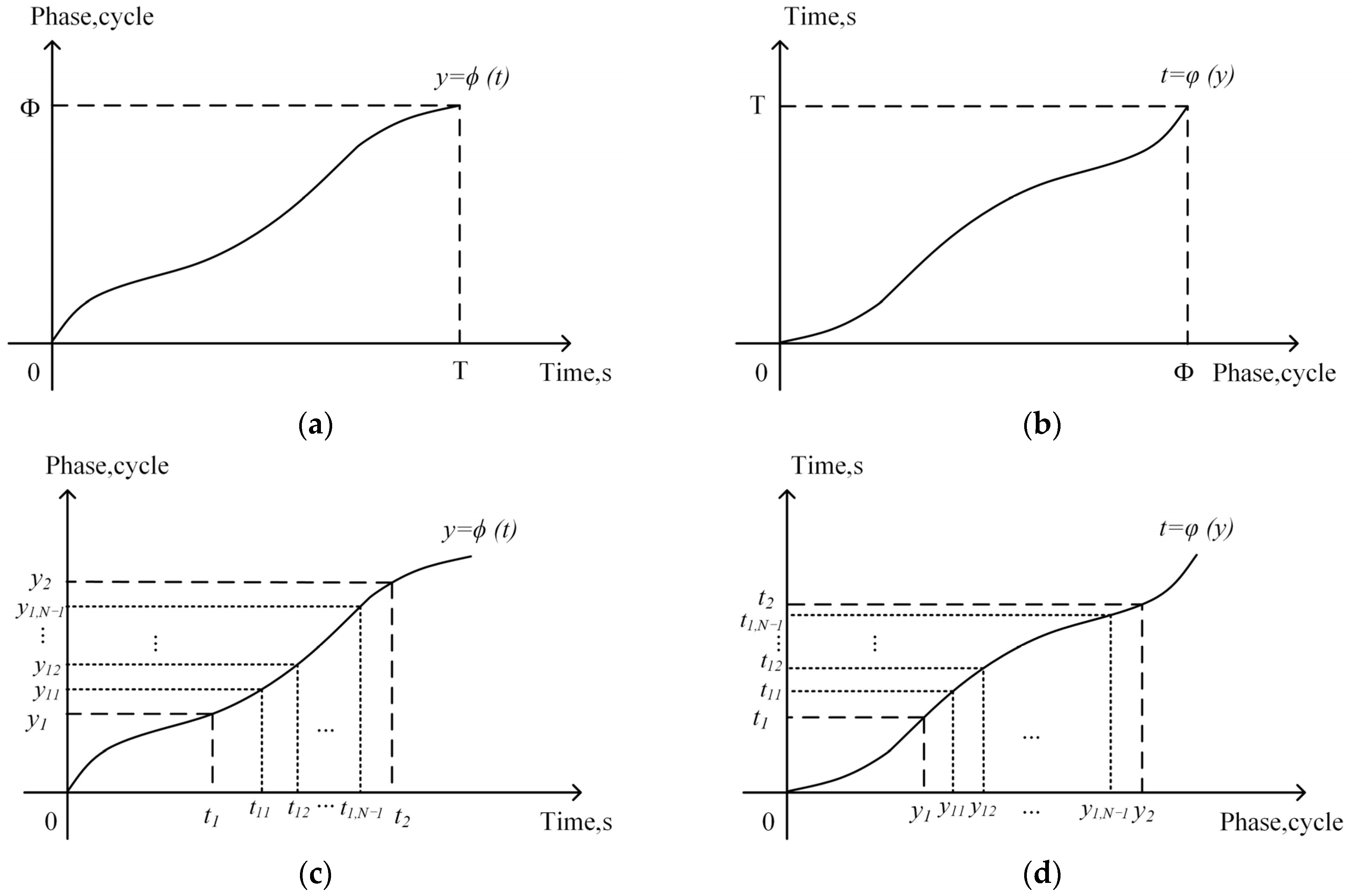
In order to further speed up the resampling process, while retaining the shaft-speed variation fidelity in synchronous analysis, we have developed an approach to locating the synchronous timestamps based on the inverse function interpolation. In this technique, the instantaneous shaft speed is time integrated to obtain the instantaneous phase
, as shown in
Figure 3a. Assuming the shaft is rotating only in a single direction,
is monotonic in
. Here we assume
and
for simplicity of statement. The inverse function
exists, and is also monotonic in
as shown in
Figure 3b.
In the instantaneous phase domain, the physical meaning of the synchronous timestamps is easily understood. As seen in
Figure 3c, for a given full shaft rotation cycle,
and
are the time marks of two adjacent key-phasor pulses (relative whole-revolution time marks in the tacholess analysis). The corresponding instantaneous phases at time
and
are
and
, respectively. Synchronous resampling means dividing
segments equally between
and
to form
, where
and
, and then determine
, where
and
. In other words, the synchronous resampling process is to find the independent variable points for given dependent variable points in the instantaneous phase function. The discrete timestamps,
, can be solved one by one according to the following equation
Solving Equation (6) usually requires an iterative process, which is expected to be a time-consuming numerical operation. With the inverse function known, as shown in
Figure 3d, the synchronous resampling timestamps are simply dependent variable data points evaluated at the inverse function by given independent variable data points
. For given
the synchronous resampling timestamps are evaluated at the inverse function
; and therefore,
In short, in numerical operations, evaluating the independent variable value for a given function value is often a time-consuming iterative process. Evaluating the function value for a given independent variable is a much simpler function valuation or interpolation process, and thus is much less time consuming. In rotating machinery signal processing, as long as the rotation direction of the shaft is unchanged, the instantaneous phase is a monotonic function with time. Its inverse function exists and is also monotonic. Therefore, we can always use the inverse function of the instantaneous phase to evaluate the synchronous resampling timestamps to improve data processing speed. In addition, since there is no approximation in the inverse function evaluation process, it is expected that the synchronous resampling based on the inverse function of the instantaneous phase will be more accurate.
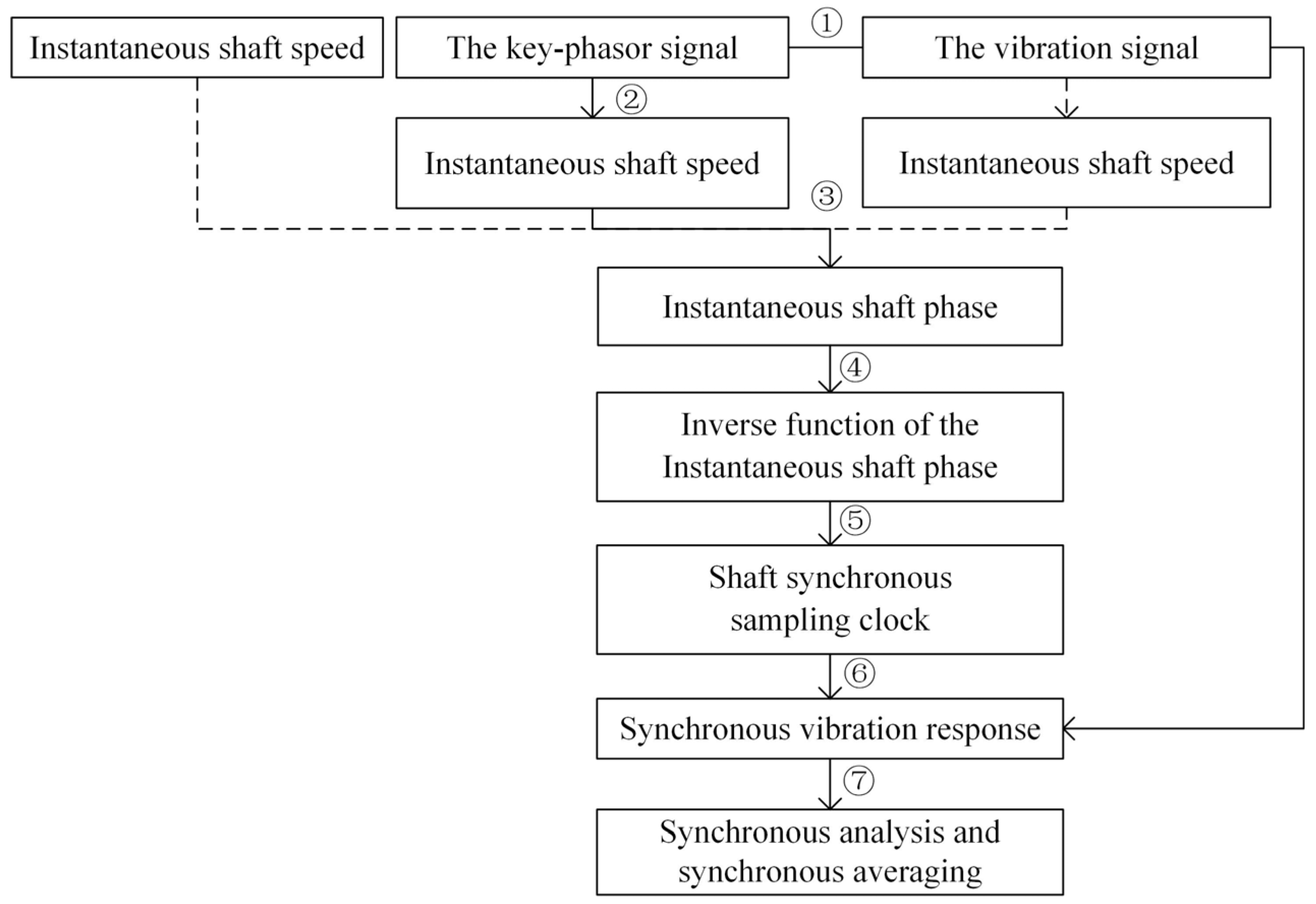
2.3. Implementation of Synchronous Resampling Based on Inverse Function Interpolation
Synchronous resampling based on inverse function interpolation can be implemented as shown in
Figure 4:
Signal acquisition. It is assumed that both the vibration signal and the key-phasor signal are obtained simultaneously and are digitized at a high sampling frequency with high resolution, as shown in
Figure 1.
Instantaneous shaft speed recognition. If the shaft speed information is provided in the form of a pulse train, the corresponding instantaneous shaft speed can be obtained by conventional signal processing [
25]. The instantaneous shaft speed can also be extracted by processing the vibration signal if the shaft speed information is not available [
26,
27].
Instantaneous phase recognition. Relative instantaneous phase function is obtained by numerical integration of the instantaneous shaft speed. Without losing the generality, the phase is set to 0 at initial time. The obtained relation between the phase of shaft rotation and time,
, is as shown in
Figure 3a.
Inverse function conversion of the instantaneous phase. Find the inverse function of the instantaneous phase identified in step 3, as shown in
Figure 3b.
Shaft synchronous resampling clock evaluation. Using the interpolation algorithm on the inverse function , the synchronous resampling timestamps , are determined quickly by evaluation from the inverse function for given .
Vibration response resampling. According to the synchronous sampling clock, the vibration response signal is resampled synchronously to obtain the synchronous response signal in the equal shaft angle domain.
Synchronous analysis and synchronous averaging. The synchronously resampled vibration response signal is analyzed and the results are used to diagnose the health condition of the rotation machinery.
3. Validation
This section verifies the feasibility and advantages of the proposed method through numerical simulations. Since data processing time is computer hardware- and software- dependent, the following lists the computer environment used in the simulations: Windows 10 Professional 64-bit operating system; MATLAB R2021b; 16 11th Gen Intel(R) Core (TM) i7-11700K @ 3.60 GHz; and 16 GB RAM.
In the numerical simulation, it was assumed that the shaft speed varies, as shown in
Figure 5a. In actual situations, the shaft speed information is obtained from the key-phasor, or evaluated from the measured vibration signal through instantaneous frequency identification techniques [
31].
For simplicity, the vibration response simulated here only contained the first-order response of the shaft rotation. Both the speed signal and the vibration response signal were digitized at 10,000 Hz. The signals lasted for 1000 s. The first 10 s of the signal time history is shown in
Figure 5b.
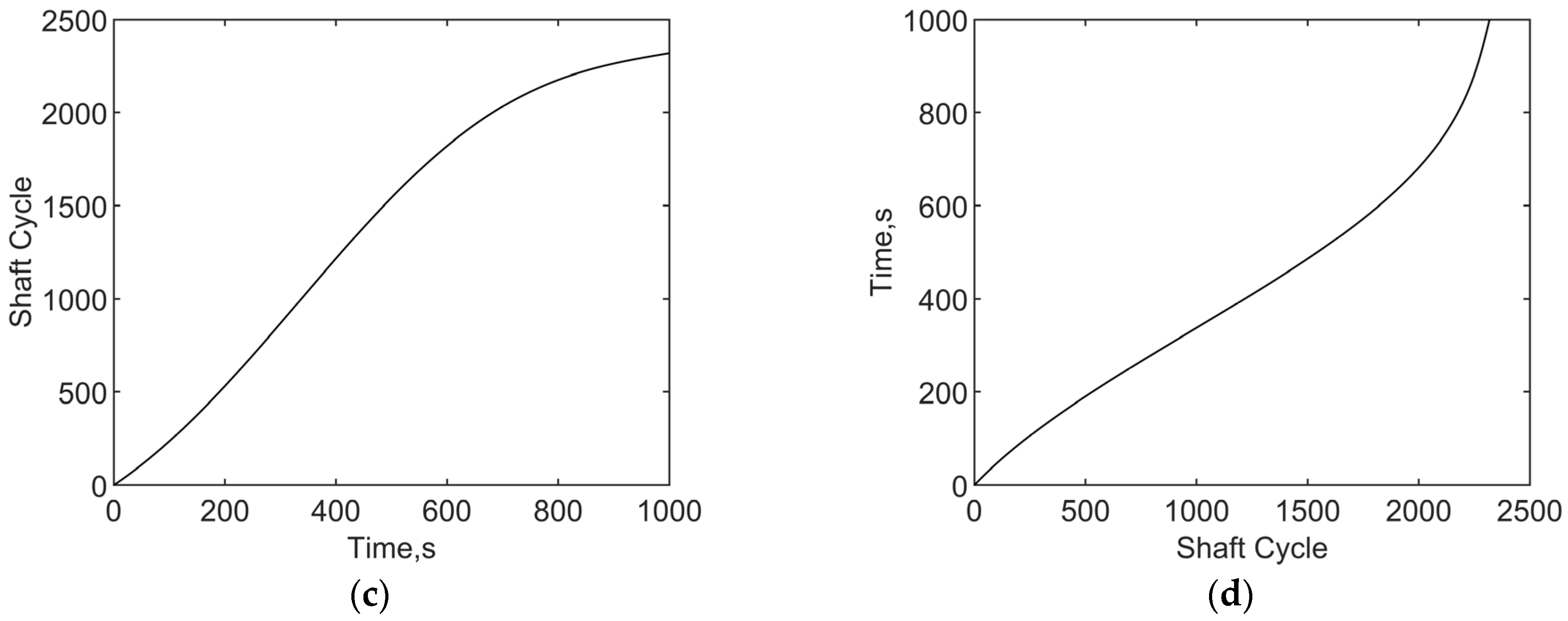
Before synchronous resampling, the instantaneous phase of the shaft was obtained by numerical integration of the identified shaft speed, as shown in
Figure 5c. The corresponding inverse function is shown in
Figure 5d. According to the highest shaft order required in the analysis, the synchronous resampling points within a shaft cycle were determined. In other words, the independent variable discretization points were specified for the inverse function of the instantaneous phase. An interpolation method can be applied to calculate the corresponding synchronous resampling timestamps. With the synchronous resampling timestamps, the equal delta time vibration response was converted to equal delta shaft angle synchronous vibration response by an interpolation algorithm.
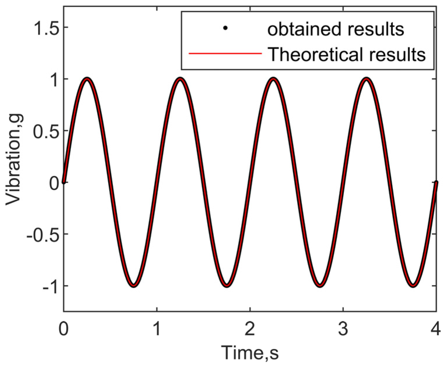
The first four cycles of synchronous responses are shown in
Figure 6. The performance of three synchronous resampling methods is listed in
Table 1, where the accuracy was measured by the mean squared error (MSE):
where
is the theoretical value of simulation, and
is the estimated value with different method.
In this simulation, for all the methods tested, the accuracies of the synchronous resampling were very high as expected, due to the mild speed variation in this simulation. However, the data processing efficiency of the inverse function evaluation-based method has been significantly improved. As seen in
Table 1, the processing time of the inverse-function-based method was about 37% of that used by the constant shaft-speed-based method, and was only about 17% of that used by the conventional iteration-based method.
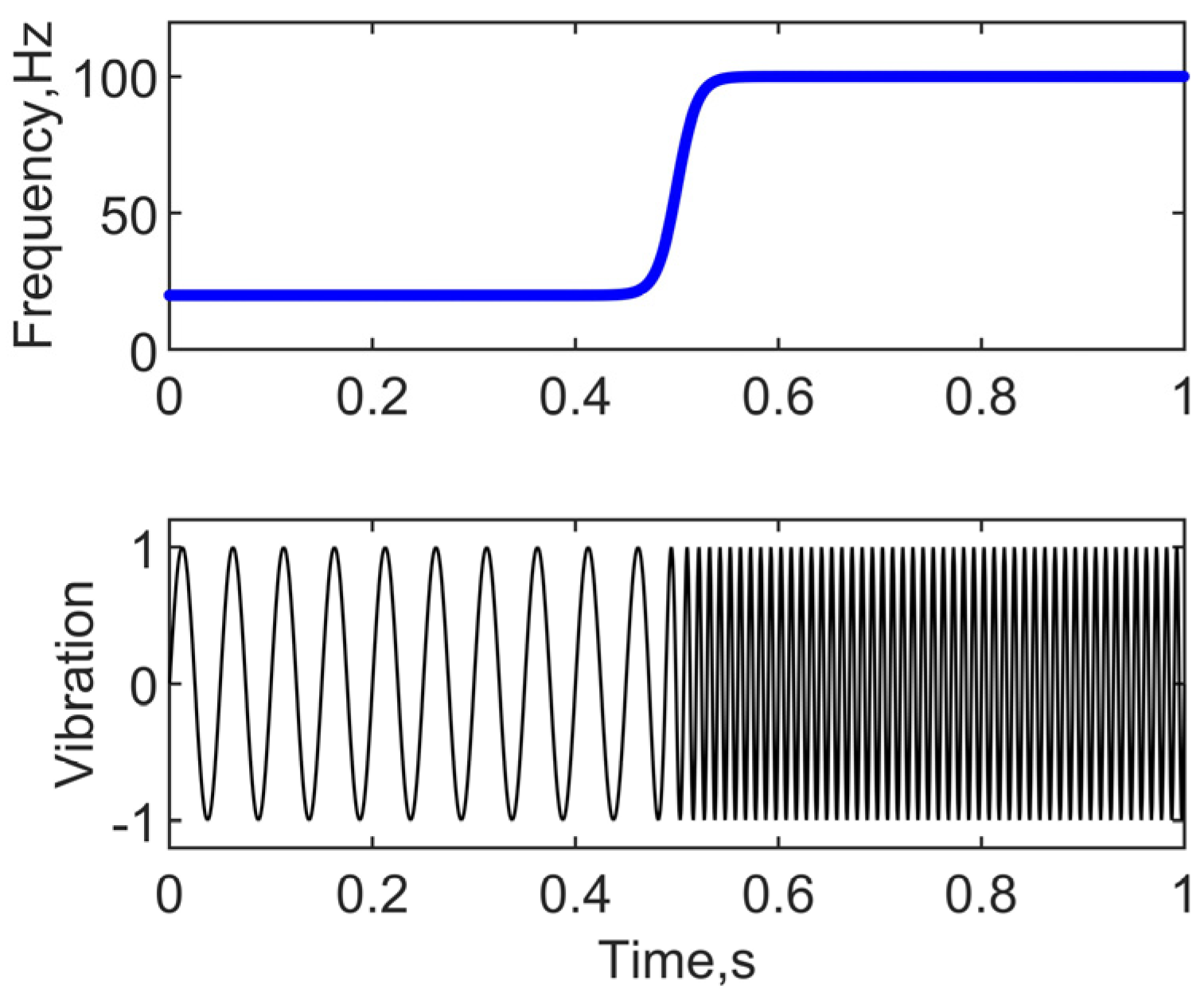
In order to further verify the accuracy of the proposed method, a case with more drastic shaft speed variation was simulated. The frequency variation is assumed to be:
where
and
are the frequency range and
is associated to the frequency change rate. The larger the
, the shorter the time required for the shaft rotation frequency to change from
to
. A case with
,
, and
is shown in the top portion of
Figure 7, and the corresponding vibration is shown in the bottom portion of
Figure 7.
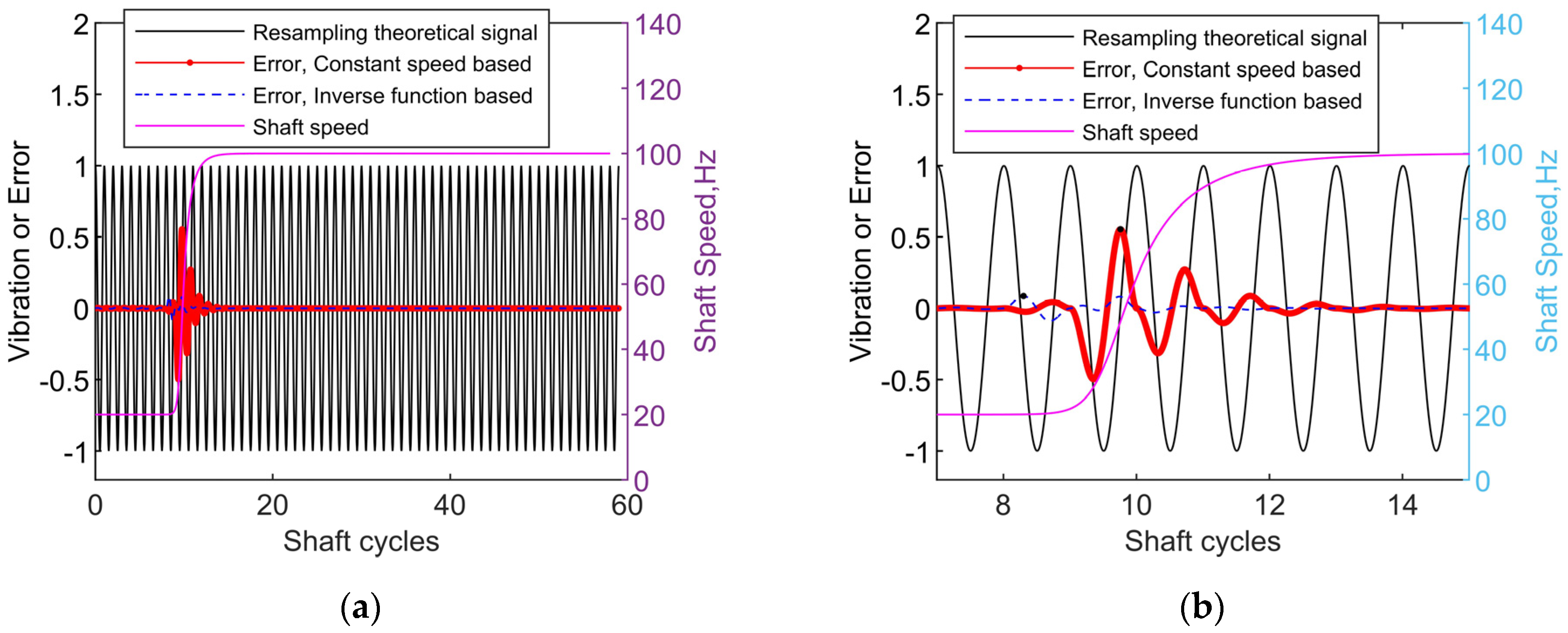
Digital signal processing was carried out with the same procedures as the previous example. The accuracy comparison of different resampling methods is presented in
Figure 8a. A zoomed version for the rapid speed change portion is shown in
Figure 8b. According to the simulation results, we were able to observe that, in the range of rapid shaft speed change, the method proposed in this study indeed rendered higher accuracy than that of the approximation method with the assumption of constant speed within a shaft cycle. For the current simulation case, the maximum error rate (the maximum amplitude difference vs. the simulated amplitude) of the constant frequency assumption (red line) was as high as 55.5%, while the maximum error rate from the proposed inverse function-based processing (blue dashed line) was less than 9%. The maximum errors for the different changing rate
were also evaluated and listed in
Table 2. As expected, the higher the speed change rate, the more maximum error was introduced in the constant speed-based method. The inverse function-based method accomplished consistently better results than those from the constant speed-based method.
5. Conclusions
Synchronous analysis technique is a very important tool in rotating machinery signal processing, especially in the damage detection and condition monitoring of bearings and gears. For variable-speed rotating machinery signal processing, the shaft speed synchronous resampling and the subsequent synchronous analysis is an effective way to improve the signal-to-noise ratio in signal processing.
Traditional digital-domain synchronous resampling timestamp computation is a time-consuming process, although it can speed up processing with certain approximations, such as the constant speed assumption within a cycle of shaft revolution. Sometimes it is still not sufficiently fast in processing long-time data or in applications with a quasi-real-time requirement. The proposed inverse function-based resampling algorithm replaces the time-consuming iterative procedure with a dependent variable evaluation procedure. Numerical simulations demonstrated that the proposed procedure improves the data processing efficiency as well as the accuracy significantly. Experimental tests also demonstrated that the proposed procedure is able to significantly improve the SNR of the damage feature extraction.
The implementation of the inverse function-based synchronous resampling algorithm is expected to significantly speed up synchronous processing. This makes the synchronous analysis algorithm more suitable for engineering applications in the condition of monitoring rotating machinery. In addition, it will improve synchronous resampling accuracy, especially in cases with rapid shaft speed variations.
However, the accuracy of this method depends on the accuracy of shaft speed identification. Any error in the shaft speed identification will be accumulated and propagated with time. How to achieve high-accuracy identification of shaft speed, and thus eliminate the cumulative phase error for a long-time data series, is still a challenging task.


 ,
, 


