Brake Disc Deformation Detection Using Intuitive Feature Extraction and Machine Learning

Abstract

In this work we propose proof-of-concept methods to detect malfunctions of the braking system in passenger vehicles. In particular, we investigate the problem of detecting deformations of the brake disc based on data recorded by acceleration sensors mounted on the suspension of the vehicle. Our core hypothesis is that these signals contain vibrations caused by brake disc deformation. Since faults of this kind are typically monitored by the driver of the vehicle, the development of automatic fault-detection systems becomes more important with the rise of autonomous driving. In addition, the new brake boosters separate the brake pedal from the hydraulic system which results in less significant effects on the brake pedal force. Our paper offers two important contributions. Firstly, we provide a detailed description of our novel measurement scheme, the type and placement of the used sensors, signal acquisition and data characteristics. Then, in the second part of our paper we detail mathematically justified signal representations and different algorithms to distinguish between deformed and normal brake discs. For the proper understanding of the phenomenon, different brake discs were used with measured runout values. Since, in addition to brake disc deformation, the vibrations recorded by our accelerometers are nonlinearly dependent on a number of factors (such as the velocity, suspension, tire pressure, etc.), data-driven models are considered. Through experiments, we show that the proposed methods can be used to recognize faults in the braking system caused by brake disc deformation.

1. Introduction

Vehicle manufacturers prioritize safety as a paramount concern. This is well reflected in the fact that automobile manufacturers place emphasis on the design of reliable and easy-to-maintain parts when introducing new vehicles. Despite this, the degradation of vehicles is inevitable over time; moreover, the rate of decline can be difficult to estimate. This is especially true if the vehicle was operated in extreme conditions or in a manner not anticipated by the manufacturer. One of the most safety critical subsystems in a vehicle is the braking system. Unmaintained and damaged brakes frequently lead to accidents. In fact, according to [1], faults in the tire and braking system were the most important factors contributing to accidents due to mechanical defects of the vehicle. Furthermore, in [2], it is shown that the likelihood of brake system failure significantly increases with the age of the vehicle. In addition, many types of brake system faults are actively monitored by the driver or the passengers of the vehicle. Thus, these types of faults may not be recognized in fully autonomous modes of operation. For these reasons, the continuous and automatic monitoring of possible faults in the braking system is necessary.

Such monitoring schemes are usually realized through fault-detection methods [3]. Brake system fault-detection approaches have been proposed in several previous studies [4,5,6,7,8]. In [4], a thorough review of fault-detection methods designed specifically for heavy vehicles (such as trucks) using air brakes is provided. Novel approaches based on vibration signals obtained from experimental setups in a laboratory were proposed in [5,6]. For [5,6], vibrations signals were obtained from piezoelectric accelerometers built into the experimental setup. The above-mentioned studies focused on detecting faults in the braking system in a general sense. In [7], it is pointed out that focusing on identifying a specific type of fault increases the performance of detection methods. For this reason, a method capable of detecting frictional faults of the disc brake was studied and verified through simulations in [7]. Using laboratory conditions, further novel methods were introduced in [8] to recognize frictional brake disc faults from vibration signals. Finally, it is worth noting that similar fault-detection algorithms were proposed for disc brake systems which are not operated in passenger vehicles. In particular, the brake system fault detection of mine hoists has been a well-studied problem [9,10].

The relationship that describes the connection between frictional brake disc faults and measured vibration signals is highly nonlinear [8]. In addition, the vibration signals are non-stationary [6,8]. For these reasons, most recent studies [5,6,7,8] rely on data-driven machine learning (ML) methods [11,12] instead of classical approaches [3] to detect faults in the brake system. Even though ML approaches are able to handle the nonlinear and non-stationary nature of the problem, their behavior is often non-interpretable to humans [13]. This is especially true when deep neural networks and so-called convolutional neural networks [12,13,14,15] are used.

The main contribution of this study is a novel measurement system consisting of a physical part and signal-processing part. The proposed system is capable of detecting frictional brake disc deformations, also referred to as brake disc runout. The physical part includes several acceleration sensors mounted to certain points of the vehicle and corresponding readout electronics. The signal-processing part consists of ML algorithms whose effectiveness is verified on measurement data. The proposed measurement system constitutes a novel improvement on previous methods because of the reasons detailed below.

Firstly, the proposed system is verified using measurements from a real vehicle instead of ones obtained in laboratory conditions. This represents a higher technology readiness level (TLR) [16] than most recent studies [4,5,6,7,8], as the results presented in this paper are verified on data obtained from the relevant environment instead of the laboratory. In the proposed setup, the algorithms and equipment need to be robust against vibrations introduced by the tires, the suspension and various other factors not present in laboratory conditions.

Another major advantage of the current study is that the investigated ML methods were chosen to satisfy requirements commonly associated with the automotive industry. An emphasis is placed on the development of intuitive feature-extraction transformations instead of using large end-to-end models [6,8] to increase the interpretability of the results. In addition, all considered algorithms (including the investigated convolutional neural networks) were selected in a way that allows for implementation on inexpensive hardware such as microcontrollers and field programmable gate arrays (FPGAs) similarly to the authors’ previous works [17,18]. The light-weight nature of the proposed models allows for the reduction of production costs in future realizations of the proposed system.

The rest of this paper is organized as follows. Section 2 contains information about the physical part of the proposed measurement system, the test vehicle and the measurement scenarios. In Section 3, the behavior of the obtained signals is detailed. This discussion is later used to construct appropriate ML methods and corresponding feature-extraction schemes for brake disc fault detection. Section 4 poses the question of fault detection as a supervised learning problem and proposes several intuitive feature transformations. In Section 5, the conducted experiments, model specifications and discussions are provided. Finally, Section 6 contains conclusions and future plans.

2. Measurement Setup

2.1. Brake Disc Deformations

The hydraulic brake system uses fluid pressure to transmit force from the brake pedal to the brake pads. When the pedal is pressed, brake fluid amplifies the pressure, causing the pads to clamp onto the brake discs or drums, effectively slowing or stopping the vehicle. Brake disc runout or vibration is caused by a fault in one or more components of the braking system. The phenomenon is mainly observed through a “hitting brake disc” effect, when the brake pedal is fully pressed. In worse cases, strong vibrations are felt on the steering wheel or the whole vehicle. These vibrations can be felt as a passenger sitting in the front or the back of the vehicle, depending on the position of the wheel with the deformed brake disc. The phenomenon may also be accompanied by a strong frictional sound effect. The aggravation of brake disc hitting can be very disturbing and is likely to affect the length of the braking distance, which can lead to accidents. Its detection is therefore very important and measurements are needed to better understand the practical effects of this phenomenon. Since this type of damage is usually detected by the driver of the vehicle, in autonomous driving modes, it is important to develop methods to detect brake disc runout automatically. Self-diagnostic systems are essential for safety and proper maintenance. The most common cause of vibrations are changes in the thickness of the brake disc. For this reason the term “brake disc wobble” is also frequently used to describe this phenomenon. The differences in the degradation of the brake disc surface can be caused by a variety of factors. For example, uneven brake pad wear or dirt wedged between the braking surfaces are both common causes. In the latter case, the pad consumes the brake disc unevenly when braking. Another cause could be a faulty brake disc from the factory, such as a brake disc with imperfect geometry. A very extreme example of brake disc deformation is shown in Figure 1, where inclusions are found in the casting due to inadequate manufacturing and inspection conditions.

Imperfect geometry can also occur during use due to high temperatures under unplanned operating conditions which can result in brake disc burnout. It should be noted that, under normal operating conditions, the probability of brake discs reaching a temperature that would cause them to blister is very low. The threshold temperature for this to occur is above 500 °C. Geometric inaccuracies may not be detected without measuring before fitting, since a runout of up to $0.1$ mm can cause the brake disc to hit. This dimensional inaccuracy, however, is not visible to the human eye. Brake disc wobble can also occur if the surface is not properly prepared before the brake disc is fitted due to the presence of dirt or even rust on the hub or the brake disc. Furthermore, brake disc blow-outs can also be caused by an accident or a shock event (such as driving into a pothole) that causes a change in the geometry of the braking system. Another common cause is when the brake disc is fitted incorrectly, for example off-center on the hub or unbalanced. In some cases, wear in the running gear (such as ball joints or spacers) can also cause the problem.

2.2. Measurement Scenario

The platform on which the measurements considered in this study were carried out is the ZalaZONE (see, e.g., [19]) Brake Measurement Surfaces. This test track is specifically designed to carry out braking measurements. The total length of the test surface is 1100 m, the acceleration section is 750 m, the length of the braking surfaces is 200 m and there is a safety zone of 150 m. The width of each lane is $4.5$ m across all sections of the test track. There are eight braking surfaces with different coarseness levels (friction coefficients [20] range between $0.1$ and $1.0$) in the test area. A surface with a friction coefficient of approximately $1.0$ was chosen to conduct the measurements considered in this study.

The testing area allows for each braking surface to be optionally soaked; furthermore, some surfaces can only be used in wet conditions with a maximum water height of 5 cm for “aquaplaning” tests. It is worth noting that the measurements for this study were conducted on dry surfaces.

In addition to the brake test surfaces, there is a 20 m wide skid bar on either side of the test track. The surface is designed to allow testing with a maximum vehicle weight of 40 tonnes. The braking surface zone is deliberately designed to be connected to the highway test area to ensure that more complex tests can be carried out. The braking surface provides the possibility of performing both normal vehicle dynamics tests and self-driving car/ADAS (Advance Driving Assisted Safety) [21] tests. The brake disc runout test was performed on a 2020 Volkswagen e-Golf, shown in Figure 2.

The measurements were carried out with two different brake discs, all mounted on the right front wheel. First, a factory brake disc with 15,034 km and $0.02$ mm of runout was considered. In each case, the brake disc runout was measured with a dial gauge, which was fixed using a magnetic stand. Figure 3 shows the dial gauge measurement of the factory brake disc.

In the second round of measurements a deliberately damaged brake disc was used. The $0.12$ mm runout damage was caused by drilling. The impacted brake disc in the mounted condition is shown in Figure 4. The stamped brake discs were of the Automotive Brake Engineering (ABE) brand.

The same brake pads were used for every measurement. Two measurements were conducted with each of the above-mentioned brake discs using a 2 bar tire pressure. As mentioned above, the measurements were conducted on a surface with a friction coefficient of approximately 1.0.

In each scenario, cruise control was used to achieve a maximum velocity of 100 km/h with the vehicle moving along a straight line. It is worth noting that, in reality, car manufacturers reset the speedometers on the dashboard by about 5 km/h to make it easier to comply with speed limits. This means that the actual top speed reached during the measurements was about 95 km/h in each test scenario. Upon reaching the maximum speed, emergency braking was applied to bring the vehicle to a complete halt. The braking maneuver began at approximately the same point in the test track for each measurement scenario. This type of measurement was performed a total of four times. The individual measurement scenarios are broken down as follows:

• Two measurements: factory used brake disc (15,034 km) with 2 bar wheel pressure;
• Two measurements: aftermarket, intentionally damaged brake disc (ABE type, ground) with 2 bar wheel pressure.

The brake disc deformations were measured with a dial indicator as shown in Figure 3. For the factory brake discs the measured runout was $0.02$ mm, while the deliberately made hammered disc had a runout of 0.12 mm.

Two software tools were used for measurement and evaluation purposes. PicoDiagnostics $v1.16.83$ by Pico Technology (Cambridgeshire, UK) was used to record the vibrations. The other software was Kvaser’s CanKing $v.3.9$ by Kvaser (Mölndal, Sweden), which was used to record velocity data and acceleration data in three axial directions based on GPS signals. To record the vibrations, the Pico Scope 4823, an eight-channel automotive oscilloscope, and two Pico NVH kits, three-axis accelerometers, were employed. Data collection from the accelerometers was performed using a sampling frequency of 20 KhZ. This equipment is illustrated in Figure 5.

Two accelerometer sensors were installed at the front passenger side wheel in a vertical orientation on the swingarm and the stub axle. The sensor on the swingarm is shown in Figure 6.

3. Signal Description and Preprocessing

In this section, the behavior and defining characteristics of the obtained signals are discussed. The 1-D acceleration signals were measured using the sensors mounted near the suspension of the vehicle as discussed in Section 2. In addition, information about the vehicle’s speed was also available, albeit in a much undersampled form (see Section 2). The purpose of this study was to provide proof-of-concept applications which can recognize the deformed brake discs based on the available signals; therefore, a general discussion on their behavior is necessary.

The most important assumption behind the proposed signal-processing methods is that brake disc deformations can be recognized based on the available acceleration signals. In other words, brake disc deformations manifest themselves as changes in the vibration characteristics of the vehicle’s suspension. In particular, since they can be viewed as sudden, so-called shock events (see, e.g., [22]), the vibrations caused by brake disc deformation should appear as additional high-frequency noise in the signals. For this reason, the mathematical concept of Fourier series and the (discrete) Fourier transform (see, e.g., [23]) is an important tool in our analysis of the signals. In order to develop methods which can detect the changes caused by a deformed brake disc, it is useful to discuss other factors which might cause changes in the vibration profile of the vehicle.

Since the wheels are engaged in periodic motion, changes in the velocity of the vehicle will affect the spectrum of the vibration signals. That is, as vehicle speed increases, higher-frequency components become more prominent in the vibration signals. This phenomenon is illustrated in Figure 7. Here, the magnitude of the discrete Fourier coefficients of two signal segments obtained from the same measurement are shown. In the first one (blue line), the vehicle’s mean velocity was 75 km/h, while the second signal segment (red line) corresponds to a mean velocity of 30 km/h. Clearly, increasing the velocity of the vehicle leads to the appearance of more dominant high-frequency components. Because of this non-stationary behavior, the detection methods proposed in Section 4 will not rely solely on the frequency space representation of the signals.

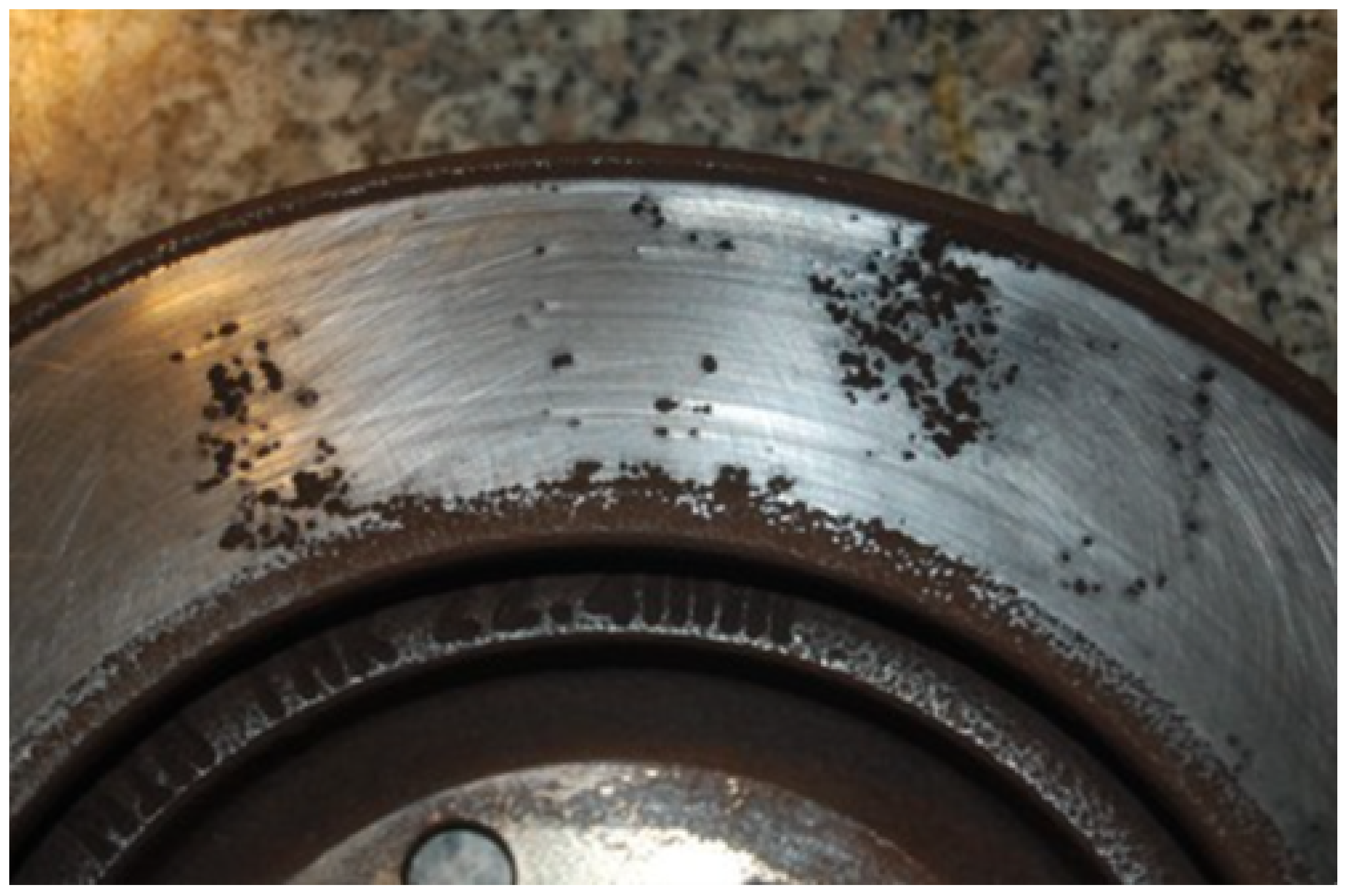
In addition to varying frequency profiles due to the changes in velocity, several difficulties need to be overcome for recognizing brake disc deformations. Firstly, regardless of speed, the signals contain noise, which leads to the appearance of high-frequency components in the spectrum. Due to this characteristic, the vibration measurements obtained with deformation-free and deformed brake discs are difficult to distinguish in the frequency domain. Another difficulty in deformation detection arises from the fact that the effects of brake disc deformation cannot be continuously observed throughout the signals. For example, the effects of this type of fault only appear in the measurements when the brakes are applied to the vehicle. In addition, the deformations may only cover a portion of the brake disc. In this case, their effect can only be observed when the deformed part of the disc makes contact with the brake pads during the braking process. For example, in the current measurement setup (see Section 2), deformations were modeled by a single indentation on the brake disc surface (see Figure 4).

For the above reasons, several preprocessing steps were conducted on the vibration measurements prior to the application of the investigated fault-detection methods. First, the portion of the signals was extracted where the brake pads were in use. Since no direct information was available about brake pedal (or brake pad) positions in the measurements, the parts of the measurement when vehicle speed was decreasing were cropped. More precisely, parts of the signals between a maximum (90 km/h) and a minimum (30 km/h) speed value were extracted while the vehicle was braking. The extracted parts of the accelerometer signals are illustrated in Figure 8. These cropped signal segments consisted of around $40,000$ useful data points for each measurement scenario.

In the experiments described in Section 5, measurements from four different measurement scenarios were used. Two scenarios used the artificially deformed brake disc, while the remaining two runs used the factory (deformation-free) brake equipment of the test vehicle. Because of the above-described properties, the relationship between the measured vibrations and the presence of brake disc deformation is highly nonlinear. Thus, the examined fault-detection methods follow the data-driven paradigm (see Section 5.1). The main benefit of data-driven methods is that they can be used to accurately model nonlinear functions based solely on data [11,12]. However, in order to achieve optimal performance, these types of methods require an abundance of input data [11,12]. For this reason, a further segmentation of the cropped signals (in Figure 8) was needed.

The presence of a deformation can only be observed in the signals when the brake pads are pressing directly against a deformed part of the brake disc. Thus, in order to ensure that each signal segment can be used to detect a potential deformation, each segment had to contain data corresponding to at least one full wheel revolution. Unfortunately, the current test vehicle was not equipped with an accurate wheel angle measuring apparatus; therefore, segmenting the measurements to single wheel revolutions was not possible. Instead, the presence of full revolutions in each segment was ensured using the following methodology. The test vehicle was equipped with R16 size tires for the measurements. These types of tires have a circumference of ∼2.5 m, which (since the vehicle was traveling in a straight line) coincides with the distance traveled during a single wheel revolution. Using this information and the sampling frequency of the vibration signals, it was possible to determine the time T needed for a single wheel revolution when the vehicle was traveling at the lowest speed still considered (for this study 30 km/h). Segmenting the signals into T-length time intervals ensured that each signal segment contained at least a single full tire revolution. Using this strategy, each signal segment contained vibrations caused by brake disc deformations if they were present. In this way, the signals from each measurement could be divided into a number of segments to increase the amount of data for the proposed processing methods discussed in Section 5.1. It was possible to further increase the number of available signal segments by using overlapping windows (see Section 5 for specifics).

4. Deformation Detection Methods

Formally, the detection of brake disc deformations can be given as the identification of the operator $F:{\mathbb{R}}^{4\times N}\to \{0,1\}(N\in \mathbb{N})$, where N denotes the number of sampling points in the segmented signals and 4 is the number of accelerometers used. Suppose that $F\left(x\right)=1$ if x was measured with brake disc deformations present in the vehicle and $F\left(x\right)=0$ otherwise. This operator is highly nonlinear because of the reasons discussed in Section 3. The problem of detecting brake disc deformations is equivalent to approximating the operator F. Because of the nonlinear behavior of this operator, however, conjuring an analytic model (see, e.g., [3]) of F is difficult. Furthermore, most classical fault-detection methods [3] assume stationary input signals. Because of the reasons discussed in Section 3, the measurements in this study cannot be considered stationary. Thus, in this paper, instead of analytic models, data-driven methods are investigated. More specifically, so-called supervised learning (SL) methods (see, e.g., [12]) are considered. A general overview of SL methods is provided in this section.

In the context of brake disc deformation detection, a formalization of SL methods is introduced here. Let $\mathcal{X}\subset {\mathbb{R}}^{4\times N}$ denote the set of all possible signal segments. The objective of SL approaches is to identify a parametrized model

$$G_{\theta }:\mathcal{X}\to \{0,1\},(\theta \subset {\mathbb{R}}^M,M\in \mathbb{N}),$$

for which $F\approx G_{\theta }$. This notion of “closeness” is usually evaluated using a so-called “loss function” $E:\{0,1\}\times \{0,1\}\to [0,\infty )$. That is, the objective of SL methods is to find the parameter vector $\theta$, for which the expression

$$r\left(\theta \right):=\sum _{x\in \mathcal{X}}E(F\left(x\right),G_{\theta }\left(x\right))$$

(1)

is minimized. Since, for brake disc fault detection, the range of F is the discrete set $\{0,1\}$, the models $G_{\theta }$ will be often referred to as “classifiers” and the approximation problem as a “classification task”.

In practice, it is only possible to record a finite amount of signals. Let $\mathcal{T}\subset \mathcal{X}$ denote the set of available segmented measurements. Minimizing $r\left(\theta \right)$ from (1) over $\mathcal{T}$ is usually not preferable because of the phenomenon of so-called overfitting (see, e.g., [12]). That is, for a sufficiently sophisticated model $G_{\theta }$, the solution of (1) over $\mathcal{T}$ might yield a result where the model is very precise for signals in $\mathcal{T}$, but may be unreliable for accelerometer signals where $x\in \mathcal{X}$ and $x\notin \mathcal{T}$. In order to address this issue, before solving (1) (a process also known as “training”, see, e.g., [12]), the set of preprocessed measurements $\mathcal{T}$ is split into two, non-overlapping subsets:

$$\mathcal{T}:={\mathcal{T}}_{tr}\cup {\mathcal{T}}_{te}{\mathcal{T}}_{tr}\cap {\mathcal{T}}_{te}=\varnothing .$$

(2)

In (2), the set $T_{tr}$ is referred to as the “training” set, while $T_{te}$ is referred to as the “test” set. In order to avoid overfitting, the model $G_{\theta }$ is trained over $T_{tr}$ only, that is, the nonlinear optimization problem (1) is only considered over $T_{tr}$. Then, once an optimal $\theta$ has been determined, the generalization properties of the model are measured by evaluating

$$\sum _{x\in {\mathcal{T}}_{te}}E(F\left(x\right),G_{\theta }\left(x\right)).$$

The models $G_{\theta }$ (and the corresponding strategies to solve the approximation problem) used in this paper are detailed in Section 5.1. Although many different strategies (models) exist to solve SL problems [11,12], certain common properties are worth pointing out here. Even though SL models have achieved important breakthroughs in many different nonlinear modeling problems such as image-processing [24], biological signal-processing [25,26,27] and engineering applications [6,8,18,28], their use incurs certain costs. Firstly, many models, especially popular so-called neural networks (see, e.g., [12] and Section 5.1), require large amounts of data to provide a good approximation of F. In addition, the optimized model parameters $\theta$ are often not interpretable by humans, making the application of SL models challenging in a number of disciplines.

In order to remedy the lack of interpretability of SL methods, several strategies can be employed [12]. For example, some SL models, such as the support vector machine (SVM) (see, e.g., [29]), contain parameters which retain certain geometrical meaning. Another useful method to improve the interpretability of SL methods is to employ so-called feature-extraction transformations [12,25]. In the case of brake disc deformation detection, feature-extraction transformations can be described as operator $\mathrm{\Psi }:{\mathbb{R}}^{N\times 4}\to {\mathbb{R}}^K(K,N\in \mathbb{N})$. This operator is applied to every available measurement in $\mathcal{T}$ to create a new, transformed set of extracted features:

$${\mathcal{T}}^{\prime }:=\{\mathrm{\Psi }\left(x\right):x\in \mathcal{T}\}.$$

(3)

The exact definition of $\mathrm{\Psi }$ depends on the task at hand; therefore, the application of feature-extraction transformations allows for a degree of interpretability. In addition, transformations which reduce the dimension of the input data and capture important statistical properties of the measurements have been shown to reduce overfitting [12].

In the case of brake disc deformation detection, the following intuitive feature-extraction transformation was applied. Since deformations of the brake disc are assumed to manifest themselves as added noise on the measurements, the standard deviation of the measured signals can capture this phenomenon. More precisely, the feature extraction $\mathrm{\Psi }:{\mathbb{R}}^{N\times 4}\to {\mathbb{R}}^4$ was investigated, where

$$\mathrm{\Psi }{\left(x\right)}_i:=\sqrt{\frac{1}{N-1}\sum _{k=1}^N{|\overline{x_i}-x_{k,i}|}^2}(i=1,\dots ,4),$$

(4)

where $\overline{x_i}:=\frac{1}{N}{\sum }_{k=1}^N{x}_{k,i}$ denotes the mean of the measured acceleration data from the i-th sensor. As shown in Section 5, the introduction of transformation (4) significantly improved model accuracy for the investigated SL methods.

In addition to the intuitive feature-extraction scheme (4), in this paper, the popular principal component analysis (PCA) (see, e.g., [30]) was also considered. PCA has been shown to be a very effective feature-extraction transformation, able to capture meaningful information about the data while reducing its dimensions. The intuition behind PCA can be expressed as follows. Consider a random vector $v\in {\mathbb{R}}^d(d\in \mathbb{N})$. PCA attempts to find an orthonormal basis $e_1,\cdots ,e_d$ and project v onto the subspace spanned by the vectors $e_1,\cdots ,e_d$. The first coordinate of the acquired transformation should correspond to the maximal variance of any scalar projection of v, the second coordinate should correspond to the second greatest variance orthogonal to the previous one and so on. These coordinates are referred to as “principal components” of v. Formally, in the context of brake disc fault detection, consider the measured acceleration signal segments $x\in {\mathbb{R}}^{N\times 4}$ as realizations of independent, identically distributed random variables. Then, the (empirical) principal components corresponding to x can be expressed as

$$\mathrm{\Psi }{\left(x\right)}_i:={\left(Ux\right)}_i(i=1,\dots ,4),$$

(5)

where the matrix U is acquired from the singular value decomposition (see, e.g., [30]) of the signals: $x=UD{V}^T$.

Even though the application of transformations (4) and (5) provide a degree of interpretability, these representations of the acceleration signals may not be optimal. Many modern machine learning methods use the notion of automatic feature extraction instead of static transformations such as (4) and (5). Automatic feature extraction can be formalized for brake disc fault detection as ${\mathrm{\Psi }}_{\eta }:{\mathbb{R}}^{N\times 4}\to {\mathbb{R}}^K,(\eta \in {\mathbb{R}}^M,K,N,M\in \mathbb{N})$. In other words, the feature-extraction transformation depends on the parameter $\eta$. The main advantage of machine learning methods which employ automatic feature extraction is that the feature-extraction parameter $\eta$ is trained together with the $\theta$ parameters of the underlying SL model $G_{\theta }$. Convolutional neural networks (CNNs) follow this paradigm, that is, the first few layers of CNNs implement discrete convolutions which can be interpreted as feature-extraction transformations (see, e.g., [15]). In general, neural networks can be interpreted as nested (linear and nonlinear) mappings of the input data, which depend on certain parameters [12]. For CNNs the feature-extraction parameters $\eta$ make up the values of the convolution kernel [15]. In Section 5, it is shown that CNNs can also be effectively used to recognize brake disc deformations.

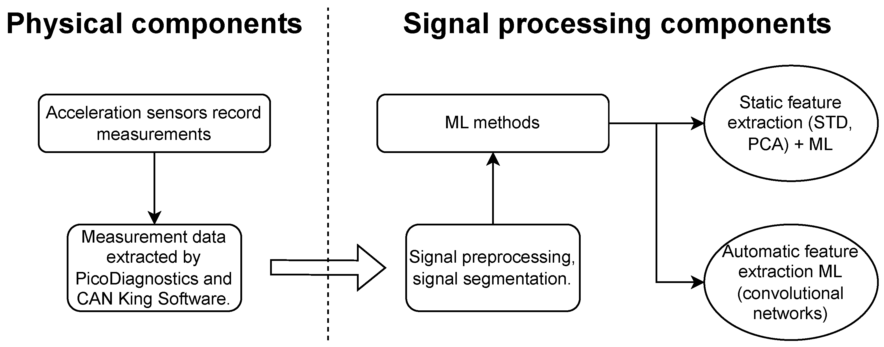
In summary, this study is a proof of concept demonstrating that brake disc deformations can be detected using several machine learning methods. The exact model specifications are provided in Section 5.1. In addition to investigating different ML models, intuitive analytic (see Equation (4)) and automatic (via CNNs) feature-extraction scenarios were also considered. The application of analytic feature extraction allows for a higher degree of interpretability, while CNNs provide more adaptive data representations. Model performance comparisions are discussed in detail in Section 5.2. A schematic of the proposed measurement system is given in Figure 9. It consists of the physical components discussed in Section 2 followed by the ML-based signal-processing component encompassing a variety of algorithms. All of the considered ML algorithms follow the paradigms discussed in this section.

5. Experiments

The experiments in this study were built around the measurements discussed in Section 2. The measured acceleration signals were segmented and preprocessed according to the steps provided in Section 3. That is, each signal segment was guaranteed to contain data from at least one full tire revolution and all signal segments were recorded during active braking with vehicle speed remaining between 90 and 30 km/h. In the current measurements this resulted in signal segments from a single accelerometer consisting of 6123 data points. Altogether, four measurement scenarios were considered. As explained in Section 2, the vehicle accelerated along a straight line followed by intensive braking. Each measurement was recorded on the same road surface and, for the considered measurements, the tire pressure was fixed at 2 bars. In two of the considered measurements the vehicle was equipped with artificially deformed brake discs, while in the remaining two measurements the undamaged stock brake discs were used. The preprocessed data segments were labeled according to which measurement they were extracted from.

Two different datasets were created from the measurements. In the first case, all four measurements were segmented with no overlap (in time) between the segments. In this case however, the four measurements yielded a total of 22 segments, which is not enough to efficiently employ large data-driven models. For this dataset, a five-fold cross-validation [11,12] scheme was used to evaluate the performance of each investigated model. In this experiment, the dataset was divided into five subsets and each investigated model was trained and tested five times. In each of these training and testing steps (also known as folds), a different subset was used to test the model’s generalization properties and the remaining data were used for training. The performance results from each fold were averaged to provide a more robust and representative estimate of the model’s generalization performance. It is worth noting that for the experiments detailed in this manuscript the subsets were created in a balanced manner, that is, the ratio of deformed and normal signals remained the same in each subset (see

Table 1. Number and ratio of signals in the two considered datasets.

Dataset	# of Deformed Signals	# of Normal Signals	Total # of Signals
Non-overlapping	12 (∼55%)	10 (∼45%)	22
Overlapping	$3279(50\%)$	$3279(50\%)$	6558

for the ratios).

In order to retrieve more signals from the available measurements, the second dataset was created by extracting overlapping signal segments. In this case, instead of five-fold cross-validation, a single training of each model was considered. To ensure that no data leakage occurs due to the overlapping nature of the segments, the training and test sets were created from different measurements. The segmentation method used to create the different datasets is illustrated in Figure 10. The total amount of signal segments obtained from the first and second datasets is given in Table 1. In these experiments, an overlap of 6113 data points was used for the training set and an overlap of 6023 was used for the test set. Considering the sampling frequency detailed in Section 2, this constituted an overlap of approximately $0.3$ seconds for both sets.

According to Table 1, both datasets contained roughly the same amount of deformed and normal signals. For this reason, model performance was evaluated using the accuracy metric:

$$Acc:=\frac{TP+TN}{P+N},$$

(6)

where $TP$ and $TN$ denote the number of true positive and true negative model predictions, and P and N denote the total number of positive (deformed) and negative (normal) signal segments, respectively. A model prediction for the input signal x is considered true positive if $G_{\theta }\left(x\right)=1=F\left(x\right)$, where the label $F\left(x\right)$ is known explicitly. In the experimental results provided in Section 5.2, the presented accuracy scores always refer to the model’s accuracy achieved on the test set.

5.1. Data-Driven Models

In this section, the realizations of the considered machine learning models are detailed. Several well-known ML approaches were used in the proposed experiments in order to obtain a robust overview about the behavior of the recorded signals. In addition, experiments with a number of models provide a solid proof of concept that using the proposed measurement system allows for the detection of brake disc deformations. Furthermore, examining the effect of different algorithms strongly supports future research on the proposed measurement system and provides insight into which ML methods should be considered for use in a commercial realization. The hyperparameters of the considered models were set by an extensive search of the corresponding hyperparameter space. Every considered experiment was implemented in the python programming language using the scikit-learn [31] and pytorch [32] libraries.

The first investigated ML model in this study was a linear support vector machine [17,29]. This type of classification algorithm attempts to find a hyperplane which optimally separates the data (2) by class labels. Finding the parameters describing the optimal hyperplane is usually posed as the linear programming problem. Specifically, so-called soft-margin support vector classifiers were considered:

$$\begin{array}{cc}\hfill \underset{\mathit{w}\in {\mathbb{R}}^S,b\in \mathbb{R},\mathit{\xi }\in {\mathbb{R}}^q}{min}& {\parallel \mathit{w}\parallel }_2^2+C\sum _{k=1}^q{\xi }_k\hfill \\ \hfill \mathrm{subject}\mathrm{to}& y_k({\mathit{w}}^T{\mathit{x}}_k+b)\ge 1-{\xi }_k,(k=1,\dots ,q).\hfill \end{array}$$

(7)

This formulation is known as the primal form of the linear support vector machine classification problem [17,29]. In (7), $S,q\in \mathbb{N}$ denote the dimension of the features and the number of input samples in the training set, respectively, while $y_k\in \{-1,1\}$ denote the labels corresponding to the input features $x_k$. The hyperparameter $C\in \mathbb{R}$ is assumed to be positive and ${\xi }_k\in \mathbb{R}(k=1,\cdots ,q)$ are called slack variables. The linear SVM algorithm is best used for so-called linearly separable data. That is, the data in (2) is assumed to be separable (with respect to the class labels) with a hyperplane. Since the parameters $\mathit{w}$ and b identify a hyperplane in ${\mathbb{R}}^S$, they can be interpreted in a geometrical sense. For these reasons, the linear SVM was chosen as the baseline model.

In order to measure the effectiveness of different feature-extraction operations, nonlinear ML models were also considered. These are more suited to classification tasks when the input data is not linearly separable. The first investigated nonlinear classifier was a variation of the above-described linear SVM method. It is well known that, using the dual formulation of (7), the SVM classification problem can be expressed using inner products of the input features (see, e.g., [17,29]). Then, one may replace the usual inner product in ${\mathbb{R}}^S$ by a nonlinear kernel function corresponding to an inner product in a so-called reproducing kernel Hilbert space [17,29]. This procedure (commonly referred to as the kernel trick) can be interpreted as transforming the input features $x_k$ to a higher dimensional Hilbert space where they might become linearly separable. In this study, so-called radial basis function (RBF) kernels were considered [33]. This choice was justified not only because RBF SVM is capable of dealing with highly nonlinear problems but also because it has been successfully used for similar, 1-D signal-classification tasks [17].

In this study, the random forest classifier (see, e.g., [34]) was also considered for brake disc deformation detection. Random forest models can be considered ensembles of so-called decision-tree classifiers [34]. A decision tree is a nonlinear predictive model, which matches the input features (in this case acceleration signal segments or features extracted from these) to corresponding labels. This type of model recursively builds a binary tree graph based on the values of the input features, with the predictions of the model appearing as leaf nodes. A random forest classifier trains a number of decision trees on different subsets of the input data and combines their predictions. This approach has been shown to reduce overfitting. Using the notations introduced in Section 4, a random forest classifier can be formulated as follows. Denote by $G_{k,{\theta }_k}$ the k-th decision tree used by the random forest classifier, where $k=1,\dots ,M\in \mathbb{N}$ and ${\theta }_k\in {\mathbb{R}}^s$ denote the quantities appearing in the rules of the decision tree ($s\in \mathbb{N})$. Then, the random forest classifier can be formalized as $G_{\eta }:\mathcal{T}\to \{0,1\}$, with $\eta :={\cup }_{k=1}^M\left\{{\theta }_k\right\}$ and

$$G_{\eta }\left(x\right):=\mathrm{mode}\{G_{k,{\theta }_k}\left(x\right):k=1,\dots ,M\}.$$

In this study, random forest classifiers were included because they have been shown to perform well with high-dimensional data [35,36]. This was relevant, since, in the current experiments, each data segment was represented as $x={\mathbb{R}}^{6123\times 4}$, where each column contained vibration data obtained from a single sensor. In addition, it is considered a robust approach to overfitting and can be efficiently implemented using parallel algorithms, which makes its use attractive in a future real-time application. Furthermore, dedicated hardware solutions exist for the implementation of decision trees and random forest classifiers, which can be considered for a future realization of the proposed measurement system (see, e.g., the STM-ASM330LHHX six-axis inertial measurement unit).

The third investigated classification algorithm was the Naive Bayes (NB) classifier with the a priori assumption that the measurements in each class follow a multivariate normal distribution (Gaussian Naive Bayes). The NB method is a probabilistic classifier based on the Bayes theorem, and it is widely used for a variety of classification tasks like text classification, medical diagnosis, spam filtering and sentiment analysis [37].

Consider a random variable $(X,Y)=(X_1,\cdots X_S,Y)\in {\mathbb{R}}^S\times \{0,1\}$, where X are the attribute values, Y is the class label and $S=4·N(N\in \mathbb{N})$ is the number of data points in a single signal segment (from all four accelerometers). Consider in addition the statistical measurements of $(X,Y)$ denoted by $(X^{\left(1\right)},Y^{\left(1\right)})\cdots (X^{\left(q\right)},Y^{\left(q\right)})$. Then, the classification problem is equivalent to finding the probability that a given point $(x_1,\cdots x_S)\in {\mathbb{R}}^S$ will take the label $y\in \{0,1\}$. Formally, this is the conditional probability $\mathbb{P}(Y=y|X_1=x_1,\cdots X_S=x_s)$. This value cannot be estimated directly from the measurements but it is possible to apply the discrete–continuous version of the Bayes theorem:

$$\mathbb{P}(Y=y|X_1=x_1,\cdots X_S=x_s)=\frac{f_{X|Y=y}(x_1,\cdots x_S)\mathbb{P}(Y=y)}{f_X(x_1,\cdots x_S)}.$$

Thus, the probability is directly proportional to the conditional probability density function $f_{X|Y=y}$. This can be estimated with the Maximum Likelihood Estimator from the measurements because of the assumption of Gaussian distribution for the classes. From this, the Naive Bayes method chooses the class that is more likely, that can be formalized as $G:{\mathbb{R}}^S\to \{0,1\}$,

$$G(x_1,\cdots x_S)=\underset{y\in \{0,1\}}{argmax}\mathbb{P}(Y=y|X_1=x_1,\cdots X_S=x_s).$$

Finally, neural-network-based classification algorithms were also considered for the experiments with the overlapping dataset. In their simplest form, these types of classifiers can be described as nested transformations forming a large, composite function. Each nested transformation is referred to as a “layer”. 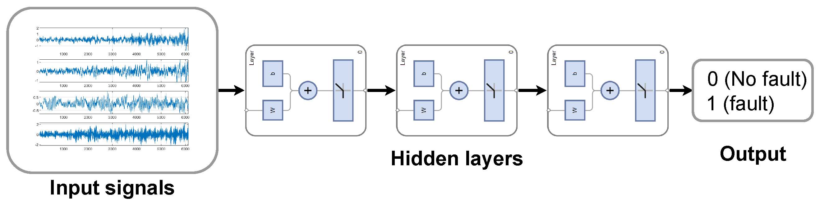There are many different types of layers; however, for the purpose of brake disc fault detection, linear layers implementing linear transformations of the input data x [12], activation functions responsible for the approximation of nonlinear behavior and convolution layers [12,38] used for automatic feature extraction were employed. Two separate neural network architectures were investigated. The first one was a so-called fully connected neural network (FCNN) containing an input, a single hidden layer and output linear layers. Each linear layer contained 10 neurons with ReLU activation functions applied on their respective outputs. A sigmoid [12] activation function was applied to the output of the last linear layer. Figure 11 illustrates the architecture of the FCNN model.

To measure the effect of automatic feature extraction, a convolutional neural network (CNN) architecture was also considered. This model consisted of a single convolution layer using one filter. That is, the layer implemented a single discrete convolution with the convolution kernel containing 40 free parameters. This was followed by a max pooling layer [15], whose output was a single value. The convolution and pooling layers are responsible for the automatic feature extraction in the model. The output of the pooling layer is passed through linear layers and nonlinear activation functions identical to the above-described FCNN (see Figure 11), which classify the extracted features. Using the same underlying fully connected architecture in the CNN model allowed for the evaluation of the effect of the convolution layer.

In addition to the above-described well-known classification schemes, some state-of-the-art classifiers used for similar problems were also considered. In particular, since the problem of lifetime estimation [39,40] is closely related to fault detection, a neural network model introduced in [39] was used. In [39], Zhang et al. proposed the use of so-called Levenberg–Maquardt backpropagation neural networks (LM-BPNNs) for the lifetime estimation of power converters. In [39], the authors argue that, for this type of task, the Levenberg–Marquardt (see, e.g., [41]) training algorithm should be preferred to the usual stochastic-gradient-method-based optimization schemes. In order to measure the effect of different training algorithms using neural network models, an LM-BPNN model was also used for brake disc detection. The network architecture matched that of the FCNN model; however, optimal model parameters were determined using the Levenberg–Marquardt algorithm. Although more complex models such as [40] might also be used to solve the problem of brake disc detection, in Section 5.2 it is shown that the investigated algorithms suffice, especially if the proposed feature transformations (i.e., Equation (4)) are also applied.

5.2. Results and Discussion

Table 2. Considered ML models and abbreviations.

Name	Abbreviation	Nonlinear Data
Support vector classifier (linear kernel)	SVM (linear)	No
Support vector classifier (radial basis kernel)	SVM (RBF)	Yes
Naive Bayes classifier	NB	Yes
Random forest classifier	RF	Yes
Fully connected neural network	FCNN	Yes
Convolutional neural network	CNN	Yes
Levenberg-Marquardt backpropagation network	LM-BPNN	Yes

summarizes the considered machine learning models for brake disc fault recognition. The table includes the abbreviations used for each model henceforth as well as an indication of whether the model is able to classify nonlinearly separable data.

The results of the five-fold cross-validation experiments using the non-overlapping dataset are given in

Table 3. Experimental results achieved using 5-fold cross-validation on the non-overlapping dataset.

Model	Feature Extraction	Avg. Acc.	Min. Acc.	Max. Acc.
SVM (linear)	-	$0.54$	$0.2$	$\mathbf{1.0}$
	PCA	$0.67$	$0.5$	$0.8$
	std	$0.9$	$0.75$	$\mathbf{1.0}$
SVM (RBF)	-	$0.54$	$0.5$	$0.6$
	PCA	$0.71$	$0.5$	$\mathbf{1.0}$
	std	$0.92$	$\mathbf{0.8}$	$\mathbf{1.0}$
NB	-	$0.58$	$0.5$	$0.8$
	PCA	$0.68$	$0.5$	$0.8$
	std	$0.85$	$0.75$	$\mathbf{1.0}$
RF	-	$0.54$	$0.25$	$0.75$
	PCA	$0.78$	$0.6$	$\mathbf{1.0}$
	std	$\mathbf{0.95}$	$0.75$	$\mathbf{1.0}$

. In the first two columns of Table 3, the name of the model and the used feature-extraction transformation are shown. The average, minimal and maximal accuracies achieved (on the test set) by each experimental setup are also displayed. The abbreviations “RF”, “SVM” and “NB” stand for random forest, support vector machine and Naive Bayes classifiers, respectively, while “std” and “PCA” indicate the use of the standard deviation (4) and PCA (5) feature-extraction transformations.

From Table 3, it is clear that each of the proposed ML classification algorithms is capable of detecting deformations on the brake disc provided that appropriate feature-extraction transformations were applied to the measurements. The difficulty of the fault-detection problem is also obvious. Without any feature-extraction steps applied, even the models capable of dealing with nonlinearly separable data (SVM using the RBF kernel and random forest classification) struggle to perform. The scarcity of data in this experiment (see Table 1) exacerbates this problem; however, the results strongly suggest that the input segments corresponding to brake disc deformations and healthy segments are not separable in a linear manner. PCA feature transformations (5) were applied to each input segment separately with only the first principal component considered; thus, using the notations in Section 4, $\mathrm{\Psi }\left(x\right)\in {\mathbb{R}}^4$ for each input segment $x\in {\mathbb{R}}^{6123\times 4}$. This parameter choice was determined by a manual search of the hyperparameter space. The application of PCA significantly increased the overall accuracy of the classification algorithms. The best average accuracy acquired using the PCA transformation, however, was only $78.0\%$, achieved by random forest classification. This would not suffice for industrial applications of the proposed measurement system. In addition, when only considering the minimal scores achieved on a single fold, PCA enhanced classification algorithms only acquired $60\%$ accuracy.

The best-performing feature-extraction scheme in this experiment turned out to be the standard-deviation-based approach (4). Applying this to the data even allowed the baseline linear classification approach (linear SVM) to achieve an average accuracy of $90\%$. In other words, the features acquired from transformation (4) are almost linearly separable. This confirms the assumption proposed in Section 4, that brake disc deformations manifest themselves as added noise on the measured acceleration signals. The best overall performance, when using the empirical standard deviation scores as features, was achieved once again by random forest classification. It is also worth pointing out that the Naive Bayes classifier consistently provided slightly worse results than the rest of the investigated models. In spite of this, the effect of the proposed feature-extraction schemes can also be observed using the NB classifier, that is, even the NB approach provides reliable and consistent results when used together with feature transformations (4).

The results from the experiments using the overlapped dataset are given in

Table 4. Experimental results achieved using the larger, overlapping dataset. In this case, more sophisticated neural-network-based models were also considered.

Model	Feature Extraction	Accuracy on Test Set
SVM (linear)	-	$0.502$
	PCA	$0.737$
	std	$\mathbf{1.0}$
SVM (RBF)	-	$0.799$
	PCA	$0.976$
	std	$\mathbf{1.0}$
NB	-	$0.655$
	PCA	$0.800$
	std	$0.854$
RF	-	$0.837$
	PCA	$0.804$
	std	$0.963$
FCNN	-	$0.573$
	PCA	$0.891$
	std	$\mathbf{1.0}$
CNN	automatic	$\mathbf{1.0}$
LM-BPNN	-	$0.599$
	PCA	$0.599$
	std	$\mathbf{1.0}$

. The abbreviations in this table match the previous notations from Table 3. Due to the abundance of data samples, the FCNN, CNN and LM-BPNN neural network models were also included in this experiment.

The results in Table 4 confirm the observations made in the non-overlapping experiments. Namely, the use of transformation (4) proved to be the most beneficial. In fact, given this larger dataset, even the baseline linear SVM classifier was able to achieve perfect accuracy on the test set using the “std” features. The rest of the two-step (feature extraction, then classification) approaches also performed similarly well, with the Naive Bayes model once again achieving the poorest result. Nonlinear classification schemes (SVM, RBF and RF) did not seem to provide a clear advantage when the “std” feature-extraction transformation was applied. The neural network models introduced in Section 5.1 also achieved an accuracy of $100\%$ for this experiment. In particular, the FCNN model behaved similarly to the other investigated ML approaches with respect to the applied feature-extraction transformation. That is, with no feature extraction applied, FCNN achieved poor results on the test set. It is important to mention that, unlike the baseline linear model, the FCNN classifier is able to differentiate between faulty and healthy acceleration signals in the training set. The poor performance on the test is a result of the FCNN model very quickly overfitting the data. When used with PCA, the FCNN’s accuracy increases significantly, while the use of the “std” feature-extraction scheme allows for perfect results on the test set. The introduced simple convolutional model (see Section 5.1) also achieves $100\%$ test accuracy. In this case, no static feature-extraction transformation was needed, as the convolution layer in the model acted as an adaptive feature transformation.

Finally, the state-of-the-art LM-BPNN method was investigated. The application of the Levenberg–Marquardt optimization scheme yielded similar results to the FCNN. It is observed that the performance of the neural-network-based models seemed to depend less on the employed training method and more on the representation of the input signals by choosing the correct feature transformation. Similarly to the other investigated models, the LM-BPNN performed best when used together with the feature transformation given in Equation (4). With this feature-extraction step, LM-BPNN could achieve perfect accuracy on the test set.

Overall the results in Table 3 and Table 4 prove that the proposed measurement system used with ML methods is capable of detecting brake disc deformations. Furthermore, it is possible to conclude that low-complexity algorithms (RF and linear SVM) may be used to efficiently solve the investigated fault-detection problem provided the measurements are transformed according to (4). In fact, the accuracy of these classifiers matches the performance of a much more complex convolution-based neural network. For real-time brake disc fault detection, the use of static feature extraction together with a simpler but more interpretable model (such as linear SVM) is preferable, because the model parameters contain meaningful information to humans. Another advantage of the simpler models from the point of view of industrial applications is that these algorithms have previously been efficiently implemented on low-cost hardware such as microcontrollers (see, e.g., [17,18]). Using the findings presented in this paper, constructing a measurement system where brake disc fault detection is conducted real time is a promising pursuit. It is worth pointing out that the CNN architecture used in this study is also small enough to be implemented on low-cost hardware. In order to support reproducible research, the codes and measurement data used to generate the above results have been made publicly available and can be accessed at [42].

6. Conclusions

In this study, a novel measurement system for brake disc fault detection was proposed. The measurement system consisted of two parts: a physical realization using four acceleration sensors attached to the test vehicle and a software-based signal-processing component. Because of the nonlinear and non-stationary nature of the measurements, in the latter component, a number of ML-based algorithms were investigated. In addition to the use of ML, intuitive feature-extraction schemes were utilized which provided more interpretable models with simpler architectures. Measurements corresponding to a real-life emergency braking scenario were conducted on a test track. With the help of these measurements, the effectiveness of various signal-processing methods was compared. It was discovered that an intuitive empirical-deviation-based feature-extraction scheme together with a geometrically interpretable linear support vector machine classifier allowed for precise fault detection. Since the parameters of linear SVMs retain geometrical meaning [29], it is the conclusion of this study that light-weight architecture, partially interpretable ML models are sufficient to construct the signal-processing part of the proposed measurement system. In this paper, the proof of concept for the effectiveness of the proposed measurement system was provided. Several problems can be considered in the next phase of this research. For example, the hardware part of the measurement system could be enhanced with wheel angle measuring apparatus. This would remove the need for the signal-segmentation scheme discussed in Section 3. In addition, the hardware-based segmentation of the measurements to single wheel revolutions would allow the use of time–frequency-based signal representations such as Gabor or wavelet transformations [23].

In this study, a simple test scenario of the vehicle accelerating along a straight trajectory then performing emergency braking was investigated. For real-life use of this technology, however, further experimentation is necessary. For example, in the next phase of this research, experiments where the vehicle moves along a more diverse trajectory and performs a variety of less intensive braking maneuvers will be conducted. Increasing the complexity of the test scenarios will likely require more sophisticated signal-processing ML algorithms as well. For example, in order to retain the interpretable nature of well-performing models in these cases, so-called model-driven classifiers will be investigated [17,25,43]. These ML models aim to incorporate analytic mathematical transformations into ML methods in a way such that the optimized parameters retain physical meaning. Model-driven architectures have successfully been used to solve several problems related to vehicle control such as road quality estimation [28], fault detection of accelerometer sensors [17] and bearing fault detection [43].