Essay

Research on the Remaining Life Prediction Method of Rolling Bearings Based on Optimized TPA-LSTM

Mechanical Science and Engineering Institute, Northeast Petroleum University, Daqing 163318, China
*
Author to whom correspondence should be addressed.
Machines 2024, 12(4), 224; https://doi.org/10.3390/machines12040224
Submission received: 1 March 2024 / Revised: 21 March 2024 / Accepted: 26 March 2024 / Published: 27 March 2024
(This article belongs to the Section Machines Testing and Maintenance)

Abstract

:
The whole life cycle degradation data set of rolling bearings has the characteristics of large capacity, diversity, and non-stationarity. As a powerful tool for processing such time series data in deep learning algorithms, LSTM is prone to the loss of important time series information in the process of the life prediction of rolling bearings, which leads to a decline in prediction accuracy. Therefore, a method for predicting the remaining useful life (RUL) of rolling bearings based on the combination of temporal pattern attention mechanism (TPA) and LSTM is proposed. The method firstly combines hierarchical clustering and principal component analysis (PCA) to construct a multi-faceted and multi-scale preferred feature set reflecting the degradation information of rolling bearings, then strengthens the information correlation between hidden layers of the LSTM model through TPA and optimates the parameters of the fusion model of TPA and LSTM by using the gazelle optimization algorithm (GOA). Finally, the model is applied to the experimental data set of rolling bearing degradation. The results show that, compared with the traditional model, this method is more suitable for the remaining life prediction of rolling bearings.

1. Introduction

In recent years, the rapid development of high-end heavy equipment such as high-speed rail, turbines, and industrial robots has placed higher and higher requirements on the reliability and safety of equipment. Data show that about 45% to 55% of mechanical failures in rotating machinery are caused by rolling bearing failure [1]. As a key component of high-end heavy equipment, rolling bearings usually operate under high-speed, heavy-load conditions and are extremely susceptible to wear and tear, which can cause equipment failure, serious economic losses, and even casualties. Therefore, it is crucial to choose an appropriate method, make full use of real-time monitoring data from rolling bearings, accurately predict the RUL of rolling bearings, and provide a reliable basis for predictive maintenance of equipment.
At present, rolling bearing RUL prediction methods are mainly divided into two types: one is based on the failure mechanism model and the other is data-driven. The prediction method based on the fault mechanism model refers to constructing a failure physical model that reflects the rules between the rolling bearing fault state and system parameters through theoretical derivation or large-scale experimental analysis [2]. However, bearing failures in equipment such as aerospace engines and industrial robots are characterized by multi-factor coupling and complex transmission paths, which often require the establishment of extremely complex mechanical models, making it difficult to obtain accurate results. Relying on abundant measured data throughout the life cycle of rolling bearings, the data-driven prediction method does not require in-depth study of the coupling of multiple failure factors in the external environment of the bearing and the complex degradation mechanism inside the bearing. Therefore, this method has received widespread attention from scholars. Data-driven prediction methods can be divided into statistical models and machine learning. The prediction method based on the statistical model first establishes a random degradation model of the rolling bearing and estimates and updates the unknown parameters of the model through a large number of historical performance degradation data and field data of the same operating condition and the same model of rolling bearings, thereby obtaining the RUL expression of the rolling bearing in the form of a probability distribution. At present, significant progress has been made in the prediction methods based on statistical models. Scholars have successively proposed rolling bearing degradation modeling under different situations such as multiple uncertainties [3], nonlinearity [4], multi-stage [5], and multi-source information fusion [6]. Although complex stochastic degradation models can effectively track and predict the degradation trend of rolling bearings, they need to assume more unknown parameters, making the model parameters more difficult to estimate. The accuracy of prediction methods based on statistical models greatly depends on the accurate estimation of model parameters. At the same time, rolling bearing degradation data are affected by multiple working conditions and models and the degradation process is random and variable. Therefore, the accuracy of the method for predicting rolling bearing RUL based on statistical models needs to be improved.
The prediction method based on machine learning generally consists of four technical processes, namely data collection, health indicator (HI) construction, health stage (HS) division, and RUL prediction [7]. The construction of a high-quality HI is the prerequisite for high-precision RUL prediction. The monitoring data collected through sensors has the characteristics of large capacity, nonlinearity, and non-stationarity. How to mine useful information from the huge data is the key to bearing RUL prediction. A large amount of random noise mixed in with the monitoring data increases the difficulty of constructing an HI. Tang et al. [8] proposed a noise reduction method based on the fusion of local mean decomposition (LMD) and multi-scale entropy (MSE). This method first uses LMD to decompose the original signal into multiple components that are then filtered out with a low signal-to-noise ratio through mutual information values; finally, the MSE composition feature set of the remaining components is obtained. Experiments show that this method has extremely strong noise reduction capabilities. Wang et al. [9] used variational mode decomposition (VMD) to decompose the original signal into global degradation components and local fluctuation components. This method classifies noise and random fluctuations into one category, making full use of the characteristic information of the original signal. As an effective indicator of the physical quantities reflecting the degradation of rolling bearings, RMS is widely used because of its good interpretability and monotonicity [10]. However, often a single feature can only reflect the single-scale feature information of the time series and the analysis effect has certain limitations. Therefore, many scholars extract rolling bearing degradation characteristics from different perspectives such as the time domain, frequency domain, and time–frequency domain to form feature sets [11]. Zhang et al. [12] screened the feature set based on the weighted sum of three indicators, monotonicity, correlation, and robustness, and extracted the optimal features. It is important to construct an HI that can map the degradation trend of rolling bearings. Principal component analysis (PCA) can fuse high-dimensional feature sets into low-dimensional feature curves as bearing HIs without losing much feature information and is an important means to deal with this type of problem [13].
Reasonable division of health stages and determination of rolling bearing degradation starting points and failure points are of great significance to rolling bearing RUL prediction and subsequent maintenance strategies. Mao et al. [14] first found the maximum slope point of the singular value decomposition (SVD) normalized correlation coefficient, then found the point at the same time on the RMS as the individual bearing change point, and finally averaged all individual bearing change points as the starting point of bearing degradation. starting point. Li et al. [15] determined the 3σ interval by calculating the average and standard deviation of kurtosis and considered the exceeding 3σ interval as an abnormal state of the rolling bearing. Jin et al. [16] used Box–Cox transformation and Gaussian distribution to determine the starting point of degradation and divided the degradation stage of rolling bearings into a health stage and a wear stage. In summary, based on the threshold method, the starting point of rolling bearing degradation can be objectively determined. However, due to the weak fault information of rolling bearings in the early degradation stage, there is a situation where the segmentation points of the healthy stage and the degradation stage are extremely blurred. At the same time, due to the uncertainty of individual differences in rolling bearings, the degradation trend of some rolling bearings is poor in monotonicity, which can easily lead to misjudgment of the starting point of degradation. Therefore, how to accurately find the starting point and failure point of rolling bearing degradation while ensuring the objectivity of the classification basis requires further research.
Machine learning has powerful feature extraction capabilities and is widely used in speech translation, image recognition, fault diagnosis, RUL prediction, and other fields. Wang et al. [17] combined the BP neural network with the ARIMA model and applied it to fan RUL prediction. Experimental results show that this method can make up for the shortcomings of the large prediction errors of a single BP neural network. Zhang et al. [18] used a genetic algorithm (GA) to optimize the BP neural network to achieve RUL prediction for cutting tools. Experimental results show that this method can also improve the accuracy of model prediction. However, a BP neural network also has the disadvantages of slow convergence speed and ease of falling into local minimization. Chen et al. [19] proposed an improved hybrid model RUL prediction method that combines the multivariate gray model (MVG) and the radial basis neural network (RBF). This method can solve the problems of a small number of prediction samples, insufficient sequence integrity, and local minimization and has the advantages of a simple structure and fast convergence speed; however, this method is only suitable for short- and medium-term and exponential growth predictions. Wang et al. [20] proposed an online sequential extreme learning machine (OS-ELMK) with a kernel to solve the non-stationary problem of time series. Miao et al. [21] applied a support vector machine (SVM) to gyroscope RUL prediction. They first used wavelet decomposition to weaken the influence of random items in time series and highlight the trend items and then introduced a GA-optimized SVM for time series prediction. This method shows that the SVM has strong generalization processing capabilities. However, for long-term time series prediction, the SVM has problems such as a long training cycle and high risk of overfitting. To sum up, traditional machine learning mostly adopts shallow model design and cannot represent the complex mapping relationships of time series.
In today’s big data context, rolling bearing monitoring data mostly exhibits nonlinear, diverse, and multi-dimensional characteristics. Among various machine learning algorithms, deep learning algorithms have powerful feature learning capabilities, nonlinear fitting capabilities, flexible model structure expansion capabilities, and can better handle diversified rolling bearing performance degradation data. Therefore, they are widely used in the field of rolling bearing RUL prediction. They have developed rapidly, and a large number of deep neural networks have been developed and applied to rolling bearing RUL prediction. Babu et al. [22] used a convolutional neural network as a rolling bearing RUL prediction model, and their results show that the prediction accuracy of this method is better than traditional machine learning. Zhu et al. [23] applied a multi-scale convolutional neural network (MSCNN) to rolling bearing RUL prediction. Compared with a traditional CNN, the MSCNN can learn global information and local information simultaneously, improving the model prediction accuracy and stability. Li et al. [24] used a CNN to extract the multi-scale features of vibration data for equipment RUL prediction. This method shows that the CNN can replace traditional signal processing and remove manual experience to achieve an end-to-end prediction method, making RUL prediction more intelligent. The above shows that increasing the depth and complexity of the CNN model can enhance the learning ability of the CNN, but excessively increasing the depth of the model will increase the time cost of model prediction and, at the same time, network degradation problems will occur. In this regard, Mo et al. [25] added the residual network (ResNet) to a CNN for device RUL prediction, which solved the problems of gradient disappearance, gradient explosion, and network degradation that occur with the superposition of convolutional layers and pooling layers and accelerated the model convergence.
Rolling bearing monitoring data contain a large amount of timing information. Although CNNs have powerful high-dimensional feature extraction capabilities, they do not have the memory function of time series information. The recurrent neural network (RNN), as a deep learning network that specializes in processing time series data, has proven its power in application fields such as natural language processing (NLP), speech recognition, and web resource recommendation. Inspired by this, Heimes [26] applied an RNN to equipment RUL prediction and proved on the NASA data set that the RNN’s ability to predict time series is stronger than other neural networks. Guo et al. [27] used an RNN to extract rolling bearing degradation data to construct an HI. The results showed that the HI constructed by this method has high monotonicity and correlation, proving that RNNs can also replace traditional signal processing. Wang et al. [28] proposed an RUL prediction method based on a cyclic convolutional network (RCNN) and applied it to rolling bearing and milling cutter data sets. The results show that this method has high accuracy and convergence. Although RNNs have the memory function of time series data, when RNNs handle long time series prediction problems, they will also expose two major drawbacks: gradient disappearance and gradient explosion. LSTM and a gated recurrent unit (GRU) were proposed to solve this type of problem. Wang et al. [11] applied LSTM to rolling bearing RUL prediction, and their results showed that LSTM has high accuracy in long time series prediction. Huang et al. [29] used a bidirectional long short-term memory network (BiLSTM) to perform feature extraction and RUL prediction on turbofan engine data. The results show that this method has higher generalization performance compared to LSTM. In order to fully mine high-dimensional features, Meng et al. [30] superimposed multiple deep convolutional long short-term memory networks (CLSTMs) layer by layer to predict device RUL. Bai et al. [31] proposed a new time series prediction model, the temporal convolution network (TCN), by changing the architecture of a CNN. The results show that the TCN is superior to the traditional LSTM in extracting temporal features, and it also has the ability of time memory. However, due to the limited receptive field, this model can only capture the local degradation features of rolling bearings with a fixed length and cannot effectively deal with the global dependency relationship of degradation features of rolling bearings like LSTM.
The quantification of uncertainty in predicting the remaining life of rolling bearings has important application value for subsequent maintenance decisions. She et al. [32] added a bootstrap algorithm to the prediction model to quantify the prediction uncertainty and found that this algorithm can flexibly and intuitively evaluate the reliability without prior knowledge and sensitively capture the prediction error caused by data changes. Jiang et al. [33] combined the prediction model with a Bayesian neural network (BNN) to quantify the prediction uncertainty of rolling bearing RUL and realized the complementary advantages of the network. These methods have shown considerable prospects in application, but there are still some unresolved issues. When processing large-scale data, its computational time cost limits its practical feasibility. Furthermore, the robustness of the BNN will be constrained by prior distribution selection.
This paper improves the RUL prediction method of rolling bearings based on LSTM based on the research of scholars. In actual engineering service, there is often a long time span from the initial degradation to the failure of rolling bearings. Although LSTM can effectively handle the long-term dependence of rolling bearing degradation characteristics, its ability is not sufficient to cope with practical applications. Therefore, the long-term memory ability of LSTM still needs to be improved. The accurate setting of the LSTM model parameters is very important for its prediction accuracy, but manual adjustment of parameters will greatly increase time cost and workload. At the same time, the commonly used methods to quantify the uncertainty have adaptability problems.
In order to overcome the above problems, this paper proposes a rolling bearing RUL prediction method based on GOA-TPA-LSTM. The major contributions of this work are: (1) using an LSTM model with added TPA for RUL prediction of rolling bearings to enhance LSTM’s memory ability; (2) selecting the GOA algorithm to optimize the parameters of the prediction model, reducing the time cost and workload of manually adjusting parameters; and (3) the combination of quantile regression and prediction models for the interval probability prediction of rolling bearings has achieved complementary advantages of the models.
The remainder of the paper is organized as follows: In Section 2, we introduce the basic theories of LSTM and the TPA and GOA and established an RUL prediction framework for rolling bearings based on these three methods. In Section 3, we apply this framework to the accelerated life test data of rolling bearings. Conclusions are drawn in Section 4.

2. Theoretical Analysis of the Rolling Bearing RUL Prediction Model

Rolling bearings of different operating conditions and models show significant differences in degradation trends. At the same time, the degradation characteristics of rolling bearings have long-term correlation globally and show nonlinearity and fluctuation enhancement locally. Long-term correlation refers to the numerical correlation of rolling bearing degradation data over a long period of time; nonlinearity and fluctuation enhancement means that the local change trend is disordered, and the degree of fluctuation increases as time goes by. These characteristics greatly increase the prediction difficulty of the model. To solve this problem, this paper chooses to use LSTM to predict the RUL of rolling bearings. In order to enhance the model’s ability to recognize and remember key timing features, the TPA mechanism is introduced. In order to make the model suitable for the RUL prediction of rolling bearings of different working conditions and different models, GOA is added to adaptively optimize the model parameters. The following is a focused introduction to the model.

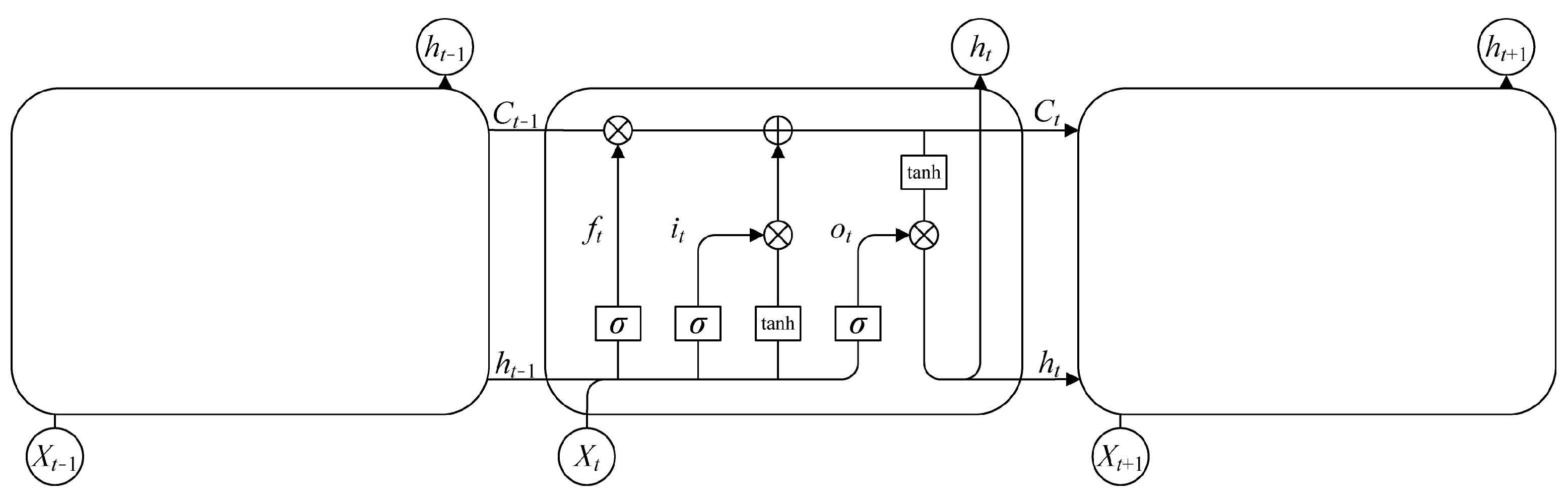
2.1. Basic Theory of LSTM

LSTM was proposed to solve the long-term dependency problem of RNNs. That is, when modeling time series, after several iterative calculations, earlier time series features will be overwritten by new features, resulting in new features. The information contained is reduced, so that the model loses its ability to learn long-term information [11]. In order to solve the long-term dependency problem, LSTM introduces the concept of gating, which controls the circulation and loss of features through multiple gates. Its unit structure is shown in Figure 1.
Forgetting gate: The forgetting gate determines the degree of retention of state information at the previous moment. The calculation formula is:
f t = σ ( W f h t 1 + U f x t + b f )
Input gate: The input gate determines whether the status of the unit is updated. The calculation formula is:
i t = σ ( W i h t 1 + U i x t + b i )
a t = tanh ( W a h t 1 + U a x t + b a )
C t = f t C t 1 + i t a t
Output gate: The output gate determines the final output value of the unit. The calculation formula is:
o t = σ ( W o h t 1 + U o x t + b o )
h t = o t tanh ( C t )
where W and U are the weight coefficients; b is the bias coefficient; σ is the sigmoid activation function; tanh is the tanh activation function; xt is the input at time t; ht is the hidden state at time t; and Ct is the internal state at time t.

2.2. Basic Theory of TPA Mechanism

In order to obtain the importance of inputs at different moments to the predicted value, TPA first uses multiple one-dimensional convolution kernels to extract the time series features of fixed length from hidden state ht output by LSTM, then the weights of the current time ht and the previous time ht-w are determined by the scoring function and the final hidden state ht is obtained according to the weights of the current time [34]. The LSTM adding TPA focuses on the correlation between the hidden layer output value at different times in the past and the hidden layer output value at the current moment, which enhances the sensitivity of the input value at key historical moments and thereby enhances the prediction model’s ability to recognize and remember key temporal features. The block diagram of the TPA mechanism is shown in Figure 2.
The calculation formula is:
CNN extracts the temporal feature matrix H i , j C :
H i , j C = i = 1 w H i , t w 1 + l C j , T w + l
Calculate the temporal pattern weight vector vt:
f ( H i C , h t ) = ( H i C ) T W a h t
α i = σ ( f ( H i C , h t ) )
v t = i = 1 m α i H i C
Calculate the hidden state at the current moment h t :
h t   =   W h ( W h h t + W v v t )
where H i , t w 1 + l = [ h t w , h t w + 1 , , h t 1 ] , w is the length of the time series of interest, represents convolution operation; C j , T w + l is the convolution kernel, T represents the convolution kernel size; and W i , h , h , v is the weight matrix.

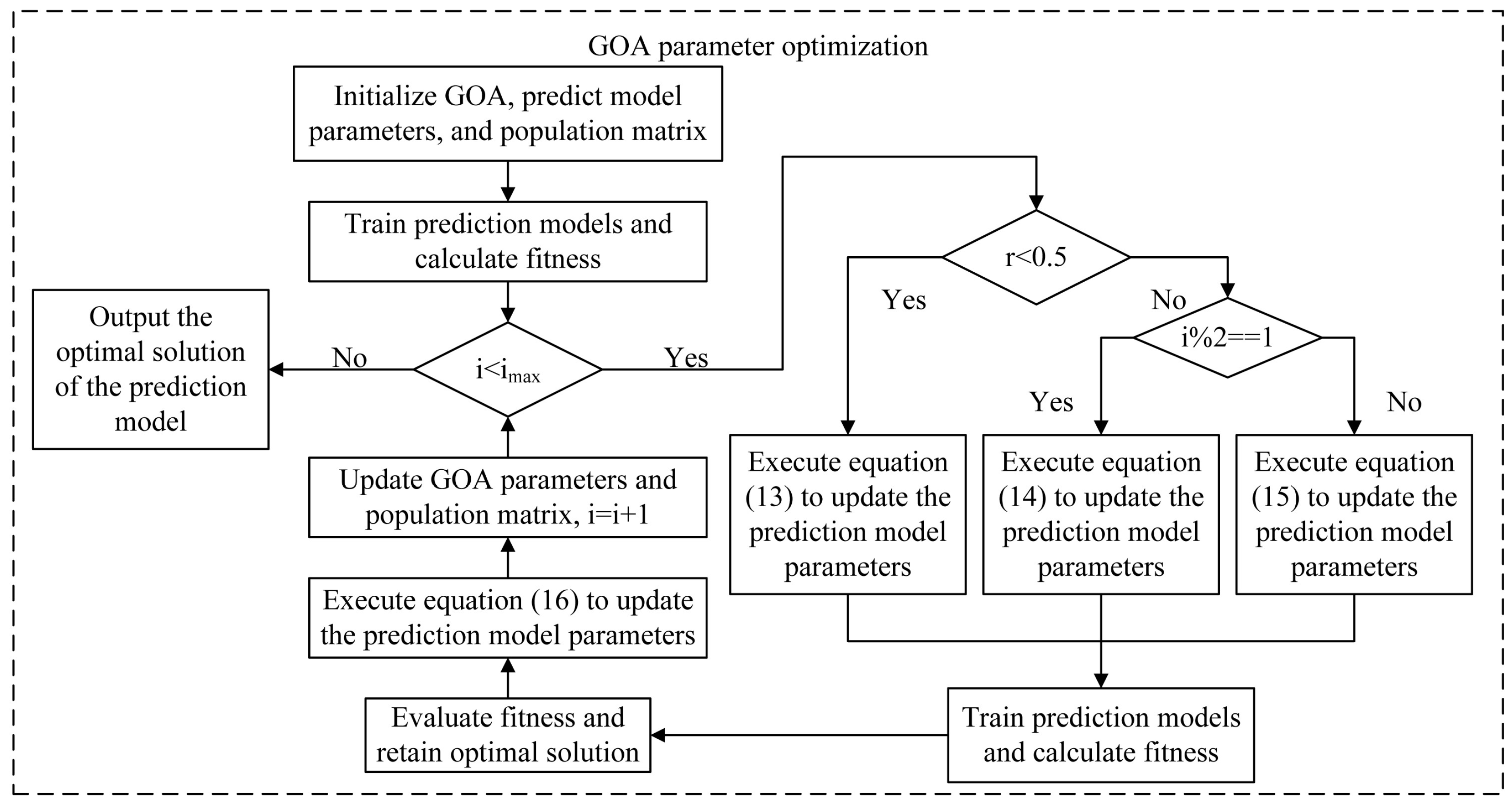
2.3. Basic Theory of GOA Algorithm

The GOA algorithm is a new global intelligent optimization algorithm proposed by Agushaka et al. [35] that was inspired by the behavior of gazelles escaping predators. It has powerful optimization efficiency and convergence functions. In this paper, the algorithm is used to find the optimal hyperparameters of the prediction model. The basic modeling steps of the GOA are as follows:
(1)
Random initialization of the population
X = x 1 , 1 x 1 , 2 x 1 , d x 2 , 1 x 2 , 2 x 2 , d x n , 1 x n , 2 x n , d
where n represents the number of populations; d represents the dimension of the problem to be optimized; x i , j = r · ( U j L j ) + L j ; r is a random number between [0, 1]; and Uj and Lj are the upper and lower bounds of the parameters to be optimized, respectively.
(2)
Global search
y i + 1 = y i + v · R · R B · ( X i R B · y i )
where y i + 1 is the solution of the i + 1 iteration; y i is the solution of the i iteration; v represents the individual’s moving speed; R is a vector composed of random numbers between [0, 1]; and R B is a random number vector of Brownian motion.
(3)
Local search
When the number of iterations is an odd number, the first stage is taken.
y i + 1 = y i + v · μ · R · R L · ( X i R L · y i )
where μ is −1 or 1 and R L is a random number vector from L e v y distribution. That is, L e v y ( α ) = 0.05 · a · b 1 α , a = N ( 0 , σ a 2 ) , α = 1.5 , b = N ( 0 , σ b 2 ) , σ a = Γ ( 1 + α ) sin ( π α / 2 ) Γ ( ( 1 + α ) / 2 ) α 2 ( α 1 ) 2 1 α , σ b = 1 .
When the number of iterations is an even number, the second stage is taken.
y i + 1 = y i + v · μ · C F · R B · ( X i R L · y i )
where C F = ( 1 i / i max ) ( 2 i i max ) represents the cumulative effect of predators.
(4)
Gazelle escape
y i + 1 = y i + C F [ L + R · ( U L ) ] · d y i + [ 0.34 · ( 1 r ) + r ] ( y r 1 y r 2 ) r 0.34 r > 0.34
where d = 0 1 r < 0.34 r = 0.34 and r1 and r2 are random integers between [imin, imax].
The optimization flow chart of the GOA algorithm is shown in Figure 3.

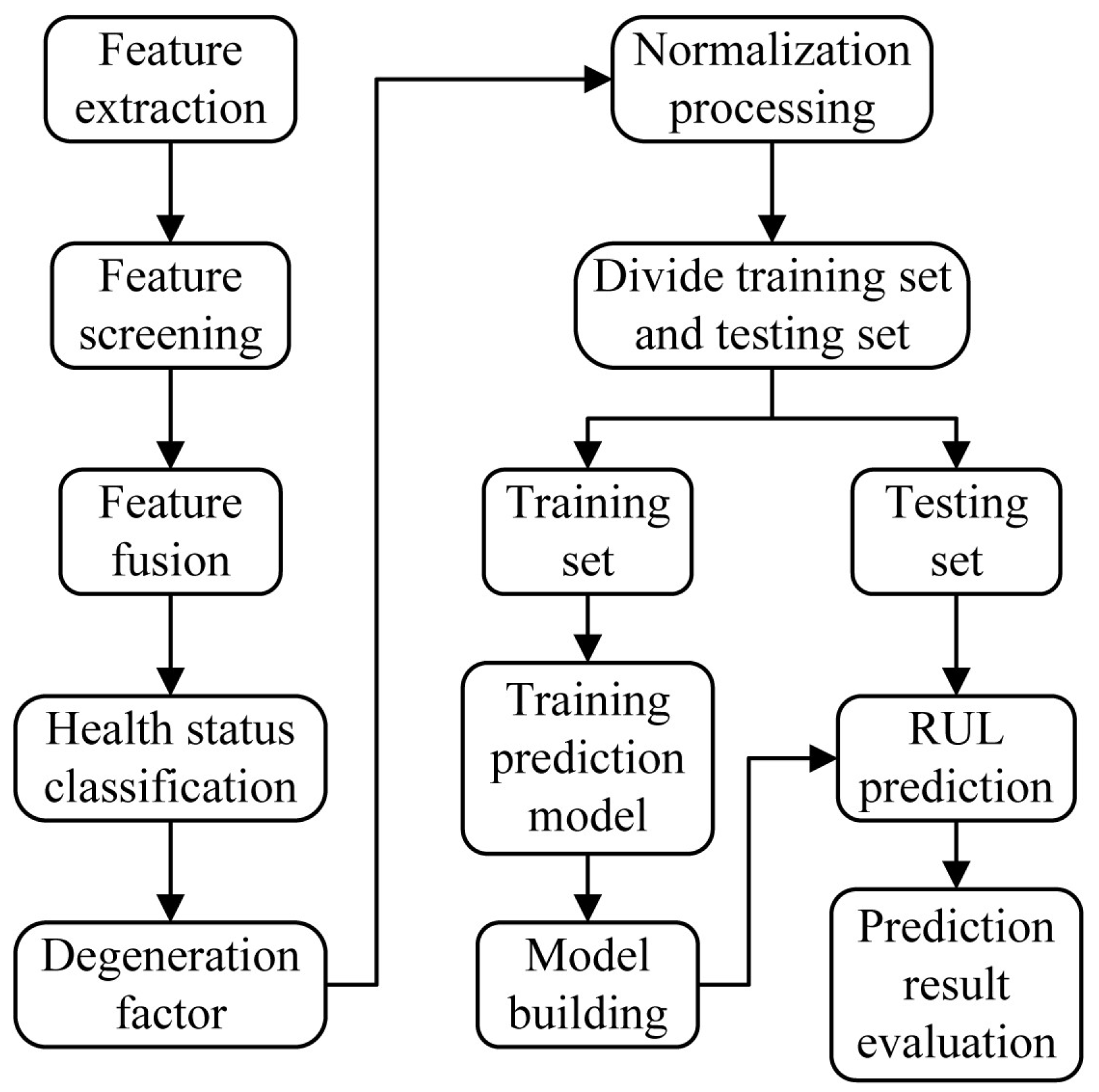
2.4. RUL Prediction of Rolling Bearing Based on GOA-TPA-LSTM

The technical route of the prediction method of rolling bearing RUL based on the GOA-TPA-LSTM model proposed in this paper is shown in Figure 4, and the specific steps are as follows:
(1)
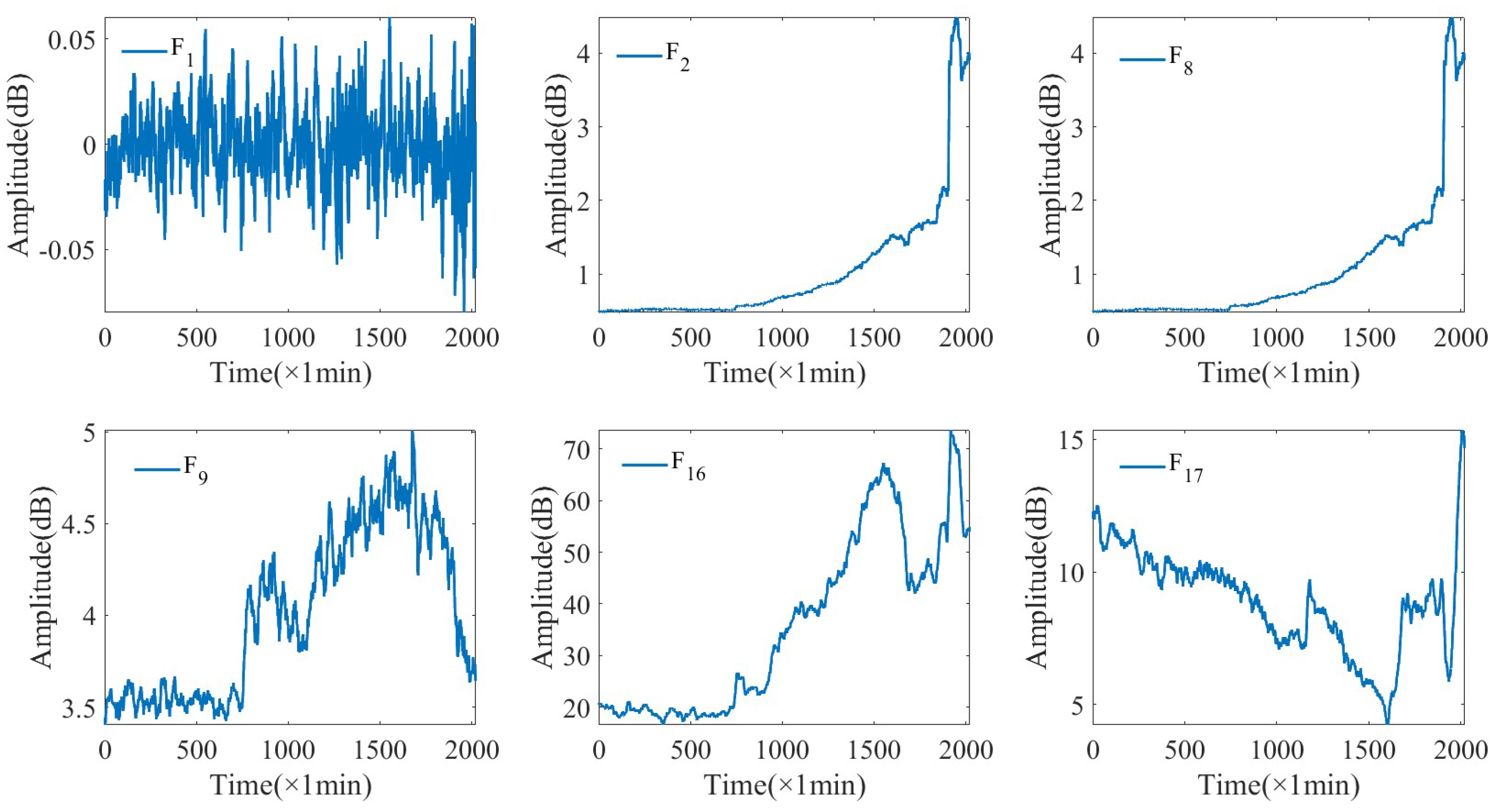
Extracting the degradation feature of rolling bearings from time domain, frequency domain, and time–frequency domain to build a feature set;
(2)
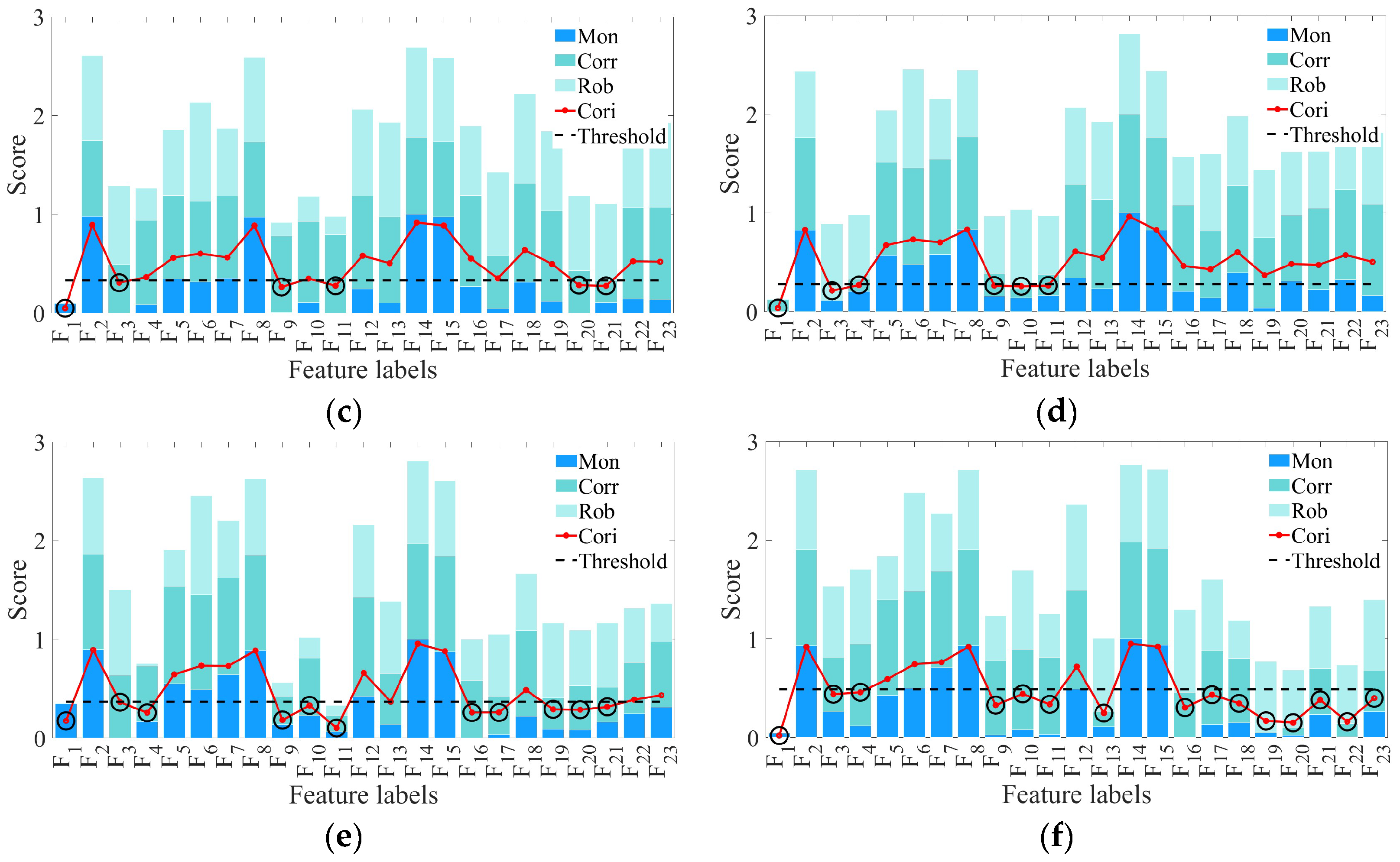
Screening feature sets based on monotonicity, time series correlation, and robustness;
(3)
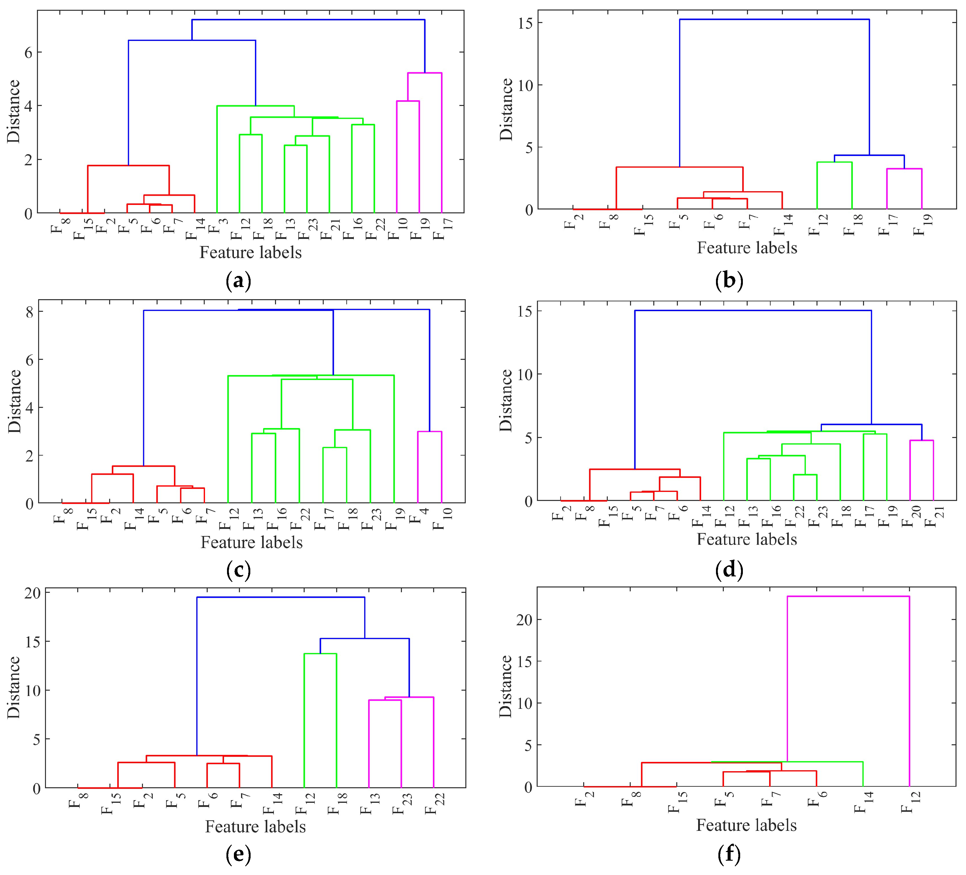
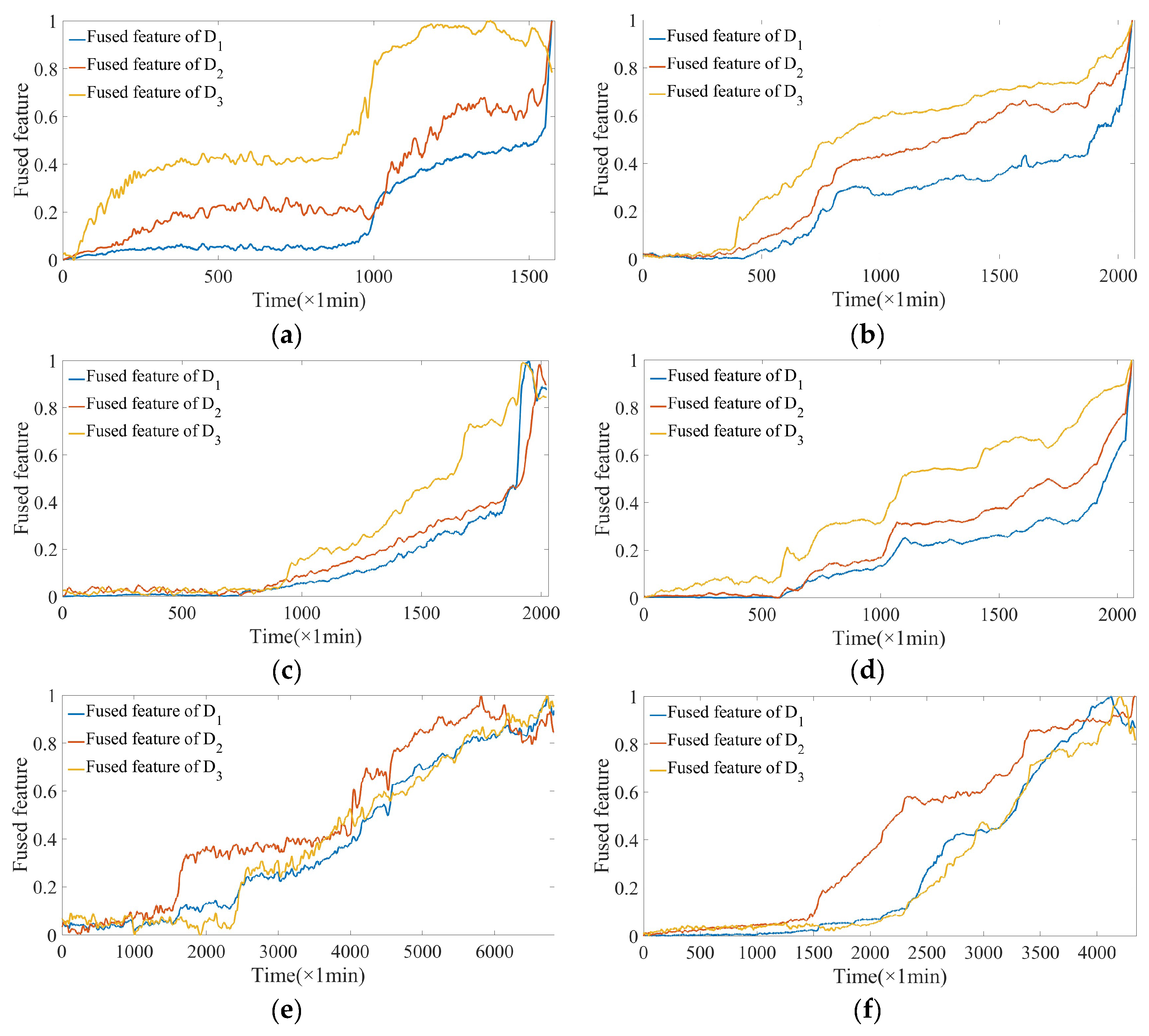
Combining hierarchical clustering and PCA to fuse feature sets;
(4)
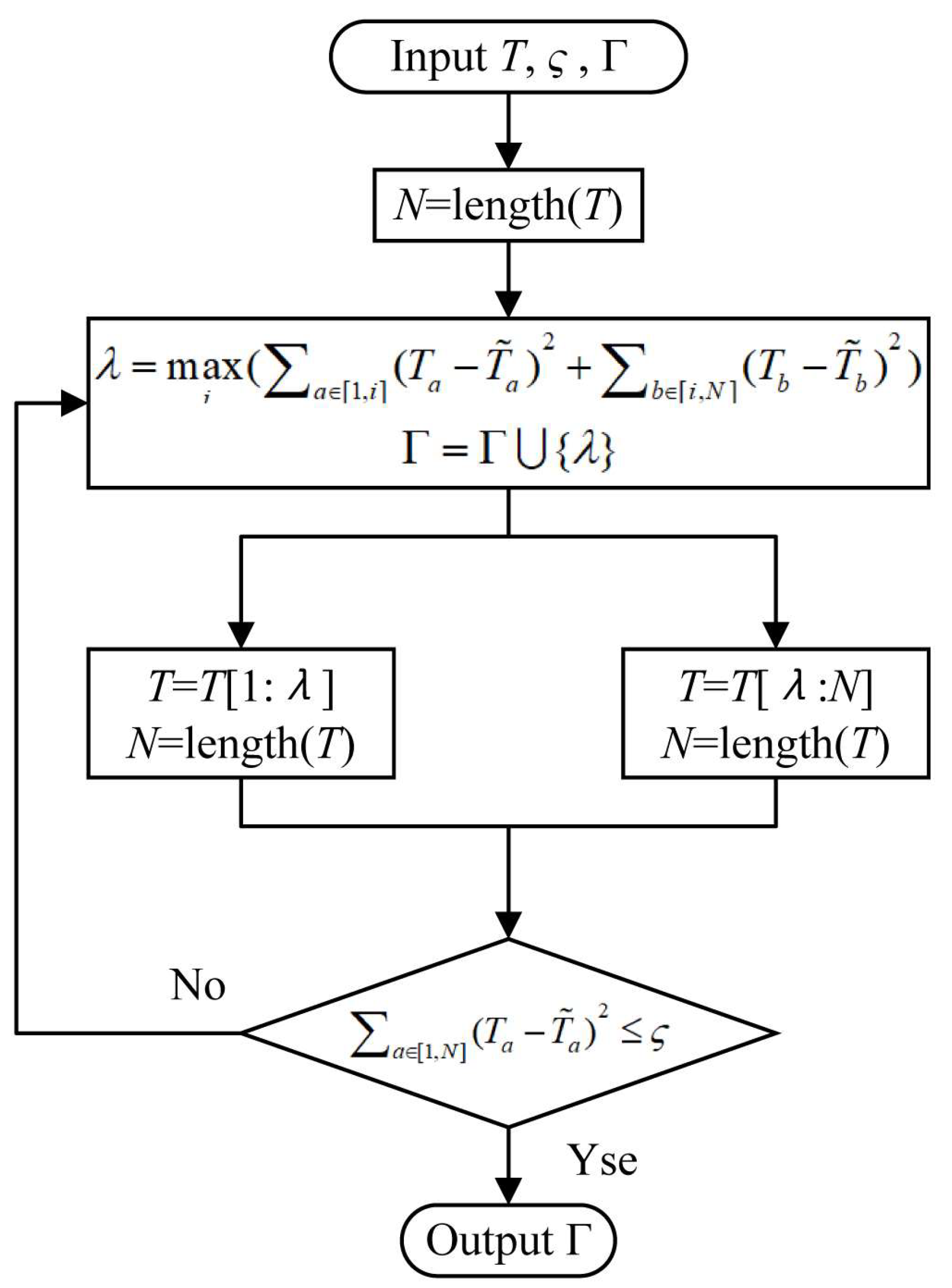
Using the top-down (TPD) algorithm to divide the fused features into health stage, degradation stage, and failure stage, and using the features of the degradation stage as degradation factors for subsequent prediction;
(5)
Normalize the degradation factor and divide the dataset into training and testing sets;
(6)
Using TPA-LSTM as the prediction model and optimizing its parameters through GOA, the training set is used as input to train the model;
(7)
Input the testing set into the trained prediction model for RUL prediction;
(8)
Evaluate the prediction results and verify the effectiveness of the method proposed in this paper.

3. Experimental Study

3.1. Introduction to Data Sets

The vibration signal data comes from the XJTU-SY rolling bearing accelerated life test data set [36]. The data acquisition test bench is shown in Figure 5. The test bearing in this data set is an LDK UER204 rolling bearing. Two unidirectional acceleration sensors measure the transverse and longitudinal vibration signals. The sampling frequency is set to 25.6 kHz, the sampling interval is 1 min, and the duration of each sampling is 1.28 s. This data set includes full-life vibration acceleration data of a total of 15 bearings under three working conditions. The test condition design is shown in Table 1. Since the vibration signal in the horizontal direction contains more useful information [37], this paper selects Bearing 1_1, Bearing 1_2, and Bearing 1_3 under the first horizontal working condition of the bearing and Bearing 2_2, Bearing 2_3, and Bearing 2_5 under the second working condition as the research objects, recorded as C1~C6.

3.2. Rolling Bearing HI Construction

3.2.1. Feature Extraction

In order to quantify the degradation trend of rolling bearings in multiple aspects and at multiple scales, 12 time domain features are first extracted (average, standard deviation, skewness, kurtosis, maximum value, minimum value, peak-to-peak value, root mean square, amplitude factor, waveform factor, impact factor, and margin factor), alongside three frequency domain features (center of gravity frequency domain, average frequency domain, and frequency domain root mean square) and eight wavelet packet node energies. A total of 23 features are used to construct the feature set, recorded as F1~F23. Then, the outliers of the 23 features in the feature set are eliminated. At the same time, in order to weaken the impact of short-term random fluctuations and noise on features and highlight the long-term trends of features, the moving average (MA) was performed on 23 features in the rolling bearing feature data set, and the sliding window was set to 30. Finally, the feature set was normalized. Figure 6 shows the partial feature curves of the feature set after bearing C3 processing.

3.2.2. Screening of Rolling Bearing Feature Sets

There are features in the feature set that cannot represent the degradation trend of rolling bearings and are severely contaminated by noise. This paper selects a comprehensive index consisting of monotonicity, temporal correlation, and robustness to screen the original feature set. Among them, the higher the monotonicity, the greater the trend that the feature value continues to increase or decrease over time; the higher the time series correlation, the stronger the correlation between the feature sequence and the time series; and the higher the robustness, the feature sequence is resistant to anomalies and the higher the tolerance of the value. The definitions of the three are as follows:
M o n ( f i ) = # d / d f i > 0 N 1 # d / d f i < 0 N 1
C o r r ( f i , T i ) = i = 1 N ( ( f i f ¯ ) ( T i T ¯ ) ) i = 1 N ( f i f ¯ ) 2 i = 1 N ( T i T ¯ ) 2
R o b i ( f i ) = ( i = 1 n exp ( r e s f i f i ) N )
where # d / d f i > 0 represents the number of eigenvalues whose derivative is greater than 0, # d / d f i < 0 represents the number of eigenvalues with derivatives less than 0; N represents the total number of eigenvalues; fi represents the feature sequence; and Ti represents the time series. r e s f i = f i s m o o t h e d _ f , process fi as a moving average to obtain smoothed_f.
When calculating the comprehensive index, first normalize fi and Ti to [0, 1]. When Ti is 0, it means the monitoring start time, and when Ti is 1, it means the rolling bearing failure time. Then, the monotonicity, temporal correlation, and robustness of the 23 features were obtained. Since the three performance indicators are all relative quantities, the three indicator values must first be scaled to [0, 1] according to the maximum–minimum value and then the comprehensive indicator can be obtained. This paper selects the weighted average of three performance indicators as the comprehensive indicator, and the weights are 0.5, 0.3, and 0.2, respectively. Finally, features whose comprehensive index is less than the threshold are filtered out to obtain the optimal feature set.
The three indicators of robustness, time correlation, and robustness and the comprehensive indicator of the 23 features in the bearing C1~C6 feature set were obtained. The screening threshold is determined by the 3σ criterion. Figure 7 shows the three screening indicators and comprehensive indicator results of the 23 features in the bearing C1~C6 feature set.
It can be seen from Figure 7 that by calculating the comprehensive index of each feature of the four bearing feature sets, the features screened out for bearing C1 are F1, F4, F9, F11, and F20; the features screened out for bearing C2 are F1, F3, F4, F9, F10, F11, F13, F16, F20, F21, F22, and F23; the filtered out features of bearing C3 are F1, F3, F9, F11, F20, and F21; the screened out features of bearing C4 are F1, F3, F4, F9, F10, and F11; the filtered out features of bearing C5 are F1, F3, F4, F9, F10, F11, F16, F17, F19, F20, and F21; and the screened out features of bearing C6 are F1, F3, F4, F9, F10, F11, F13, F16, F17, F18, F19, F20, F21, F22, and F23.

3.2.3. Construction of a Rolling Bearing HI Based on Hierarchical Clustering and PCA Fusion

There are also a large number of redundant features in the selected feature set, which will increase the time cost of the prediction process and the complexity of the prediction model, increase the risk of overfitting the model, and reduce the generalization ability of the model. This paper uses the method of clustering first and then fusion to eliminate the impact of redundant features on subsequent predictions. First, the feature set is divided into three clusters through hierarchical clustering based on the similarity between the features of the feature set, and the similarity evaluation index is the Euclidean distance; then, PCA feature fusion is performed on all features in each cluster and a total of three fusion features are obtained. Finally, the optimal feature among the three fused features is selected as the HI that reflects the degradation trend of the rolling bearing. Since the full life cycle of a rolling bearing includes a healthy stage, a mild degradation stage, an accelerated degradation stage, and a failure stage, the ideal rolling bearing HI should be a steady-rising-accelerating rise-abnormal trend. The average height is selected as the evaluation index, and the formula is a v h = i = 1 n I i / ( n 1 ) , where Ii is the fusion feature. The smaller avh is, the more consistent the HI is with the bearing degradation trend.
Through the above method, the feature set can be fused into three feature sequences with relatively small correlation coefficients to eliminate redundant features. This method can fully mine the global and local information of the rolling bearing degradation trend. And performing hierarchical clustering before PCA fusion of rolling bearing feature sets can increase the contribution rate of PCA fusion features and reduce the loss of useful information. Figure 8 is a tree diagram of hierarchical clustering of feature sets of six types of bearings.
As can be seen from Figure 8, hierarchical clustering divides the feature set into three clusters from top to bottom based on the similarity of various features and uniformly clusters redundant features and features with higher similarity, thereby eliminating the impact of redundant features on the subsequent impact of rolling bearing RUL predictions. The red lines, green lines, and purple lines in the figure represent the feature sequences of different clusters after clustering. The three cluster feature sets are recorded as D1, D2, and D3, respectively. Table 2 shows the results after PCA feature fusion.
It can be seen from the fourth column of Table 2 that the contribution rate of the fused features of each cluster feature set of various types of bearings is greater than 95%, indicating that the feature set only loses a very small part of the feature information after PCA feature fusion, verifying the effectiveness of this method. It can be seen from the fifth column of Table 2 that by calculating the avh of the fusion features of each cluster of various bearings, bearing C1 selects the D1 fusion feature, bearing C2 selects the D1 fusion feature, bearing C3 selects the D1 fusion feature, bearing C4 selects the D1 fusion feature, bearing C5 selects the D1 fusion feature, and bearing C6 selects D3 fusion feature as an HI. The fusion characteristic curves of each cluster of various types of bearings are shown in Figure 9.
As can be seen from Figure 9, the slopes of the fusion features of each cluster of the same bearing are different, reflecting the different degradation speeds of rolling bearings in many aspects and at multiple scales, allowing the subsequent prediction model to learn more rolling bearing degradation information. At the same time, it was found that the fusion features of each cluster have the same timing information, that is, the inflection points of the three curves are all at the same time, indicating that the starting point of rolling bearing degradation is determined by the internal degradation mechanism of the rolling bearing, and the subsequent classification of rolling bearing degradation stages can only be divided into an HI.

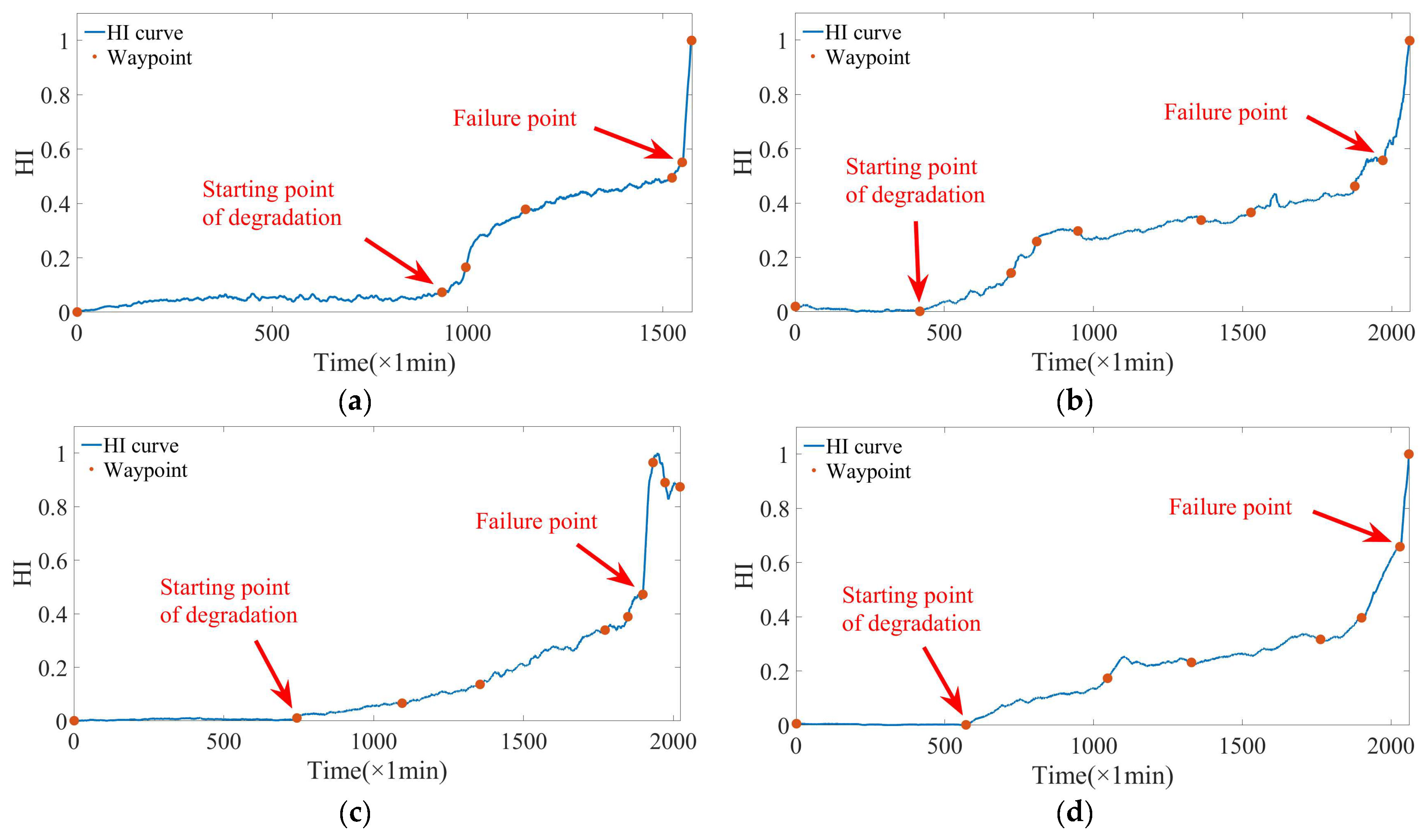
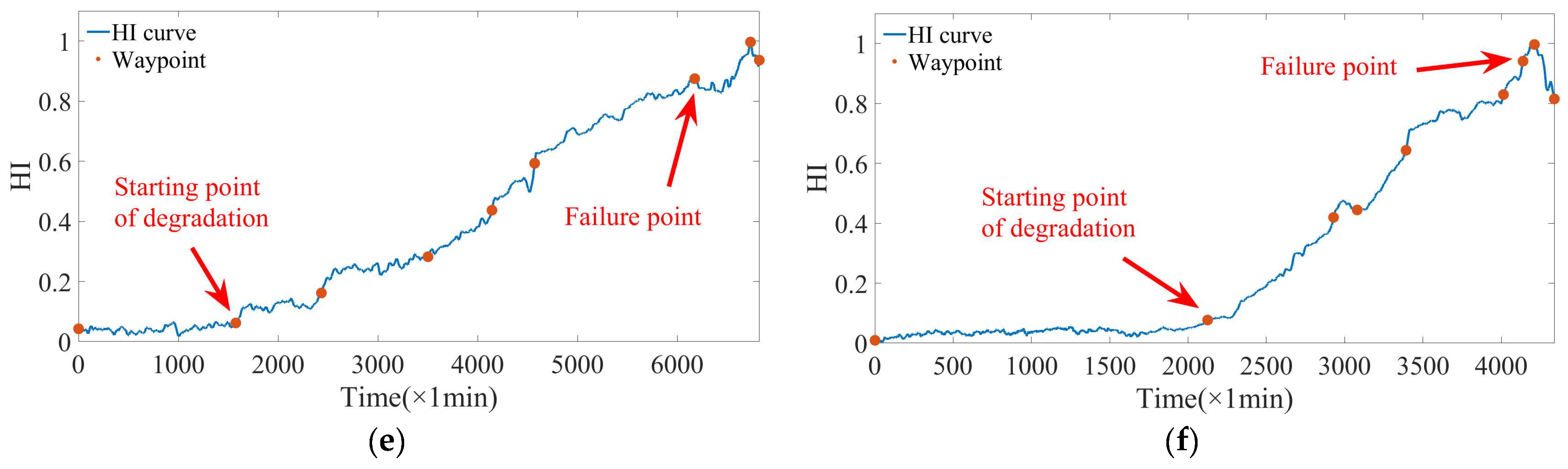
3.2.4. TPD-Based HI Health Status Classification of Rolling Bearings

The health stage of the rolling bearing life cycle contains very little degradation information. At the same time, the health stage and the degradation stage are two distribution trends. It is difficult for the neural network to learn different distributions. The failure stage has lost the meaning of maintenance, so this article only discusses the degradation stage of rolling bearings, that is, the remaining useful life is predicted. An accurate classification of rolling bearing degradation stages can reduce the interference of health status distribution, improve the prediction accuracy of prediction models, prevent misjudgments and waste of computing resources, and play an important role in the subsequent maintenance decisions of rolling bearings. The current commonly used stage division method is the 3σ criterion, and this method is more sensitive to mutation points. When the rolling bearing health status curve has large random fluctuations, using this method is likely to lead to early misjudgment of degradation monitoring points. In this regard, this article introduces a top-down (TPD) timing segmentation method [38]. The flowchart of TPD segmentation is shown in Figure 10. Among these, T is the rolling bearing HI; ς is the algorithm stop threshold Γ = ; and T ˜ is the linear fitting curve of T.

3.3. Simulation Research

In order to verify the effectiveness of this method, a rolling bearing RUL simulation curve was established. The rolling bearing RUL curve can be divided into trend terms and random terms. Combining reference [39] and Figure 11, it can be seen that the degradation process of rolling bearings obeys the inverse Gaussian distribution, so the trend term of the RUL simulation curve of rolling bearings is constructed as x T r e n d = 1 k 1 · exp [ ( ( t k 2 ) / k 3 ) 2 ] . As time goes by, the degradation process of rolling bearings shows more significant nonlinear and random characteristics, which makes the random term of the rolling bearing RUL curve extremely difficult to simulate with conventional functions. In this paper, the random term of the rolling bearing RUL curve is constructed by adding n sine functions and Gaussian white noise. That is, x R a n d = i = 1 n k 4 · sin ( k 5 · t + k 6 ) + η ; the larger n is, xRand is closer to the actual situation. Combined with the actual RUL curve of the rolling bearing, a mathematical model of the rolling bearing RUL simulation curve is constructed, as shown in Equation (20).
t = 1 : 1141 x 1 = 1 1.252 · exp [ ( t 1664 869.5 ) 2 ] x 2 = 0.3315 · sin ( 0.0408 · t 2.667 ) x 3 = 0.3302 · sin ( 0.0409 · t + 0.4522 ) y = x 1 + x 2 + x 3 + η

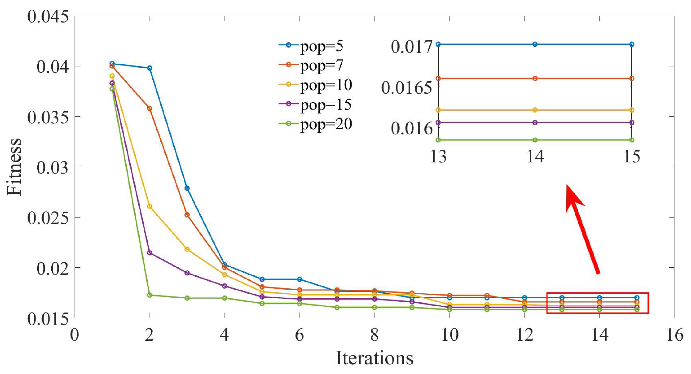
3.3.1. GOA Prediction Model Optimization Parameter Selection

The first 80% of the simulation data are selected as the training set, and the last 20% are the test set. The mean square error between the prediction results and the simulation data is used as the fitness function, the maximum number of iterations is 15, and the number of populations is to be determined. The specific parameter settings for GOA optimization are shown in Table 3, and the fitness curves under different population numbers are shown in Figure 12.
It can be seen from Figure 12 that as the number of populations increases, the corresponding fitness decreases more rapidly in the early iterations and the fitness becomes smaller after the iteration is completed, indicating that increasing the number of GOA populations can increase the optimization effect of the GOA on the TPA-LSTM model parameters. When iterating 12 times, the fitness of all populations has stabilized. Considering that increasing the number of populations will increase the time cost, the number of GOA populations in this article is set to 20.

3.3.2. Simulation Data Prediction Results

In order to verify the prediction effect of each module of the prediction model in this article, the prediction results of the model in this article are compared with the LSTM, GOA-LSTM, and TPA-LSTM models, denoted as M0~M3. Except for the GOA and TPA modules, the structures of each model are consistent. The M1 and M3 model parameters are selected from the initial values in Table 3. In order to describe the prediction effect more intuitively, the root mean square error (RMSE) and the coefficient of determination (R2) are used as evaluation indicators for the prediction results. The calculation method is shown in Equations (21) and (22).
R M S E = 100 · 1 T i = 1 T ( y i y ^ i ) 2
R 2 = 1 i = 1 T ( y i y ^ i ) 2 i = 1 T ( y i y ¯ i ) 2
where T is the size of the data set; yi is the real value; y ^ i is the predicted value; and y ¯ i is the average of the real values. The smaller the RMSE, the higher the prediction accuracy; the smaller the 1 R 2 , the better the fitting effect.
Through calculation, the prediction results of the simulation data training set and test set based on the four prediction models are shown in Table 4, and the prediction curve is shown in Figure 13.
The prediction results of each model in the training set can be seen in Table 4. The RMSE of GOA-LSTM is reduced by 77.57% compared to the traditional LSTM and the RMSE of TPA-LSTM is reduced by 76.76% compared to the traditional LSTM. Compared with the traditional LSTM, the RMSE of this model is reduced by 78.92%, indicating that adding the GOA module or TPA module can improve the prediction accuracy of the model, and this effect can be superimposed. For the prediction results of each model in the test set, the RMSE of GOA-LSTM is reduced by 69.96% compared to the traditional LSTM; the RMSE of TPA-LSTM is reduced by 78.02% compared to the traditional LSTM; the RMSE of the model in this paper is reduced by 87.78% compared to the traditional LSTM, indicating that adding the TPA module can improve the long-term prediction ability of the model, allowing the model to maintain a high accuracy in the later stages of prediction. Combining Table 4 and Figure 13, we can see that traditional LSTM cannot effectively track and predict simulation data starting at 600 min. Compared with the prediction results of its own training set, the R2 of the LSTM test set dropped by 40.51%; the R2 of the GOA-LSTM test set dropped by 2.41%; the R2 of the TPA-LSTM test set dropped by 0.61%; the R2 of the model test set in this article was only a decrease of 0.20%, proving that adding the TPA module can enhance the model’s ability to recognize and remember key time series information and improve the model’s tracking and prediction capabilities.

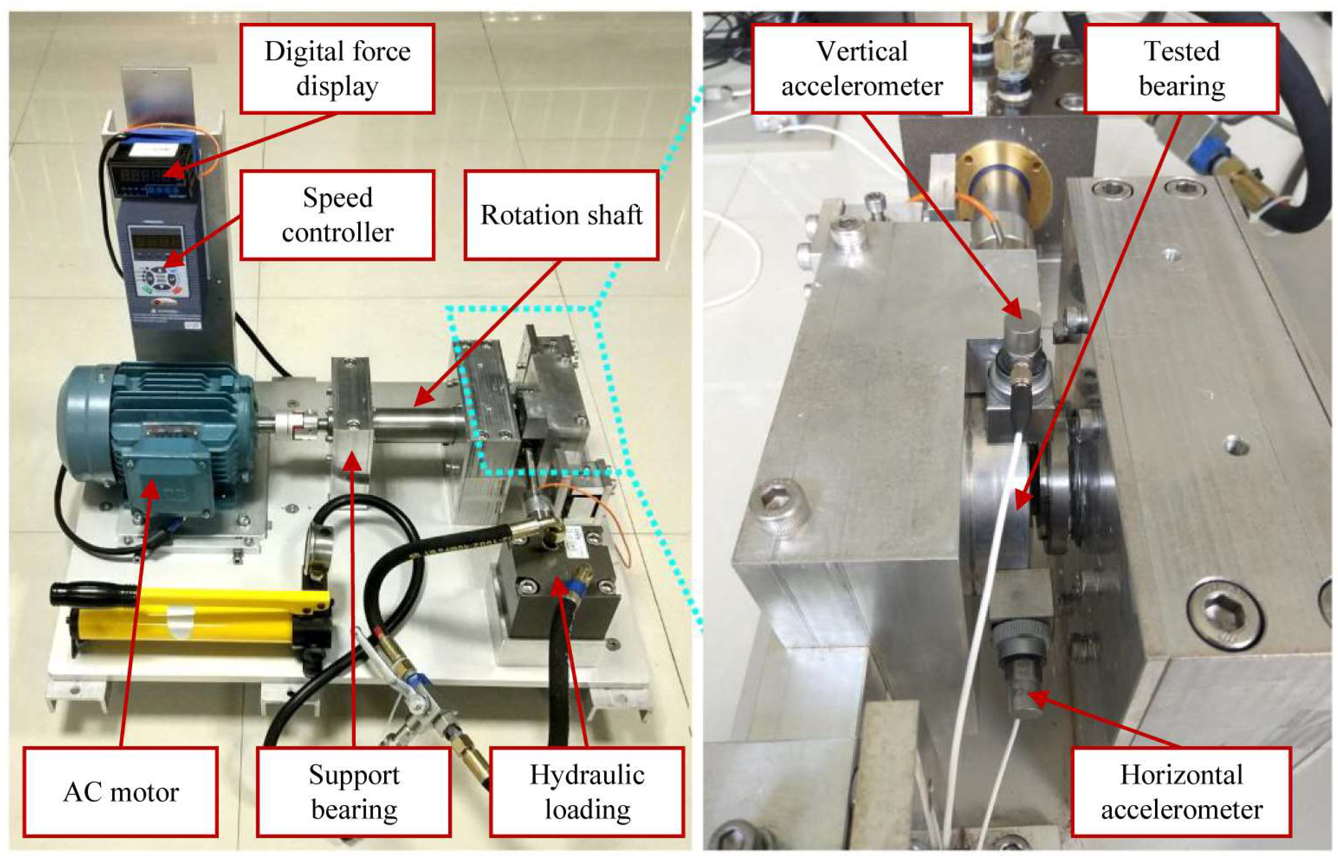
3.4. Experimental Research

In order to verify the actual prediction ability of the rolling bearing RUL of the method in this article, the BiLSTM, CNN-LSTM, and TCN models were used as the control group to form a comparative experiment, denoted as M0~M3. The control group models all used GOA parameters for optimization.
In order to quantify the model prediction uncertainty of the rolling bearing RUL point prediction, quantile regression is integrated with the prediction model. This method retains the nonlinear prediction ability of deep learning while obtaining rolling bearing RUL interval probability prediction. The objective function of the fused prediction model is as follows:
L q ( y i , y i q ) = i = 1 n [ q ( y i q y i ) + ( q 1 ) ( y i q y i ) ]
where yi is the true value; y i q is the predicted value when the quantile is q; and the first term is the objective function when the predicted value is greater than the true value and the second term is the objective function when the predicted value is less than the true value.
In order to obtain the 90% confidence interval of the model prediction, the value of q is [0.1:0.1:0.9] and a total of nine prediction curves form the confidence interval. Use kernel density estimation to obtain the probability density map of the prediction interval and use the predicted values at each quantile as the input value of the kernel density estimation. The probability density function formula is as follows:
f h ( y i ) = 1 n h q = 1 Q K ( y i y i q h )
K ( x ) = 1 2 π exp ( x 2 2 ) h 1.06 · s t d ( y i ) · n 1 5
where n is the total number of samples; Q is the total number of quantiles; K ( · ) is the non-negative kernel function; and h is the sampling bandwidth.
In order to describe the interval prediction effect more intuitively, the prediction interval coverage probability (PICP) and the prediction interval normalized averaged width (PINAW) are used as evaluation indicators for the prediction results. The larger the PICP, the more reliable the model prediction results; the smaller the PINAW, the more reliable the model prediction results and the higher the clarity. The calculation method is shown in Equations (26) and (27).
P I C P = 1 n i = 1 n C i
P I N A W = 1 n y i i = 1 n ( u i l i )
where ui and li are the upper and lower bounds of the prediction interval of the i prediction point, respectively; when the true value y i [ l i , u i ] , Ci = 1, otherwise Ci = 0.
Select the bearings C1 and C2 under the first working condition as the training set and C3 as the test set; select the bearings C4 and C5 under the second working condition as the training set and C6 as the test set. Each type of bearing data is processed through the above Section 3.2 to obtain the degradation stage feature sequence of three fusion features of each type of bearing data, which is projected into the [0, 1] interval as the input of the prediction model, so the input layer dimension of the prediction model is 3, the label expression is as follows:
y i = N i N i [ 1 , N ]
Through calculation, the prediction results of the measured data test set based on the four prediction models are shown in Table 5, the prediction curves are shown in Figure 14 and Figure 15, and the prediction result PDF is shown in Figure 16.
It can be seen from Table 5 that for the prediction results of bearing C3, the RMSE of this method is reduced by 63.26%, 61.24%, and 60.72%, respectively, compared with BiLSTM, CNN-LSTM and TCN; for the prediction results of bearing C6, the RMSE is reduced by 63.26%, 61.24%, and 60.72%, respectively. It shows that the model in this paper can still maintain a high accuracy in prediction on measured data. The TCN model has good prediction results on bearing C6, but the prediction results on bearing C3 are not ideal. However, the prediction results RMSE of this method on bearings under two different working conditions are both lower than four, indicating that the model in this paper has high general accuracy. It is adaptable and can be applied to model prediction under different working conditions.
Combining Table 5 and Figure 14 and Figure 15, it can be seen that for the early and late stages of rolling bearing degradation, the true value is covered by the prediction interval at a higher rate. However, in the middle and late stages of rolling bearing degradation, the prediction interval becomes narrower and the coverage of the true value by the prediction interval becomes lower. This phenomenon is more obvious in bearing C6. In Figure 16b, the model predicts that multiple “peaks” appear in the PDF graph between 1000 and 2000 min, indicating that multiple degradation distributions occur here. This is caused by the fact that different bearings exhibit different states such as gradual or sudden changes from the early stage of degradation to the middle stage of degradation.

4. Conclusions

(1) The LSTM that introduces the TPA and uses GOA parameter optimization strengthens the connection between the hidden layer at different times in the past and the hidden layer at the current time, which is beneficial to improving the long-term series prediction performance of the model. Compared with other networks, the prediction performance of this method is superior and has practical application value.
(2) Using QRLSTM to quantify the uncertainty of RUL prediction results is helpful to quantify decision-making risks when optimizing rolling bearing maintenance decisions. However, through analysis, it is found that the prediction accuracy of this model is affected by the uncertainty of individual bearing differences, and this problem remains to be solved.

Author Contributions

Conceptualization, N.L.; software, Y.T.; validation, Y.T., A.L. and P.J.; formal analysis, Y.T.; investigation, N.L.; writing—original draft preparation, N.L.; writing—review and editing, A.L. and P.J.; supervision, A.L.; project administration, N.L. All authors have read and agreed to the published version of the manuscript.

Funding

This work was supported by the Youth Science Foundation of Northeast Petroleum University (Grant numbers 2018QNL-28).

Data Availability Statement

The datasets used or analyzed during the current study are available from the corresponding author on reasonable request.

Conflicts of Interest

The authors declare that they have no known competing financial interests or personal relationships that could have appeared to influence the work reported in this paper.

References

  1. Rai, A.; Upadhyay, S.H. A review on signal processing techniques utilized in the fault diagnosis of rolling element bearings. Tribol. Int. 2016, 96, 289–306. [Google Scholar] [CrossRef]
  2. Wang, G.; He, Z.; Chen, X.; Lai, Y. Basic research on machinery fault diagnosis—What is the prescription. J. Mech. Eng. China 2013, 49, 63–72. [Google Scholar] [CrossRef]
  3. Peng, C.; Tseng, S. Mis-Specification Analysis of Linear Degradation Models. IEEE Trans. Reliab. 2009, 58, 444–455. [Google Scholar] [CrossRef]
  4. Feng, L.; Wang, H.; Si, X.; Zou, H. A State-Space-Based Prognostic Model for Hidden and Age-Dependent Nonlinear Degradation Process. IEEE Trans. Autom. Sci. Eng. 2013, 10, 1072–1086. [Google Scholar] [CrossRef]
  5. Peng, Y.; Wang, Y.; Zi, Y. Switching State-Space Degradation Model With Recursive Filter/Smoother for Prognostics of Remaining Useful Life. IEEE Trans. Ind. Inform. 2019, 15, 822–832. [Google Scholar] [CrossRef]
  6. Pang, Z.; Si, X.; Hu, C.; Du, D.; Pei, H. A Bayesian Inference for Remaining Useful Life Estimation by Fusing Accelerated Degradation Data and Condition Monitoring Data. Reliab. Eng. Syst. Saf. 2021, 208, 107341. [Google Scholar] [CrossRef]
  7. Lei, Y. Intelligent Fault Diagnosis and Remaining Useful Life Prediction of Rotating Machinery; Butterworth-Heinemann: Amsterdam, The Netherlands, 2016; pp. 12–86. [Google Scholar] [CrossRef]
  8. Tang, Y.; Lin, F.; Zou, L. Research on the fault diagnosis method for reciprocating compressor based on LMD, MSE and LSSVM. Compress. Technol. China 2018, 2018, 1–7. [Google Scholar] [CrossRef]
  9. Wang, R.; Hou, Q.; Shi, R. Residual life prediction method of lithium battery based on variational mode decomposition and integration depth model. Chin. J. Sci. Instrum. 2021, 42, 111–120. [Google Scholar] [CrossRef]
  10. Deutsch, J.; He, D. Using Deep Learning-Based Approach to Predict Remaining Useful Life of Rotating Components. IEEE Trans. Syst. Man Cybern. Syst. 2018, 48, 11–20. [Google Scholar] [CrossRef]
  11. Wang, F.; Liu, X.; Deng, G.; Yu, X.; Li, H.; Han, Q. Remaining Life Prediction Method for Rolling Bearing Based on the Long Short-Term Memory Network. Neural Process. Lett. 2019, 50, 2437–2454. [Google Scholar] [CrossRef]
  12. Zhang, B.; Zhang, L.; Xu, J. Degradation feature selection for remaining useful life prediction of rolling element bearings. Qual. Reliab. Eng. Int. 2016, 32, 547–554. [Google Scholar] [CrossRef]
  13. Tayade, A.; Patil, S.; Phalle, V.; Kazi, F.; Powar, S. Remaining useful life (RUL) prediction of bearing by using regression model and principal component analysis (PCA) technique. Vibroeng. Procedia 2019, 23, 30–36. [Google Scholar] [CrossRef]
  14. Mao, W.; He, J.; Tang, J.; Li, Y. Predicting remaining useful life of rolling bearings based on deep feature representation and long short-term memory neural network. Adv. Mech. Eng. 2018, 10, 1687814018817184. [Google Scholar] [CrossRef]
  15. Li, N.; Lei, Y.; Lin, J.; Ding, S.X. An Improved Exponential Model for Predicting Remaining Useful Life of Rolling Element Bearings. IEEE Trans. Ind. Electron. 2015, 62, 7762–7773. [Google Scholar] [CrossRef]
  16. Jin, X.; Sun, Y.; Que, Z.; Wang, Y.; Chow, T.W. Anomaly Detection and Fault Prognosis for Bearings. IEEE Trans. Instrum. Meas. 2016, 65, 2046–2054. [Google Scholar] [CrossRef]
  17. Wang, L.; Wu, Z.; Fu, Y.; Yang, G. Remaining life predictions of fan based on time series analysis and BP neural networks. In Proceedings of the 2016 IEEE Information Technology, Networking, Electronic and Automation Control Conference, Chongqing, China, 20–22 May 2016; pp. 607–611. [Google Scholar] [CrossRef]
  18. Zhang, Z.; Li, L.; Zhao, W. Tool Life Prediction Model Based on GA-BP Neural Network, Materials Science Forum; Trans Tech Publications Ltd.: Wollerau, Switzerland, 2016; Volume 836–837, pp. 256–262. Available online: https://www.scientific.net/MSF.836-837.256 (accessed on 26 March 2024).
  19. Chen, X.; Xiao, H.; Guo, Y.; Kang, Q. A multivariate grey RBF hybrid model for residual useful life prediction of industrial equipment based on state data. Int. J. Wirel. Mob. Comput. 2016, 10, 90. [Google Scholar] [CrossRef]
  20. Wang, X.; Han, M. Online sequential extreme learning machine with kernels for nonstationary time series prediction. Neurocomputing 2014, 145, 90–97. [Google Scholar] [CrossRef]
  21. Miao, J.; Li, X.; Ye, J. Predicting research of mechanical gyroscope life based on wavelet support vector. In Proceedings of the 2015 First International Conference on Reliability Systems Engineering (ICRSE), Beijing, China, 21–23 October 2015; pp. 1–5. [Google Scholar] [CrossRef]
  22. Babu, G.S.; Zhao, P.; Li, X. Deep Convolutional Neural Network Based Regression Approach for Estimation of Remaining Useful Life, Database Systems for Advanced Applications. In Proceedings of the 21st International Conference, DASFAA 2016, Dallas, TX, USA, 16–19 April 2016; Part 21; Springer International Publishing: Berlin/Heidelberg, Germany, 2016; pp. 214–228. [Google Scholar] [CrossRef]
  23. Zhu, J.; Chen, N.; Peng, W. Estimation of Bearing Remaining Useful Life Based on Multiscale Convolutional Neural Network. IEEE Trans. Ind. Electron. 2019, 66, 3208–3216. [Google Scholar] [CrossRef]
  24. Li, X.; Zhang, W.; Ding, Q. Deep learning-based remaining useful life estimation of bearings using multi-scale feature extraction. Reliab. Eng. Syst. Saf. 2019, 182, 208–218. [Google Scholar] [CrossRef]
  25. Mo, R.; Li, T.; Si, X.; Zhu, X. Remaining useful life prediction for equipment using residual network and convolutional attention mechanism. J. Xi’an Jiaotong Univ. China 2022, 56, 1–9. [Google Scholar] [CrossRef]
  26. Heimes, F.O. Recurrent neural networks for remaining useful life estimation. In Proceedings of the 2008 International Conference on Prognostics and Health Management, Denver, CO, USA, 6–9 October 2008; pp. 1–6. [Google Scholar] [CrossRef]
  27. Guo, L.; Li, N.; Jia, F.; Lei, Y. A recurrent neural network based health indicator for remaining useful life prediction of bearings. Neurocomputing 2017, 240, 98–109. [Google Scholar] [CrossRef]
  28. Wang, B.; Lei, Y.; Yan, T.; Li, N.; Guo, L. Recurrent convolutional neural network: A new framework for remaining useful life prediction of machinery. Neurocomputing 2020, 379, 117–129. [Google Scholar] [CrossRef]
  29. Huang, C.; Huang, H.; Li, Y. A Bidirectional LSTM Prognostics Method Under Multiple Operational Conditions. IEEE Trans. Ind. Electron. 2019, 66, 8792–8802. [Google Scholar] [CrossRef]
  30. Ma, M.; Mao, Z. Deep-Convolution-Based LSTM Network for Remaining Useful Life Prediction. IEEE Trans. Ind. Inform. 2021, 17, 1658–1667. [Google Scholar] [CrossRef]
  31. Bai, S.; Kolter, J.; Koltun, V. An Empirical Evaluation of Generic Convolutional and Recurrent Networks for Sequence Modeling. arXiv 2018, arXiv:1803.01271. [Google Scholar] [CrossRef]
  32. She, D.; Jia, M. A BiGRU method for remaining useful life prediction of machinery. Measurement 2021, 167, 108277. [Google Scholar] [CrossRef]
  33. Jiang, G.; Yang, J.; Cheng, T. Remaining useful life prediction of rolling bearings based on Bayesian neural network and uncertainty quantification. Qual. Reliab. Eng. Int. 2023, 39, 1756–1774. [Google Scholar] [CrossRef]
  34. Shih, S.; Sun, F.; Lee, H. Temporal pattern attention for multivariate time series forecasting. Mach. Learn. 2019, 108, 1421–1441. [Google Scholar] [CrossRef]
  35. Agushaka, J.O.; Ezugwu, A.E.; Abualigah, L. Gazelle optimization algorithm: A novel nature-inspired metaheuristic optimizer. Neural Comput. Appl. 2023, 35, 4099–4131. [Google Scholar] [CrossRef]
  36. Wang, B.; Lei, Y.; Li, N.; Li, N. A Hybrid Prognostics Approach for Estimating Remaining Useful Life of Rolling Element Bearings. IEEE Trans. Reliab. 2020, 69, 401–412. [Google Scholar] [CrossRef]
  37. Wen, J.; Gao, H. A prediction method of bearing residual life based on UPF. J. Vib. Shock. 2018, 37, 208–213. [Google Scholar] [CrossRef]
  38. Eamonn, K.; Selina, C.; David, H.; Michael, P. Segmenting Time Series: A Survey and Novel Approach. In Data Mining in Time Series Databases; World Scientific: Singapore, 2004; pp. 1–21. [Google Scholar] [CrossRef]
  39. Ye, Z.-S.; Chen, N. The inverse gaussian process as a degradation model. Technometrics 2014, 56, 302–311. [Google Scholar] [CrossRef]
Figure 1. LSTM unit structure diagram. Where: f t , i t , o t represent the forget gate, input gate, and output gate of the LSTM unit at time t, respectively.
Machines 12 00224 g001
Figure 2. TPA mechanism structure diagram.
Machines 12 00224 g002
Figure 3. Optimization flow chart of the GOA algorithm.
Machines 12 00224 g003
Figure 4. Overall flow chart of RUL prediction for rolling bearings.
Machines 12 00224 g004
Figure 5. Bearing accelerated life test platform.
Machines 12 00224 g005
Figure 6. Partial feature curves of the bearing C3 feature set.
Machines 12 00224 g006
Figure 7. Indicator stack histogram for each feature of the six bearing data sets: (a) Bearing C1, (b) Bearing C2, (c) Bearing C3, (d) Bearing C4, (e) Bearing C5, (f) Bearing C6.
Machines 12 00224 g007aMachines 12 00224 g007b
Figure 8. Hierarchical clustering dendrogram of six bearing feature sets: (a) Bearing C1, (b) Bearing C2, (c) Bearing C3, (d) Bearing C4, (e) Bearing C5, (f) Bearing C6.
Machines 12 00224 g008
Figure 9. PCA fusion curve of six bearing feature sets: (a) Bearing C1, (b) Bearing C2, (c) Bearing C3, (d) Bearing C4, (e) Bearing C5, (f) Bearing C6.
Machines 12 00224 g009
Figure 10. Flow chart of HI health status division of a rolling bearing based on TPD.
Machines 12 00224 g010
Figure 11. Six types of bearing HIs and stage division results: (a) Bearing C1, (b) Bearing C2, (c) Bearing C3, (d) Bearing C4, (e) Bearing C5, (f) Bearing C6.
Machines 12 00224 g011aMachines 12 00224 g011b
Figure 12. Fitness curves under different population numbers.
Machines 12 00224 g012
Figure 13. Simulation data prediction curves under four prediction models.
Machines 12 00224 g013
Figure 14. RUL prediction curve of bearing C3 under four prediction models: (a) Model M0, (b) Model M1, (c) Model M2, (d) Model M3.
Machines 12 00224 g014
Figure 15. RUL prediction curve of bearing C6 under four prediction models: (a) Model M0, (b) Model M1, (c) Model M2, (d) Model M3.
Machines 12 00224 g015
Figure 16. PDF of test set bearing RUL prediction under this prediction model: (a) Bearing C3, (b) Bearing C6.
Machines 12 00224 g016
Table 1. Test data conditions.
Working ConditionsRotating Speed/r·min−1Radial Force/kN
1210012
2225011
3240010
Table 2. Hierarchical clustering and PCA fusion results of six bearing feature sets.
Bearing LabelsHierarchical Clustering ResultsContribution of Fused Featureavh
ClusterFeature Labels
C1D1F2, F5, F6, F7, F8, F14, F1599.63%0.1280
D2F3, F12, F13, F16, F18, F21, F22, F2395.40%0.2106
D3F10, F17, F1997.26%0.3415
C2D1F2, F5, F6, F7, F8, F14, F1598.54%0.1701
D2F12, F1898.51%0.3551
D3F17, F1999.21%0.2892
C3D1F2, F5, F6, F7, F8, F14, F1599.23%0.1500
D2F4, F1098.38%0.1729
D3F12, F13, F16, F17, F18, F19, F22, F2395.34%0.2642
C4D1F2, F5, F6, F7, F8, F14, F1598.42%0.1793
D2F12, F13, F16, F17, F18, F19, F22, F2395.51%0.2478
D3F20, F2197.77%0.4021
C5D1F2, F5, F6, F7, F8, F14, F1599.61%0.3883
D2F12, F1896.14%0.4845
D3F13, F22, F2395.15%0.3999
C6D1F2, F5, F6, F7, F8, F1599.99%0.2993
D2F14100%0.4214
D3F12100%0.2893
Table 3. GOA parameter settings.
Parameters to be OptimizedInitial ValueOptimization Boundary
LSTM layer units40[20, 200]
Dropout rate0.2[0.1, 0.4]
Training period100[30, 300]
Learning rate0.01[10 × 10−4, 0.1]
Table 4. Simulation data prediction results under four prediction models.
IndexData SetPrediction Model
M0M1M2M3
RMSETraining0.783.700.830.86
Testing0.947.692.311.69
R2Training0.9990.9060.9950.997
Testing0.9970.5390.9710.991
Table 5. Test set bearing RUL prediction results under four models.
BearingIndexPrediction Model
M0M1M2M3
C3RMSE2.3906.5056.1666.084
R20.9930.9500.9550.956
PICP0.7370.4260.4810.467
PINAW0.9651.3180.9260.907
C6RMSE3.94411.1188.0484.509
R20.9810.8610.9230.976
PICP0.4350.1220.1570.524
PINAW0.9430.7370.9060.925
Disclaimer/Publisher’s Note: The statements, opinions and data contained in all publications are solely those of the individual author(s) and contributor(s) and not of MDPI and/or the editor(s). MDPI and/or the editor(s) disclaim responsibility for any injury to people or property resulting from any ideas, methods, instructions or products referred to in the content.

