Nonlinear Passive Observer for Motion Estimation in Multi-Axis Precision Motion Control

Abstract

A nonlinear passive observer (NPO) for estimating the time-varying velocity vector of a multi-axis high-precision motion control stage is presented. The proposed nonlinear estimation strategy is developed based on a Lyapunov stability analysis, which proves that the NPO is stable. Three test cases are used to investigate the performance of the proposed observer. Experimental results are given to demonstrate the performance of the proposed NPO in accurately estimating time-varying velocity during alignment, reciprocating motion, and multi-axis motion in high-precision motion control applications.

1. Introduction

Several control designs have been proposed in the last few years to meet increasing demands on high-precision motion control, in particular 6-DOF stages for ultrahigh-precision-positioning applications such as photolithography and semiconductor fabrication. In 6-DOF stages based on magnetic suspension devices with a small range of motion, the dynamics are often assumed to be decoupled: independent SISO models are assumed to describe each axis of motion, and lead–lag compensators are used to control each SISO model [1,2]. However, coupling between axes becomes significant as the range increases: 6-DOF free-body dynamics of a moving mass are inherently highly nonlinear and coupled. On the other hand, often in high-precision positioning applications only position and not direct velocity measurements are available. To reduce dynamic coupling, a multivariable LQ controller that uses three velocity feedback signals was used by Shakir et al. [3]. For long-range trajectory tracking, advanced controls have been proposed. For instance, in applications that involve continuous directional changes in the planned trajectory such as direct-write nanopatterning, it is crucial to have velocity control in addition to position control [2,3]. Time-optimal control or bang–bang control is often desirable if fast motion and high throughput are required.

Advanced control schemes such as feedback linearization and sliding mode control require full state feedback, which can be impractical or unfeasible [4,5,6,7]. When a direct position is measured (e.g., by a laser interferometer or linear glass scales), the linear and rotary velocities can be measured at the same time by the corresponding interface board [2]. When indirect position feedback is used, state observers can be used to estimate velocity as needed by the feedback law.

Model-based motion estimation has been used in many areas, such as mobile robotics, visual servo control, and servo navigation. Sometimes, even if velocity information can be measured directly, it may not be the preferred option because of measurement noise and/or a low data-update rate. A state estimator could be used instead to distinguish between true motion and measurement noise [8]. In linear systems, state estimation based on noisy measurements is possible using a Kalman filter [9,10]. In nonlinear systems, an extended Kalman filter in the form of high-order nonlinear differential equations can be used but with only local stability guaranteed [11]. Dini and Saponara [12,13] showed that the extended Kalman filter (EKF) may work very well in nonlinear systems that are affine in the input linearized by feedback linearization, such as cogging torque models.

1.1. Review of Nonlinear Observers

A sliding observer, robust to uncertainties and disturbances, has been presented in [14,15,16,17]. However, oscillatory estimation due to high-frequency switching can be an issue with this kind of observer. A 3-DOF nonlinear observer based on a passivity theorem that can produce globally exponentially stable estimates of position and velocity was reported in [18]. In [19,20,21,22,23], high-gain observers that work for a special class of nonlinear systems are discussed. A constant state coefficient matrix in a dynamic system facilitates stability analysis using a classical design approach. This method cannot be used if the state coefficient matrix is time-varying or depends on the system state itself: in that case, a Lyapunov-based method can be used, as proposed in this paper.

Passivity is an energy-related concept that has been of great interest in the analysis of nonlinear systems: by introducing the notions of storage function and supply rate [24,25], less conservativeness in the demonstration of robust stability is needed. On the other hand, observer design based on passivity has rarely been discussed [26]. Passivity can guarantee the existence of a high-gain robust observer in a class of nonlinear uncertain systems [26].

Several recent efforts have used passivity to demonstrate robustness and the global exponential stability of nonlinear observers. Yang et al. [27] presented a robust nonlinear observer for a ship positioning system based on a sliding mode that estimates the low-frequency position and velocity of a vessel from noisy position measurements. Xie et al. [28] introduced a nonlinear passive observer to filter high-frequency disturbances on a measured position and heading of a ship, as well as to estimate the vessel’s velocity. The global exponential stability of the proposed observer was demonstrated based on the satisfaction of a Lyapunov condition [20].

Several works have relied on passivity to guarantee the stability of a nonlinear observer. Alvarez-Salas et al. [29] describe a passive speed observer for the sensorless control of induction motors, and show that its performance is better than an observer based on a model reference adaptive system technique. Almeida et al. [30] uses two observers designed using a generalized high-order sliding mode algorithm to estimate both the unmeasurable states and the operation point of a synchronous generator connected to an infinite bus.

Early observer design for dynamic positioning focused on linear optimal observer design from linearized equations of motion. Due to the lack of global stability, the research shifted to nonlinear observer design, with the disadvantage that optimality is not guaranteed. Snijders et al. [31] presented an optimal nonlinear observer based on contraction theory that achieves optimality at the expense of losing global asymptotic stability. A suboptimal observer using a state-dependent Riccati equation approach was also presented, and both optimal and sub-optimal observers were compared to an existing nonlinear observer.

Nonlinear observers have been extensively studied in the field of dynamic ship positioning. Liu et al. [32] presented a nonlinear observer design that solves the problem caused by a traditional Kalman filter, which needs to linearize kinematic equations, and provides global stability as proven by Lyapunov stability theory; all estimates of ship motion states converge exponentially to the actual values. Lin et al. [33] proposed a nonlinear passive robust observer for a ship dynamic positioning system based on augmenting a new state and utilizing acceleration feedback. The observer improves disturbance attenuation performance, and both global stability and passivity of the observer are demonstrated, as well as performance in numerical simulations. Xia and Shao [34] use a passive nonlinear observer as proposed by Fossen [35] to eliminate high-frequency contents in a ship’s position and heading; the observer can also estimate the low-frequency motions of the ship.

Xie et al. [36] used a nonlinear passive observer and a PD controller to improve the performance of a ship’s dynamic positioning system under extreme environmental conditions. The environmental force, estimated by the proposed observer, acts on bias compensation control, improving the dynamic response of the closed-loop system by attenuating the negative effects from thruster action, which is a high-frequency disturbance. Lyapunov stability theory and a global stability method of nonlinear cascade systems are used to prove the stability of the closed-loop system.

Tong et al. [37] presented two nonlinear observers for estimating attitude and gyro bias using gyro and inertial vector measurements. One is a passive observer, which decouples the gyro measurements from the reconstructed attitude, and the other is the explicit observer evolving on SO(3), which uses body-frame measurements of known inertial vectors. The proposed observers achieve faster convergence for large attitude estimation errors than similar observers in the literature, guarantee asymptotical stability for almost arbitrary initial conditions, and achieve similar steady-state performance with a lower computational cost than an extended Kalman filter.

In this paper, we extend the work from [18] and propose a modified nonlinear passive observer that can provide six-axis motion estimation for high-precision motion control based on a Lyapunov method. Compared to a conventional Kalman filter, a smaller number of tuning parameters is needed since no linearization of the kinematic equations is necessary, and global stability is achieved.

1.2. Multi-Axis High-Precision Motion Control System

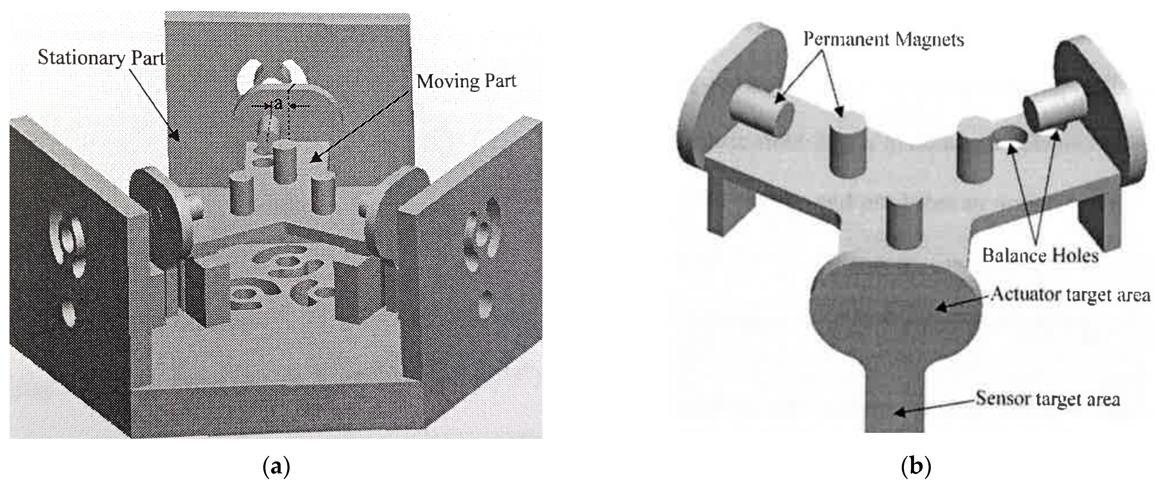
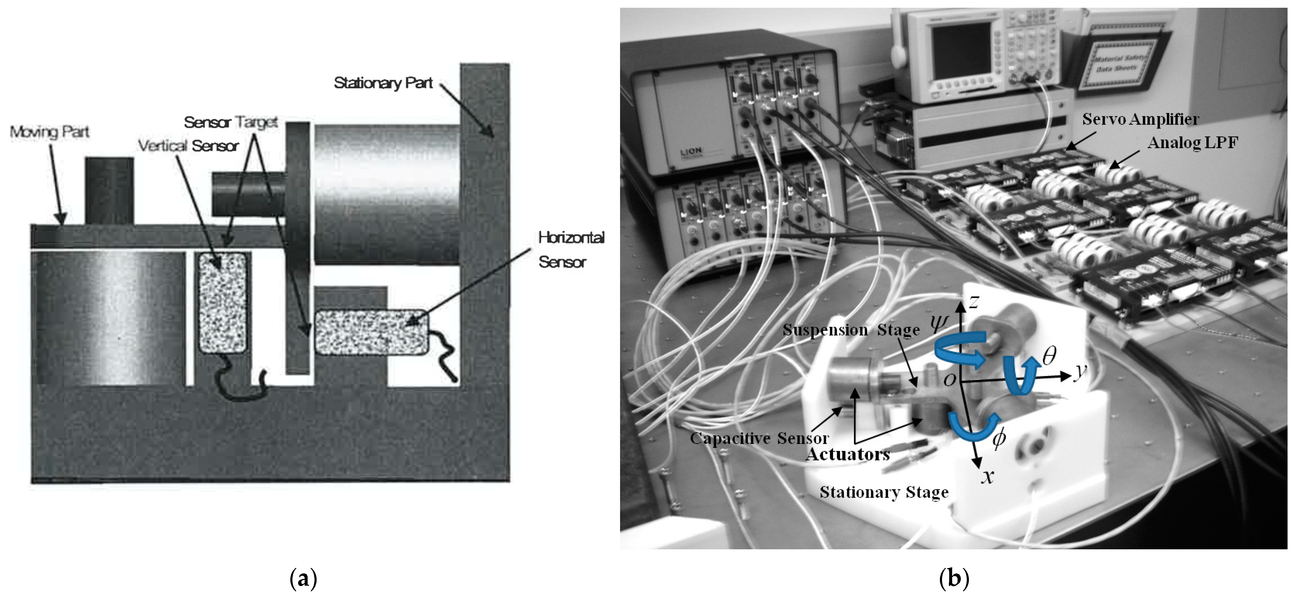
1.2.1. Electromagnetic Long-Range 6-DOF Motion Stage

The proposed technique is demonstrated on a high-precision motion control stage driven by six long-range (up to 1000 μm travel) hybrid magnetic suspension actuators (HMSA) [38,39]. The electromagnetic suspension stage consists of a moving part and a stationary part, as shown in Figure 1; the moving part levitates relative to the stationary part with the 6-DOF position and orientation controlled by six electromagnets, three located on the sides of the stator, and three located at the base, as shown in Figure 2.

HSMA use a combination of passive and active electromagnetic forces to provide long-range actuation. The position and orientation of the motion stage are controlled in a fashion similar to a Stewart platform, with six independent force actuators and six corresponding air gaps measured by capacitive sensors, as shown in Figure 2a. The 6-DOF position and orientation of the motion stage can be estimated based on the six air gap readings where the nominal range for each gap is from 500 to 1500 μm. To avoid the singularity inherent in symmetrical Stewart platforms, one of the permanent magnets in the motion stage is placed with an “a” offset, as shown in Figure 1a. This offset affects the mass distribution relative to the body frame of the motion stage, introducing non-zero product-of-inertia terms in the inertia tensor. To compensate for the unbalanced mass distribution, two balance holes are introduced (Figure 1b) by changing their dimensions and location until the product-of-inertia terms are negligible compared to the principal moments of inertia, such that the inertia matrix is as close as possible to diagonal.

The moving part (Figure 1b) consists of ferromagnetic pole pieces that interact with the electromagnets, and supports permanent magnet stacks and sensor target areas for the capacitance probes. The sensor target areas are flat and at least 30% larger than the sensor’s sensing surface to achieve the highest accuracy.

The motion stage uses six capacitive sensors to estimate the 6-DOF motion of the moving part. Three horizontal and three vertical hybrid electromagnetic actuators are used to drive the levitated platform. HMSA are coaxial actuators that combine permanent magnets and coil drivers to provide precision positioning by controlling coil currents. Several strategies including MIMO PD tracking control and sliding mode control have been proposed to control this type of motion stage [39]. By using position feedback from six capacitive sensors and adjusting the current passing through each actuator, control of the 6-DOF motion of the suspension stage can be achieved. The mass properties of the suspension stage are shown in

Table 1. Physical specifications of the suspension stage, Figure 1b.

Range of motion <X,Y,Z>	+/−0.001	m
Mass	$m=0.931$	kg
Inertia	$I_x=1.799\times {10}^{-3}$ $I_y=1.834\times {10}^{-3}$ $I_z=3.336\times {10}^{-3}$ $I_{xy}\approx 0$, $I_{yz}\approx 0$, $I_{xz}\approx 0$	$\mathrm{K}\mathrm{g}·{\mathrm{m}}^2$

.

1.2.2. Rigid Body Dynamics of the 6-DOF Motion Stage

Consider the body frame {B} attached to the center of gravity of the moving part, and the fixed frame {F} attached to the stationary part (xyz axes in Figure 2b). In the initial configuration (all six air gaps equal to 1 mm, with all rotation angles equal to zero), {B} and {F} coincide. Denote the force vector expressed in the body frame as ${}^{B}F$, and the velocity vector of the center of gravity of the moving part with respect to the fixed frame, expressed in body coordinates, as ${}^{B}V$. The translational dynamics of the moving stage are given as:

$${}^{B}F={}^F\left(\frac{d}{dt}(m{}^{B}V)\right)=m{}^F\left(\frac{d}{dt}{}^{B}V\right)$$

(1)

where ${}^F\left(.\right)$ denotes the derivative of a vector with respect to the fixed frame. Consider now $\Omega$, the angular velocity of the moving stage with respect to the fixed frame. Applying the Coriolis theorem to the translational dynamics shown above, and considering the total force acting on the moving part as the summation of actuator forces F_i plus gravity ${}^{B}G$, the following equation is yielded:

$${}^{B}F=m\left(\frac{d}{dt}{}^{B}V+{}^B\Omega \times {}^{B}V\right)={}^{B}G+\sum {}^{B}F_i$$

(2)

With this, the translational dynamics of the moving part are:

$$\frac{d}{dt}{}^{B}V=\frac{1}{m}\left({}^{B}G+\sum {}^{B}F_i\right)-{}^B\Omega \times {}^{B}V$$

(3)

The rotational dynamics of the moving part are described by Euler’s equation [39]:

$${}^{B}T=I\frac{d}{dt}{}^B\Omega +{}^B\Omega \times I{}^B\Omega$$

(4)

The total torque acting on the moving part is the sum of torques produced by the six hybrid magnetic actuators. With this, the rotational dynamics of the moving part becomes:

$$\frac{d}{dt}{}^B\Omega =I^{-1}\sum {}^{B}T_i-{}^B\Omega \times I{}^B\Omega$$

(5)

The translational and rotational dynamics shown above, subject to the initial conditions $\left({}^{B}V\left(t_o\right), {}^B\mathsf{\Omega }\left(t_o\right) \right)\in \mathbb{R}\times \mathbb{R}$, is an autonomous initial value problem (IVP) that describes the evolution of the moving part of the motion stage. Since this IV is nonlinear and not separable, an analytical solution is not available.

1.2.3. Sliding Mode Controller Design of the 6-DOF Motion of the Moving Part

Sliding mode control is widely used in applications where system parameters and unmodelled dynamics have bounded uncertainties [20,38,39]. To account for modeling and parametric uncertainty, the control law is defined as discontinuous across the sliding surface. This tends to induce chatter or even unmodelled high-frequency dynamics; in practice, a boundary layer of arbitrarily small thickness is defined in the proximity of the sliding surface to smooth out discontinuity of the control action. Outside the boundary layer, the control input u is selected so that the boundary layer is attractive, while inside the boundary layer, u is interpolated as a smooth function. Bounds on the sliding surface can be directly translated into bounds on the tracking error [20]; a trade-off must be made between tracking precision and robustness and unmodelled dynamics and parametric uncertainty.

The use of observers in high-precision positioning systems such as those used in semiconductor manufacturing has been discussed in the literature. Wang et al. [40] presented an extended state observer used on a run-to-run (RtR) controller to suppress stochastic disturbances emerging in semiconductor manufacturing processes. The observer is used to estimate process disturbances, rather than kinematic states of the motion stage. Similarly, Lee et al. [41] present an output disturbance observer that reduces sensitivity to modeling errors and enhances disturbance rejection of the overall motion controller. Tsai and Peng [42] developed a sliding mode observer for the estimation of core temperature in multi-layer plates in semiconductor manufacturing. In [43], a model of the hybrid magnetic actuator’s axial force as a function of an air gap and coil current is presented, together with a high-gain state observer used to estimate velocity from position measurements. Observer-based sliding mode control (quasi-sliding control with reaching law) was introduced in [44] for a 6-DOF positioning system based on the hybrid magnetic actuator used in this study; observer design focuses on the kinematics and excludes the actuator model.

To define the sliding mode control of the positioning stage, define first the total velocity vector ${}^B\mathbb{V}$ expressed in the body frame as follows:

$$\left[\begin{array}{c}{}^B\mathbf{V}\\ {}^B\mathsf{\Omega }\end{array}\right]={}^B\mathbb{V}={\left[\begin{array}{ccc}u& v& w\end{array} \begin{array}{ccc}p& q& r\end{array}\right]}^T$$

(6)

Replacing this expression in the translational dynamics of the moving part defined above yields the following:

$$\left[\begin{array}{c}\dot{u}\\ \dot{v}\\ \dot{w}\end{array}\right]=\frac{1}{m}\left[\begin{array}{c}{{}^{B}F}_x\\ {{}^{B}F}_y\\ {{}^{B}F}_z\end{array}\right]+\frac{1}{m}{}_F{}^B\mathit{R}\left[\begin{array}{c}0\\ 0\\ -mg\end{array}\right]-\left[\begin{array}{c}p\\ q\\ r\end{array}\right]\times \left[\begin{array}{c}u\\ v\\ w\end{array}\right]$$

(7)

where ${}_F{}^B\mathit{R}$ is the 3 × 3 rotation matrix that provides the transformation from fixed coordinates to body coordinates following the z-y-x Euler angle convention (rotation about z by yaw, followed by rotation about y by pitch, followed by rotation about x by roll).

Define the position error in the fixed frame as $\mathit{e}={\mathit{P}}_r-\widehat{\mathit{P}}$, and the velocity error in the fixed frame as $\mathit{c}={\mathbb{V}}_r-\widehat{\mathbb{V}}$, where ${\mathit{P}}_r$ and ${\mathbb{V}}_r$ are the reference position and reference velocity in the fixed frame, and $\widehat{\mathit{P}}$ and $\widehat{\mathbb{V}}$ are the corresponding estimated position and velocity. The sliding surface is defined as $\mathbb{S}=\dot{\mathit{e}}+{\mathsf{\Lambda }}_{6\times 1}\mathit{e}$, and its time derivative is as follows:

$$\dot{\mathbb{S}}=\dot{{\mathbb{V}}_r}-\left[\begin{array}{cc}{}_R{}^F\mathit{R}& 0\\ 0& \mathbf{E}\end{array}\right]\dot{{}^B\mathbb{V}+}{\mathsf{\Lambda }}_{6\times 1}\dot{\mathit{e}}$$

(8)

where ${}_R{}^F\mathit{R}$ is used to transform the translation velocity vector from the body frame to the fixed frame, and E is used to transform the rotational velocity vector expressed in the body frame to the corresponding Euler rates, as defined in Appendix A. A detailed development of the sliding controller for the 6-DOF motion stage has been presented in Refs. [38,39]; in this paper, the focus is the development of a nonlinear passive observer as needed to implement the full-state sliding controller.

1.2.4. Nonlinear Observer Equations

Highly coupled 6-DOF multi-axis motion has often been assumed to be six independent decoupled motions [1,2,45,46,47,48]. Since this is a significant factor that contributes to modeling error, the Newton–Euler Equation (9) (which introduces coupling between axes) is proposed. In Figure 1a, the body frame attached to the levitated stage coincides initially with the inertial frame. The kinematics Equation (10) can be used to relate the position vector P to the velocity vector expressed in the body frame,${}^{B}V$. $M$, $C$, ${}_B{}^F\mathit{R}$, $\mathit{E}$ are the mass matrix, Coriolis matrix (and centrifugal terms), position transformation matrix, and velocity transformation matrix, respectively, as listed in Appendix A. F is the total actuator force expressed in the body frame:

$$M{}^B\dot{V}+C\left({}^{B}V\right){}^{B}V=F$$

(9)

$$\dot{\mathit{P}}=\left[\begin{array}{cc}{}_B{}^F\mathit{R}& \mathit{O}\\ \mathit{O}& \mathit{E}\end{array}\right]{}^B\mathit{V}$$

(10)

The velocity estimates, expressed in the body frame, and position estimates, expressed in the inertial frame, are as follows:

$${}^B\widehat{\mathit{V}}={\left[\begin{array}{cccccc}\widehat{u}& \widehat{v}& \widehat{w}& \widehat{p}& \widehat{q}& \widehat{r}\end{array}\right]}^T$$

$$\widehat{\mathit{P}}={\left[\begin{array}{cccccc}\widehat{x}& \widehat{y}& \widehat{z}& \widehat{\varphi }& \widehat{\theta }& \widehat{\psi }\end{array}\right]}^T$$

Then, a nonlinear velocity observer can be written as follows:

$$\mathit{M}{}^B\dot{\widehat{\mathit{V}}}=\mathit{F}-\mathit{C}\left({}^B\mathit{V}\right){}^B\widehat{\mathit{V}}+{\mathit{D}}_0\left(\mathit{Z}-\widehat{\mathit{P}}\right)$$

(11)

$${\widehat{\mathit{Y}}}_1={}^B\widehat{\mathit{V}}$$

(12)

$$\dot{\widehat{\mathit{P}}}=\left[\begin{array}{cc}{}_B{}^F\mathit{R}& \mathit{O}\\ \mathit{O}& \mathit{E}\end{array}\right]{}^B\mathit{V}+{\mathit{A}}_0\left(\mathit{Z}-\widehat{\mathit{P}}\right)$$

(13)

$${\widehat{\mathit{Y}}}_2=\widehat{\mathit{P}}$$

(14)

where Z is the measured position vector, and ${\mathit{D}}_0 \mathrm{a}\mathrm{n}\mathrm{d} {\mathit{A}}_0$ are tunable gain matrices described in Appendix A.

1.2.5. Stability and Passivity of the Observer

Subtracting Equations (11) and (13) from (9) and (10) gives the error dynamics of the 6-DOF motion estimation:

$$\mathit{M}{}^B\dot{\tilde{\mathit{V}}}=-\mathit{C}\left({}^B\mathit{V}\right){}^B\tilde{\mathit{V}}-{\mathit{D}}_0\tilde{\mathit{P}}$$

(15)

$${\tilde{\mathit{Y}}}_1={}^B\tilde{\mathit{V}}$$

(16)

$$\dot{\tilde{\mathit{P}}}={\mathit{A}}_0\tilde{\mathit{P}}+\left[\begin{array}{cc}{}_B{}^F\mathit{R}& \mathit{O}\\ \mathit{O}& \mathit{E}\end{array}\right]{}^B\tilde{\mathit{V}}$$

(17)

$${\tilde{\mathit{Y}}}_2=\tilde{\mathit{P}}$$

(18)

where $\tilde{\mathbf{P}}$ is the estimation error in the position vector and ${}^B\tilde{\mathbf{V}}$ is the estimation error in the velocity vector, expressed in the body frame.

Proposition 1. 

${\left({\mathit{D}}_0\tilde{\mathit{P}}\right)}^T{}^B\tilde{\mathit{V}}={}^B{\tilde{\mathit{V}}}^T{\mathit{D}}_0\tilde{\mathit{P}}$

Proof. 

Let

$${}^B\tilde{\mathit{V}}={\left[\begin{array}{cccccc}\mathsf{\Delta }{v}_1& \mathsf{\Delta }{v}_2& \mathsf{\Delta }{v}_3& \mathsf{\Delta }{v}_4& \mathsf{\Delta }{v}_5& \mathsf{\Delta }{v}_6\end{array}\right]}^T$$

$$\tilde{\mathit{P}}={\left[\begin{array}{cccccc}\mathsf{\Delta }{p}_1& \mathsf{\Delta }{p}_2& \mathsf{\Delta }{p}_3& \mathsf{\Delta }{p}_4& \mathsf{\Delta }{p}_5& \mathsf{\Delta }{p}_6\end{array}\right]}^T$$

$$\begin{gathered} {\left({\mathit{D}}_0\tilde{\mathit{P}}\right)}^T{}^B\tilde{\mathit{V}}=\sum _{i=1}^6\mathsf{\Delta }{v}_i{d}_i\mathsf{\Delta }{p}_i \\ ={}^B{\tilde{\mathit{V}}}^T{\mathit{D}}_0\tilde{\mathit{P}} \end{gathered}$$

□

Proposition 2. 

${}^B{\tilde{\mathit{V}}}^T\left(\mathit{C}+{\mathit{C}}^T\right){}^B\tilde{\mathit{V}}=0$

Proof. 

$$\begin{gathered} {}^B{\tilde{\mathbf{V}}}^T\left(\mathbf{C}+{\mathbf{C}}^T\right){}^B\tilde{\mathbf{V}} \\ ={}^B{\tilde{\mathbf{V}}}^T\mathbf{O}{}^B\tilde{\mathbf{V}}=0 \end{gathered}$$

□

Proposition 3. 

The velocity observer (3) is passive.

Proof. 

Let $\mathit{u}=-{\mathit{D}}_0\tilde{\mathit{P}}\hspace{1em}\mathit{y}={}^B\tilde{\mathit{V}}$

Consider the Lyapunov candidate:

$$S=\frac{1}{2}{}^B{\tilde{\mathit{V}}}^T\mathit{M}{}^B\tilde{\mathit{V}}$$

□

Differentiating S with respect to time along the trajectory of ${}^B\tilde{V}$ yields the following:

$$\begin{array}{cc}\hfill \dot{S}& =\frac{1}{2}{\left(\mathit{M}{}^B\dot{\tilde{\mathit{V}}}\right)}^T{}^B\tilde{\mathit{V}}+\frac{1}{2}{}^B{\tilde{\mathit{V}}}^T\mathit{M}{}^B\dot{\tilde{\mathit{V}}}\hfill \\ & =\frac{1}{2}{\left(-\mathit{C}{}^B\tilde{\mathit{V}}-{\mathit{D}}_0\tilde{\mathit{P}}\right)}^T{}^B\tilde{\mathit{V}}+\frac{1}{2}{}^B{\tilde{\mathit{V}}}^T\left(-\mathit{C}{}^B\tilde{\mathit{V}}-{\mathit{D}}_0\tilde{\mathit{P}}\right)\hfill \\ & =-\frac{1}{2}{}^B{\tilde{\mathit{V}}}^T{\mathit{C}}^T{}^B\tilde{\mathit{V}}-\frac{1}{2}{\left({\mathit{D}}_0\tilde{\mathit{P}}\right)}^T{}^B\tilde{\mathit{V}}-\frac{1}{2}{}^B{\tilde{\mathit{V}}}^T\mathit{C}{}^B\tilde{\mathit{V}}-\frac{1}{2}{}^B{\tilde{\mathit{V}}}^T{\mathit{D}}_0\tilde{\mathit{P}}\hfill \\ & =-\frac{1}{2}{}^B{\tilde{\mathit{V}}}^T\left({\mathit{C}}^T+\mathit{C}\right){}^B\tilde{\mathit{V}}-\frac{1}{2}\left({\left({\mathit{D}}_0\tilde{\mathit{P}}\right)}^T{}^B\tilde{\mathit{V}}+{}^B{\tilde{\mathit{V}}}^T{\mathit{D}}_0\tilde{\mathit{P}}\right)\hfill \end{array}$$

Applying Propositions 1 and 2 yields:

$$\dot{S}=-{\left({\mathit{D}}_0\tilde{\mathit{P}}\right)}^T{}^B\tilde{\mathit{V}}={\mathit{u}}^T\mathit{y}$$

$${\int }_{t_0}^t{\mathit{u}}^T\left(\tau \right)\mathit{y}\left(\tau \right)d\tau =\frac{1}{2}{}^B{\tilde{\mathit{V}}}^T\mathit{M}{}^B\tilde{\mathit{V}}\ge \delta {}^B{\tilde{\mathit{V}}}^T{}^B\tilde{\mathit{V}}$$

(19)

where δ is a positive constant dependent on the mass matrix. Equation (19) shows that the proposed velocity observer is passive and hence stable.

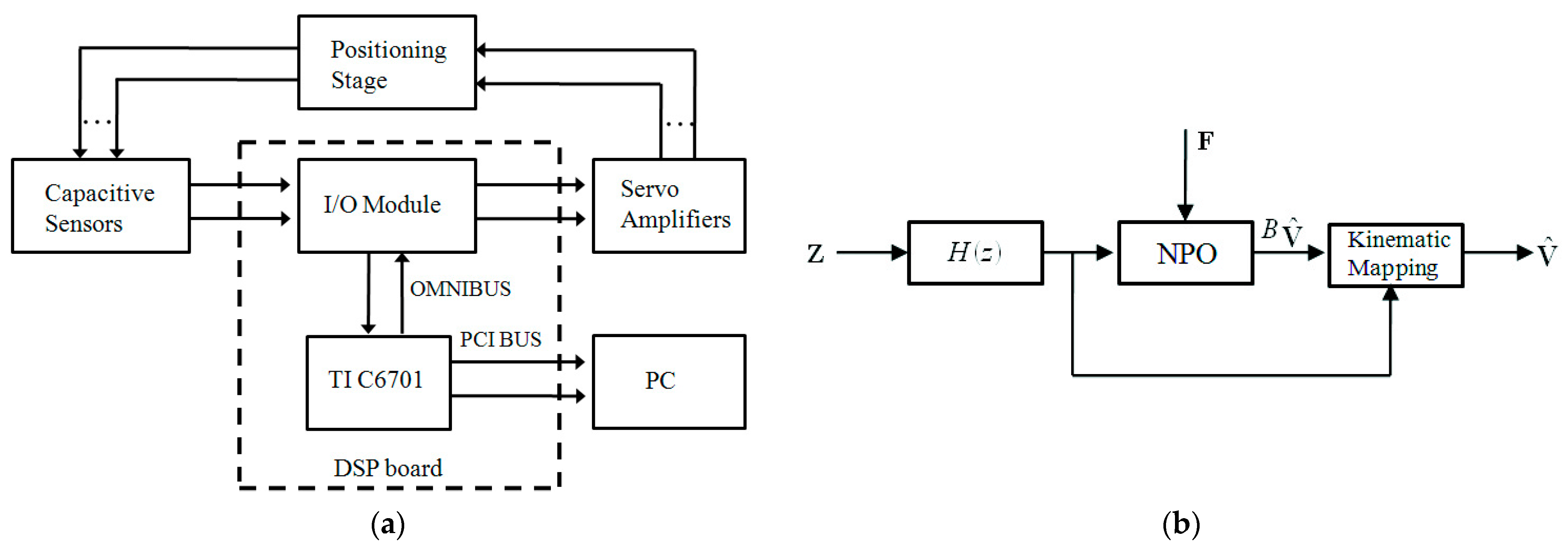
2. Materials and Methods

To assess the multi-axis estimation performance of the proposed observer, several experiments were completed where estimated velocities were compared to velocity estimates calculated by finite differences using filtered position measurements. The observer was implemented on a TI TMS320C67 DSP board (Figure 3a) at a sampling rate of 2.5 kHz. A second-order digital low-pass filter with a linear phase design was used per axis (Figure 3b).

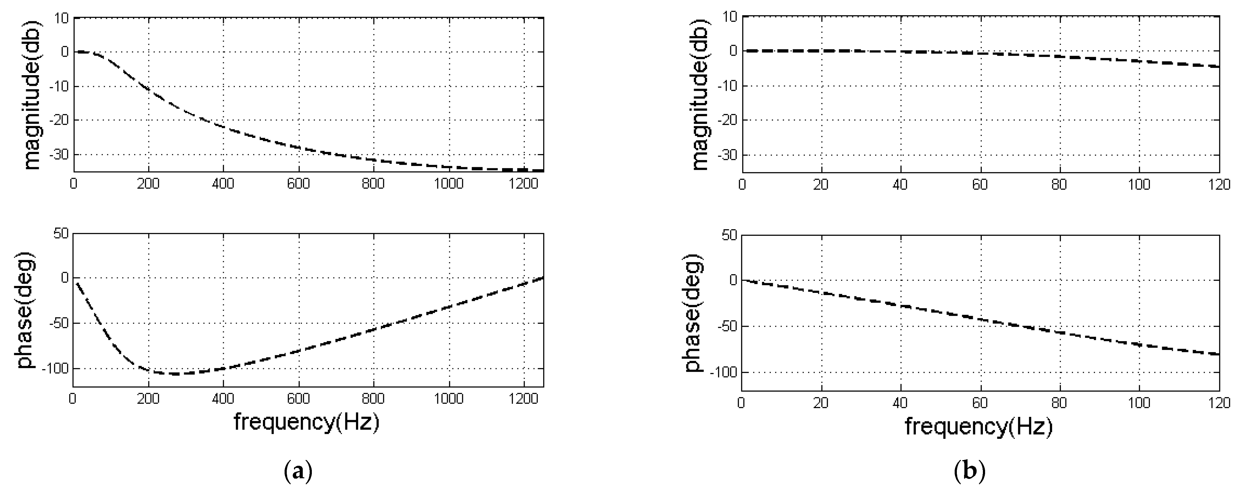
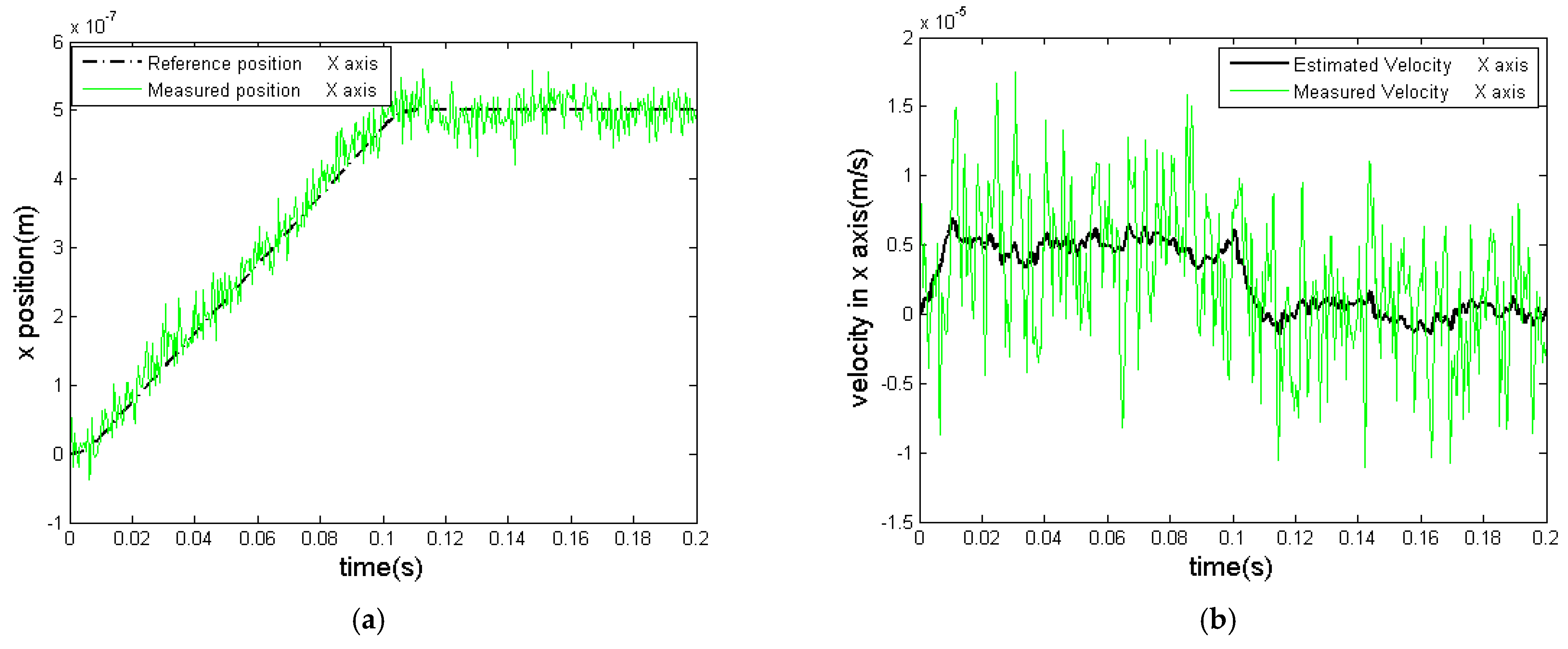
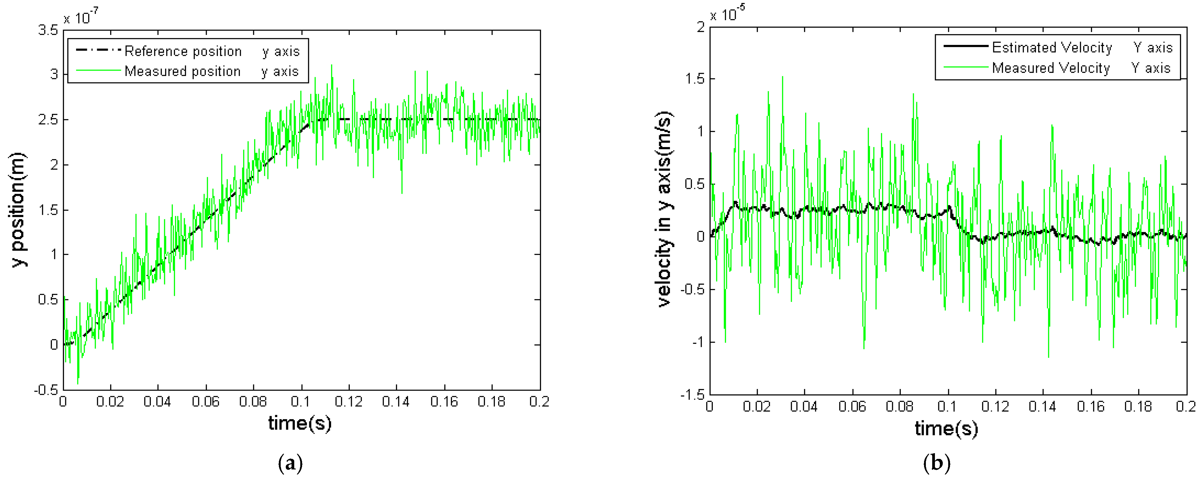
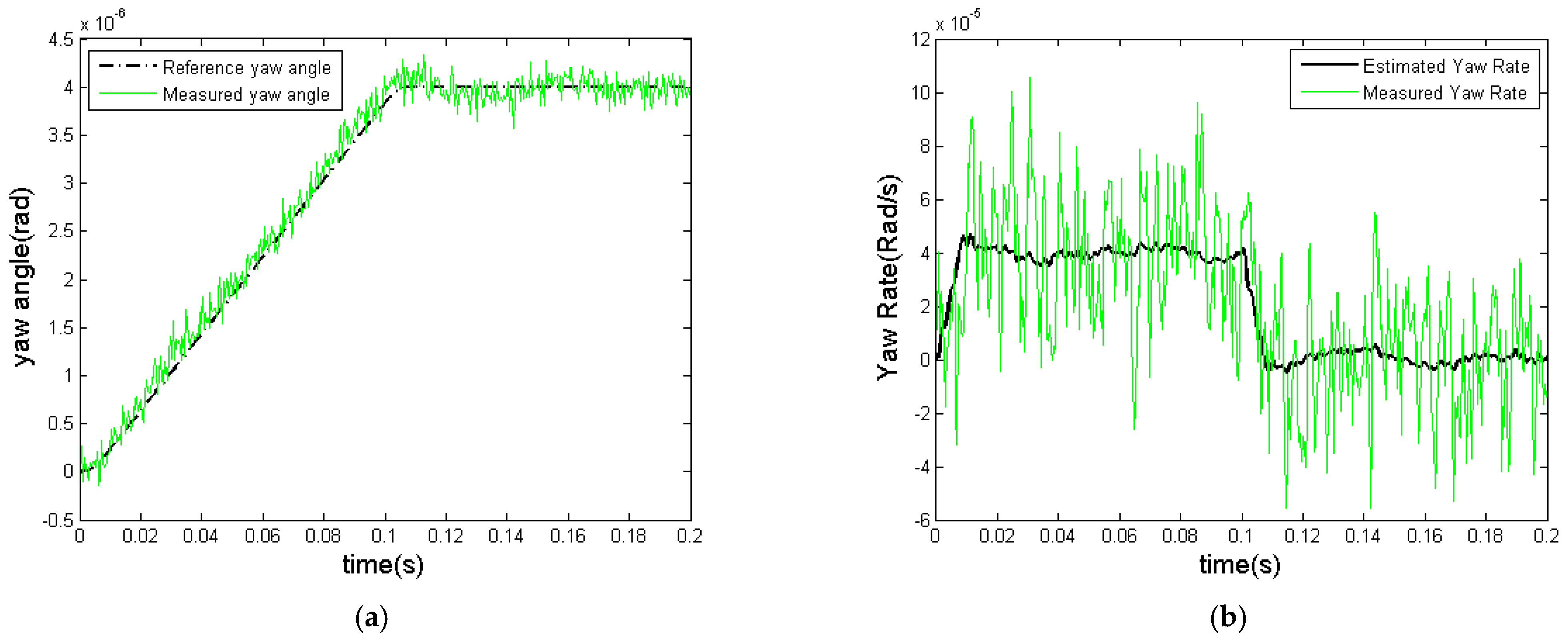
Implementation in the Presence of Position Measurement Noise

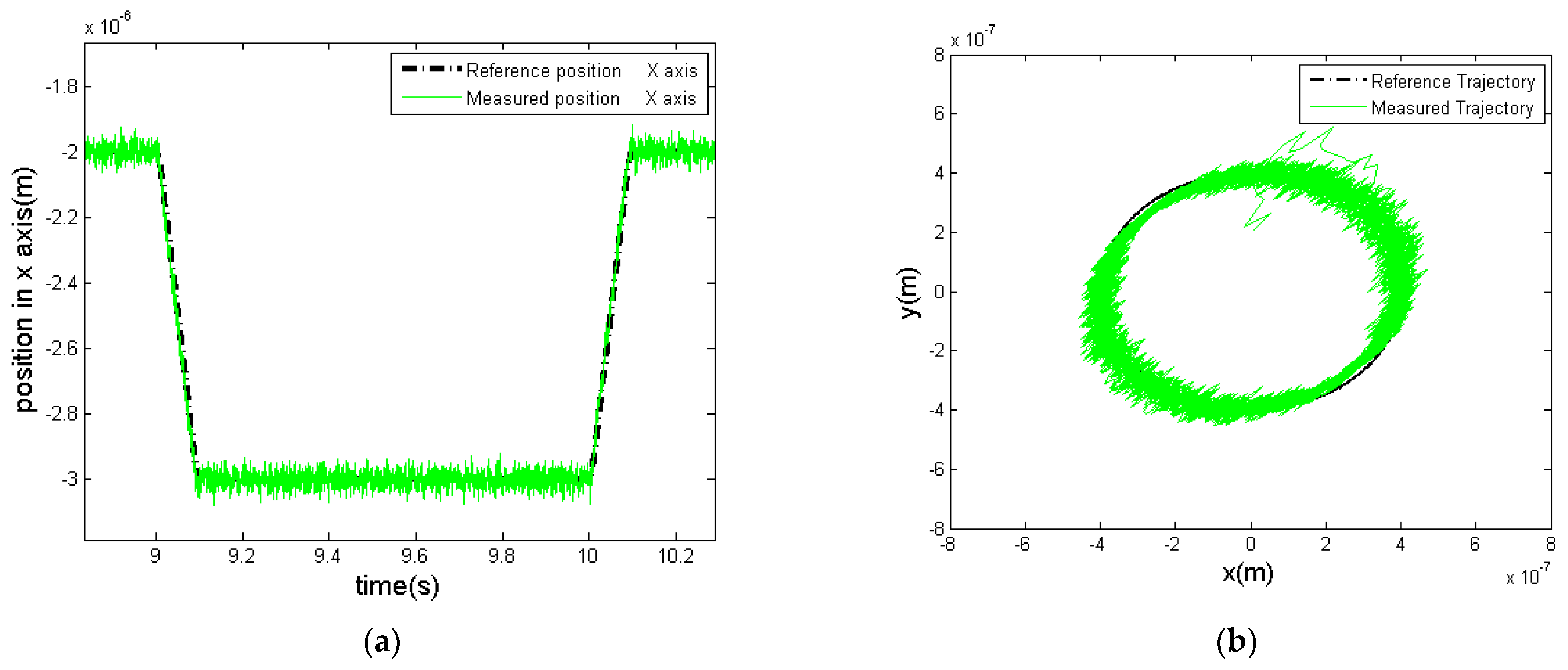
Although the proposed velocity observer is proven stable, its performance is sensitive to position measurement noise in a real-time implementation. In our set-up, the RMS measurement noise in the capacitive sensing system is estimated at ±60 nm at the high-sensitivity measurement setting. A second-order digital low-pass filter H(z) with a linear phase was used for each axis (Figure 2b) to filter position readings from the capacitive sensors; the cut-off frequency was chosen as 120 Hz since this is the (−3 dB) sensor bandwidth:

$$H\left(z\right)={\lambda }_3/\left(1+{\lambda }_1{z}^{-1}+{\lambda }_2{z}^{-2}\right)$$

(20)

The linear phase in the filter’s pass band guarantees that the position waveform measured by the capacitive sensor will not be distorted, as needed for high-precision positioning and tracking. Figure 4a,b show the frequency response of the proposed filter.

The observer gains and filter coefficients used in the low-pass filter are shown in

Table 2. Nonlinear passive observer (NPO) and low-pass filter (LPF) parameters.

NPO	LPF
$$\begin{gathered} {\mathbf{D}}_0=diag\left(100,100,100,100,100,100\right) \\ {\mathbf{A}}_0=diag\left({10}^4,{10}^4,{10}^4,{10}^4,{10}^4,{10}^4\right) \end{gathered}$$	$$\begin{gathered} {\lambda }_1=0.79954 \\ {\lambda }_2=0.65902 \\ {\lambda }_3=0.05994 \end{gathered}$$

.

3. Results

The capability of synchronized high-precision linear and rotary motions is crucial for applications such as lens manufacturing, mask alignment, and wafer alignment in semiconductor manufacturing. Performance of the proposed estimation method in x-y-θ motion is shown in Figure 5, Figure 6 and Figure 7. In Figure 5a and Figure 6a, the positioning stage was commanded to move 500 nm and 250 nm in the direction of the x- and y-axis, respectively, while in Figure 7a it was commanded to rotate about the y-axis by 4 μrad. The corresponding velocity estimations in each case, using the proposed nonlinear passive observer, are shown in Figure 5b, Figure 6b, and Figure 7b, respectively, demonstrating adequate multi-axis motion estimation performances compared to the measured velocity. The trajectories shown are simultaneously (multi-axis synchronized motion).

Estimation of Reciprocating Motion and Synchronous Motion

Reciprocal motion is commonly used in micromachining processes where the velocity of the cutting tool needs to change direction periodically. Figure 8a shows the position of the moving stage after being commanded to move back 1 μm along the x-direction, hold position, and then return to the original location. The corresponding velocity estimations, in both the negative and positive x-direction, are shown in Figure 9a,b, further illustrating the performance of the proposed observer. The reference acceleration was set as constant: 1 mm/s² for acceleration and −1 mm/s² for deceleration. The reference velocities commanded by the path-planning algorithm are trapezoidal curves with the flat part being 11.5 μm/s and −11.5 μm/s, respectively.

Execution of circular trajectories requires synchronization of two axes of motion, as used in direct-write nanopatterning and nanomachining processes. To test performance in this kind of maneuver, the positioning stage was commanded to follow a circular path with a radius of 400 nm, as shown in Figure 8b. Figure 10a,b show the corresponding velocity estimation results in the x- and y-axis, respectively, illustrating the proposed observer’s ability to estimate velocity in the presence of a continuous change in direction.

4. Discussion

In high-precision positioning applications, a state estimator is needed to distinguish true motion from measurement noise. In linear systems, state estimation from noisy measurements is possible using a Kalman filter; in nonlinear systems, an extended Kalman filter can be used but only local stability is guaranteed.

Early observer design for dynamic positioning focused on linear optimal observer design from linearized equations of motion. Due to the lack of global stability, the research shifted to nonlinear observer design, with the disadvantage that optimality is not guaranteed.

Passivity has been of interest in the analysis of nonlinear systems: by introducing the notions of storage function and supply rate, less conservativeness in the demonstration of robust stability is needed. Passivity can guarantee the existence of a high-gain robust observer in a class of nonlinear uncertain systems; but observer design based on passivity has rarely been discussed.

Recent efforts have used passivity to demonstrate robustness and the global exponential stability of nonlinear observers. The proposed nonlinear passive observer (NPO) is designed directly from the free-body dynamics of the motion stage with no assumptions of linearity or decoupling, based on a Lyapunov stability approach. The proposed NPO is proved to achieve global stability, in contrast to local stability provided by conventional extended Kalman filters.

Several experiments were performed to demonstrate the performance of the proposed NPO. First, an x-y-θ alignment motion demonstrated the multi-axis motion estimation capability of the NPO. Then, a reciprocating motion was used to illustrate that the NPO is able to estimate velocity in the presence of alternating changes in direction. Lastly, a trajectory that required synchronous two-axis motion was used to illustrate the NPO’s ability to estimate multi-axial velocity in the presence of a continuous change in direction. The experimental results illustrate that the proposed NPO performs very well in providing reliable velocity estimation in high-precision multi-axis motion control applications.

5. Conclusions

A nonlinear passive observer design has been proposed to estimate the multi-axis velocity of the coupled six-axis free-body dynamics of a levitated high-precision magnetically suspended stage. The work from [18] was extended to propose a modified nonlinear passive observer that can provide six-axis motion estimation for high-precision motion control based on a Lyapunov method. Compared to a conventional Kalman filter, a smaller number of tuning parameters is needed since no linearization of the kinematic equations is necessary, and global stability is achieved.

Coupling effects between axes degrade positioning performance when approximated linear decoupled dynamics are assumed. The proposed nonlinear passive observer is an innovation that can be used in support of synchronized multi-axis motion control in high-precision applications such as semiconductor manufacturing.

References

1. Gu, J.; Kim, W.-J.; Verma, S. Nanoscale motion control with a compact minimum-actuator magnetic levitator. ASME J. Dyn. Syst. Meas. Control 2005, 127, 433–442. [Google Scholar] [CrossRef]
2. Kim, W.-J.; Trumper, D.L.; Lang, J.H. Modeling and vector control of planar magnetic levitator. IEEE Trans. Ind. Appl. 1998, 34, 1254–1262. [Google Scholar]
3. Shakir, H.; Kim, W.-J. Nanoscale path planning and motion control with maglev positioners. IEEE/ASME Trans. Mechatron. 2006, 11, 625–633. [Google Scholar] [CrossRef]
4. Shan, X.; Kuo, S.K.; Zhang, J.; Menq, C.H. Ultra precision motion control of a multiple degrees of magnetic suspension system. IEEE/ASME Trans. Mechatron. 2002, 7, 67–78. [Google Scholar] [CrossRef]
5. Kuo, S.-K.; Menq, C.-H. Modeling and control of a six-axis precision motion control stage. IEEE/ASME Trans. Mechatron. February 2005, 10, 50–59. [Google Scholar] [CrossRef]
6. Tai, T.-L.; Chen, J.-S. Discrete-time sliding-mode controller for dual-stage systems—A hierarchical approach. Mechatronics 2005, 15, 949–967. [Google Scholar] [CrossRef]
7. Kim, H.M.; Park, S.H.; Han, S.I. Precise friction control for the nonlinear friction system using the friction state observer and sliding mode control with recurrent fuzzy neural networks. Mechatronics 2009, 19, 805–815. [Google Scholar] [CrossRef]
8. Ludwick, S.J.; Trumper, D. Modeling and control of a six degree-of-freedom magnetic/fluidic motion control stage. IEEE Trans. Control Syst. Technol. 1996, 4, 553–564. [Google Scholar] [CrossRef]
9. Hirvonen, M.; Pyrhonen, O.; Handroos, H. Adaptive nonlinear velocity controller for a flexible mechanism of a linear motor. Mechatronics 2006, 16, 279–290. [Google Scholar] [CrossRef]
10. Onodera, R.; Mimura, N. Measurement of vehicle motion using a new 6-DOF motion sensor system–Angular velocity estimation with Kalman filter using motion characteristic of a vehicle. J. Robot. Mechatron. 2008, 20, 116–124. [Google Scholar] [CrossRef]
11. Alasty, A.; Shabani, R. Nonlinear parametric identification of magnetic bearings. Mechatronics 2006, 16, 451–459. [Google Scholar] [CrossRef]
12. Dini, P.; Saponara, S. Design of an Observer-Based Architecture and Non-Linear Control Algorithm for Cogging Torque Reduction in Synchronous Motors. Energies 2020, 13, 2077. [Google Scholar] [CrossRef]
13. Dini, P.; Saponara, S. Model-Based Design of an Improved Electric Drive Controller for High-Precision Applications Based on Feedback Linearization Technique. Electronics 2021, 10, 2954. [Google Scholar] [CrossRef]
14. Slotine, J.J.; Hedrick, J.K.; Misawa, E.A. On sliding observers for nonlinear systems. J. Dyn. Syst. Meas. Control 1987, 109, 245–252. [Google Scholar] [CrossRef]
15. Lu, Y.-S.; Cheng, C.-M.; Cheng, C.-H. Non-overshooting PI control of variable-speed motor drives with sliding perturbation observers. Mechatronics 2005, 15, 1143–1158. [Google Scholar] [CrossRef]
16. Emaru, T.; Imagawa, K.; Hoshino, Y.; Kobayashi, Y. Velocity and acceleration estimation by a nonlinear filter based on sliding mode and application to control system. J. Robot. Mechatron. 2009, 21, 590–596. [Google Scholar] [CrossRef]
17. Mokhtari, A.; Benallegue, A.; Belaidi, A. Polynomial Linear Quadratic Gaussian and sliding mode observer for a quadrotor unmanned aerial vehicle. J. Robot. Mechatron. 2005, 17, 483–495. [Google Scholar] [CrossRef]
18. Loria, A.; Fossen, T.I.; Panteley, E. A separation principle for dynamic positioning of ships: Theoretical and experimental results. IEEE Trans. Control Syst. Technol. 2000, 8, 332–343. [Google Scholar] [CrossRef]
19. Dabroom, A.M.; Khalil, H.K. Discrete-time implementation of high-gain observers for numerical differentiation. Int. J. Control 1999, 72, 1523–1537. [Google Scholar] [CrossRef]
20. Khalil, H.K. Nonlinear Systems, 3rd ed.; Prentice Hall: Upper Saddle River, NJ, USA, 2002. [Google Scholar]
21. Atassi, A.N.; Khalil, H.K. A separation principle for the stabilization of a class of nonlinear systems. IEEE Trans. Autom. Control 1999, 44, 1672–1687. [Google Scholar] [CrossRef]
22. Nazrulla, M.S.; Khalil, H.K. Robust stabilization of non-minimum phase nonlinear systems using extended high gain observers. IEEE Trans. Autom. Control 2011, 56, 802–813. [Google Scholar] [CrossRef]
23. Bando, M.; Ichikawa, A. Adaptive regulation of nonlinear systems by output feedback. J. Robot. Mechatron. 2008, 20, 719–725. [Google Scholar] [CrossRef]
24. Willems, J.C. Dissipative dynamical systems—Part I: General theory. Arch. Ration. Mech. Anal. 1972, 45, 321–351. [Google Scholar] [CrossRef]
25. Willems, J.C. Dissipative dynamical systems—Part II: Linear systems with quadratic supply rates. Arch. Ration. Mech. Anal. 1972, 45, 352–393. [Google Scholar] [CrossRef]
26. Liu, W.; Wang, Z.; Chen, G.; Sheng, L. Passivity-based observer design and robust output feedback control for nonlinear uncertain systems. In Proceedings of the 9th Asian Control Conference, Istanbul, Turkey, 23–26 June 2013; pp. 1–6. [Google Scholar] [CrossRef]
27. Yang, X.; Liu, R.; Guo, L. A Robust Sliding Mode Observer for Dynamic Positioning System. In Proceedings of the 2019 IEEE 3rd Advanced Information Management, Communicates, Electronic and Automation Control Conference, Chongqing, China, 11–13 October 2019; pp. 85–90. [Google Scholar] [CrossRef]
28. Xie, D.; Jia, B.; Ren, Y. Control System Design for Dynamic Positioning Ships Using Nonlinear Passive Observer Backstepping. In Proceedings of the 2018 Chinese Automation Congress, Xi’an, China, 30 November–2 December 2018; pp. 4221–4226. [Google Scholar] [CrossRef]
29. Alvarez-Salas, R.; Gallegos, M.; Moreno, J.; Espinosa-Perez, G. A passive speed observer for induction motor. In Proceedings of the 6th International Conference on Electrical Engineering, Computing Science and Automatic Control, Toluca, Mexico, 10–13 January 2009; pp. 1–6. [Google Scholar] [CrossRef]
30. Almeida, J.; Loukianov, A.; Cañedo Castañeda, J. Passive observer-based control of synchronous generator. In Proceedings of the 2016 IEEE International Meeting on Power, Electronics and Computing, Ixtapa, Mexico, 9–11 November 2016; pp. 1–6. [Google Scholar] [CrossRef]
31. Snijders, J.; van der Woude, J.; Westhuis, J. Nonlinear Observer Design for Dynamic Positioning. In Proceedings of the Marine Technology Society Dynamic Positioning Conference, Houston, TX, USA, 15–16 November 2005. [Google Scholar]
32. Liu, R.; Yang, X.; Jia, Y. Design of Nonlinear Observer for Ship Dynamic Positioning System. In Proceedings of the 2019 IEEE 3rd Information Technology, Networking, Electronic and Automation Control Conference, Chengdu, China, 15–17 March 2019; pp. 1339–1342. [Google Scholar] [CrossRef]
33. Lin, X.; Li, H.; Liang, K.; Jiao, Y. Nonlinear passive robust observer design for a DP system based on ACA. In Proceedings of the 36th Chinese Control Conference, Dalian, China, 26–28 July 2017; pp. 474–481. [Google Scholar] [CrossRef]
34. Xia, G.; Shao, X. Sliding mode control based on passive nonlinear observer for dynamic positioning vessels. In Proceedings of the 2011 International Conference on Mechatronic Science, Electric Engineering and Computer, Jilin, China, 19–22 August 2011; pp. 2156–2159. [Google Scholar] [CrossRef]
35. Fossen, T.; Strand, J. Passive Nonlinear Observer Design for Ships Using Lyapunov Methods: Full-Scale Experiments with a Supply Vessel. Automatica 1999, 35, 3–28. [Google Scholar] [CrossRef]
36. Xie, D.; Han, X.; Jia, B.; Liu, Y.; Zheng, S. Research on improved PID Dynamic Positioning System Based on Nonlinear Observer. In Proceedings of the 2018 Chinese Automation Congress, Xi’an, China, 30 November–2 December 2018; pp. 698–702. [Google Scholar] [CrossRef]
37. Tong, X.; Chen, M.; Yang, F. Passive and Explicit Attitude and Gyro-Bias Observers Using Inertial Measurements. IEEE Trans. Ind. Electron. 2021, 68, 8942–8952. [Google Scholar] [CrossRef]
38. Li, D.; Gutierrez, H. Quasi-sliding mode control of a high precision hybrid magnetic suspension actuator. J. Robot. Mechatron. 2013, 25, 192–200. [Google Scholar] [CrossRef]
39. Li, D. Modeling and Control of a High Precision 6-DOF Maglev Positioning Stage with Large Range of Travel. Ph.D. Dissertation, Florida Institute of Technology, Melbourne, FL, USA, December 2008. [Google Scholar]
40. Wang, Y.; Pan, T.; Wong, D.; Tan, F. An Extended State Observer-Based Run to Run Control for Semiconductor Manufacturing Processes. IEEE Trans. Semicond. Manuf. 2019, 32, 154–162. [Google Scholar] [CrossRef]
41. Lee, A.; Pan, Y.; Hsieh, M. Output Disturbance Observer Structure Applied to Run-to-Run Control for Semiconductor Manufacturing. IEEE Trans. Semicond. Manuf. 2011, 24, 27–43. [Google Scholar] [CrossRef]
42. Tsai, M.; Peng, C. Sliding Mode Observer Based Multi-Layer Metal Plates Core Temperature On-Line Estimation for Semiconductor Intelligence Manufacturing. IEEE Access 2020, 8, 194561–194574. [Google Scholar] [CrossRef]
43. Li, D.; Gutierrez, H. Precise motion control of a hybrid magnetic suspension actuator with large travel. In Proceedings of the 34th IEEE Annual Conference on Industrial Electronics, IECON 2008, Orlando, FL, USA, 10–13 November 2008; pp. 2661–2666. [Google Scholar]
44. Li, D.; Gutierrez, H. Observer-based sliding mode control of a 6-DOF precision maglev positioning stage. In Proceedings of the 34th IEEE Annual Conference on Industrial Electronics, IECON 2008, Orlando, FL, USA, 10–13 November 2008; pp. 2562–2567. [Google Scholar]
45. Hu, T.; Kim, W.-J. Extended range six DOF high-precision positioner for wafer processing. IEEE/ASME Trans. Mechatron. 2006, 11, 682–689. [Google Scholar] [CrossRef]
46. Jung, K.S.; Lee, S.H. Contact-free planar stage using linear induction principle. Mechatronics 2010, 20, 518–526. [Google Scholar] [CrossRef]
47. Estevez, P.; Mulder, A.; Munnig Schmidt, R.H. 6-DoF miniature maglev positioning stage for application in haptic micro-manipulation. Mechatronics 2012, 22, 1015–1022. [Google Scholar] [CrossRef]
48. Jung, K.S.; Baek, Y.S. Development of a novel maglev positioner with self-stabilizing property. Mechatronics 2002, 12, 771–790. [Google Scholar] [CrossRef]
Figure 1. Multi-axis high-precision motion control stage, (a) stationary and moving parts, (b) moving part showing permanent magnet stacks, actuator target areas, and sensor target areas.
Machines 12 00376 g001
Figure 2. Multi-axis high-precision motion control stage, (a) moving part and base showing actuator and sensor locations, (b) implementation showing axes of motion and axes of rotation.
Machines 12 00376 g002
Figure 3. Implementation and testing of the proposed approach. (a) The real-time control platform based on TI-6701 DSP; (b) the low-pass filter for implementation of a nonlinear passive observer (NPO).
Machines 12 00376 g003
Figure 4. Frequency response of the H(z) digital low-pass filter (a). Frequency response over the entire design range; (b) frequency response in the application’s pass band.
Machines 12 00376 g004
Figure 5. Step response to 500 nm command on x-axis, (a) position response, and (b) velocity response and velocity estimation on x-axis.
Machines 12 00376 g005
Figure 6. Step response to 250 nm command on y-axis, (a) position response, and (b) velocity response and velocity estimation on y-axis.
Machines 12 00376 g006
Figure 7. Step response to 4 μrad command on θ-axis, (a) angular position response (yaw), and (b) velocity response and velocity estimation on yaw-axis.
Machines 12 00376 g007
Figure 8. (a) Reciprocating motion on x-axis; (b) synchronized circular trajectory in XY plane.
Machines 12 00376 g008
Figure 9. Estimator performance during reciprocating motion on x-axis; (a) estimation of positive velocity; (b) estimation of negative velocity.
Machines 12 00376 g009
Figure 10. Estimator performance in synchronized trajectory in the XY plane, (a) velocity estimation on the x-axis during circular motion; (b) velocity estimation on the y-axis during circular motion.
Machines 12 00376 g010