A Review of Time-Series Forecasting Algorithms for Industrial Manufacturing Systems

Abstract

Time-series forecasting is crucial in the efficient operation and decision-making processes of various industrial systems. Accurately predicting future trends is essential for optimizing resources, production scheduling, and overall system performance. This comprehensive review examines time-series forecasting models and their applications across diverse industries. We discuss the fundamental principles, strengths, and weaknesses of traditional statistical methods such as Autoregressive Integrated Moving Average (ARIMA) and Exponential Smoothing (ES), which are widely used due to their simplicity and interpretability. However, these models often struggle with the complex, non-linear, and high-dimensional data commonly found in industrial systems. To address these challenges, we explore Machine Learning techniques, including Support Vector Machine (SVM) and Artificial Neural Network (ANN). These models offer more flexibility and adaptability, often outperforming traditional statistical methods. Furthermore, we investigate the potential of hybrid models, which combine the strengths of different methods to achieve improved prediction performance. These hybrid models result in more accurate and robust forecasts. Finally, we discuss the potential of newly developed generative models such as Generative Adversarial Network (GAN) for time-series forecasting. This review emphasizes the importance of carefully selecting the appropriate model based on specific industry requirements, data characteristics, and forecasting objectives.

1. Introduction

The advent of Artificial Intelligence (AI) has ushered in a transformative era for manufacturing systems, catalyzing advancements in operational efficiency, quality assurance, and predictive maintenance. Machine Learning (ML) algorithms, along with conventional statistical models, have become instrumental in deciphering complex patterns within voluminous datasets, thereby facilitating more informed decision-making processes in manufacturing environments [1]. For instance, predictive maintenance, powered by ML algorithms, has enabled the proactive identification of potential equipment failures, significantly reducing downtime and associated costs [2]. Manufacturing systems, when supported by AI algorithms, enhance production quality by autonomously detecting defects, thus ensuring product consistency and reducing waste [3]. The integration of these intelligent models not only ensures the robustness of manufacturing systems but also propels them toward a future where data-driven insights pave the way for innovative, sustainable, and efficient production mechanisms.

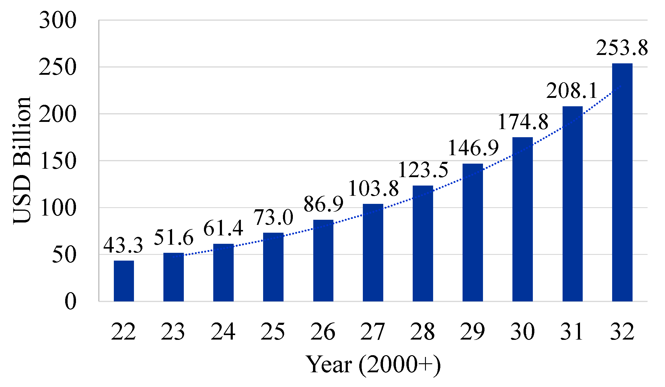
1.1. Significance of Time-Series Forecasting in Industrial Manufacturing Systems

Manufacturing systems inherently generate time-series data, which are a set of observations recorded at consistent time intervals, which includes the dynamic and temporal variations in the manufacturing processes [4]. This type of data can include a variety of variables such as production rates, machine utilization, and quality metrics and is pivotal for capturing the temporal dependencies and underlying patterns within the manufacturing operations [5]. The significance of time-series data in forecasting is paramount, and it enables consumers to optimize their resources, improve operational efficiency, and implement predictive maintenance strategies [6]. Using the historical patterns embedded within time-series data, forecasting models can anticipate future demands and challenges for manufacturing systems, ensuring robust, sustainable, and efficient production cycles in an increasingly competitive industrial landscape.

The intricacies of modern manufacturing processes, characterized by complex supply chains, variable demand, and the need for precision, further underscore the importance of accurate time-series forecasting. For instance, predictive maintenance by forecasting potential failures can not only ensure uninterrupted production but also extend the lifespan of machinery, leading to significant cost savings [6]. Furthermore, in an era where just-in-time production and lean manufacturing principles are paramount, the ability to accurately forecast demand and supply dynamics becomes indispensable. It aids in reducing inventory costs, improving cash flow, and ensuring timely delivery to customers, thereby enhancing overall customer satisfaction [7].

The manufacturing industry has been heavily investing in the development of AI systems for optimizing their production processes. In 2023, the AI market in the manufacturing sector was valued at USD 3.8 billion with an expected Compound Annual Growth Rate (CAGR) of 45%, and it is estimated to reach USD 156.1 billion by 2033 [8]. The demand for predictive maintenance systems is expected to have a rapid revenue rise, already being used across various end-use industries. Various sensors and cameras are placed on the equipment on the production floors to gather data and analyze operational parameters such as temperature, vibrations, and wear of the moving parts. The AI algorithms analyze these data to train the predictive models and provide insights to the manufacturer. These are the driving factors for the increased demand for AI in manufacturing, which is reflected in the increasing revenue trend. The projected growth of AI systems revenue in the manufacturing sector is shown in Figure 1.

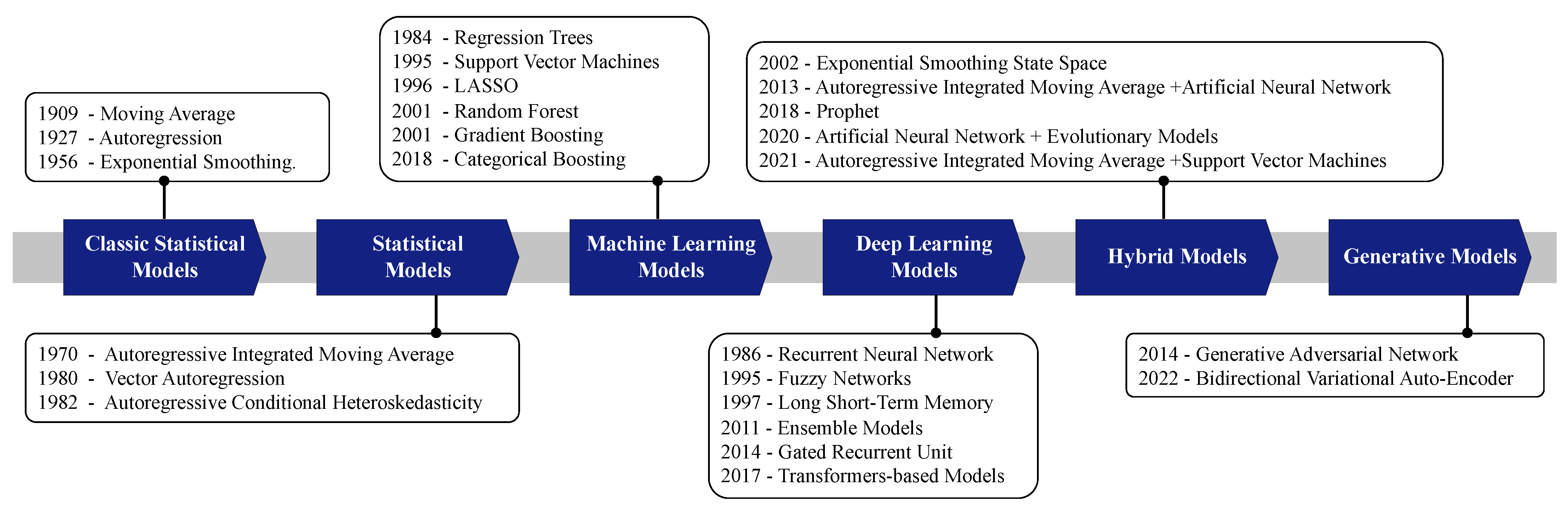
1.2. Evolution of Time-Series Forecasting Algorithms

The chronological progression of time-series forecasting methodologies exhibits a series of statistical and algorithmic innovations. Initial approaches were predominantly statistical, with simple models such as the Moving Average (MA), Autoregression (AR), and ES providing a foundational framework for early time-dependent data analysis. These classical models encapsulated the essence of time-series forecasting, enabling practitioners to identify patterns and trends within temporal datasets across multiple disciplines.

Advancements in the latter 20th century introduced enhanced versions of traditional models, including ARIMA, Vector Autoregression (VAR), and Autoregressive Conditional Heteroskedasticity (ARCH). Among these, the ARIMA model has sustained its prominence within the forecasting domain and is often used with emerging ML and DL techniques. Concurrently, the field of ML, which has roots extending to the late 18th century, became more popular as new variations kept developing in the late 20th century, setting the stage for contemporary applications in time-series forecasting. While DL models are a subset of ML, their complexity and wide variety of specialized architectures, such as Recurrent Neural Network (RNN), Long Short-Term Memory (LSTM), and Gated Recurrent Unit (GRU), justify them being presented as a distinct category. The timeline is shown in Figure 2, and further details are explained in Table 1. These classes have been selected to provide a clear and organized view of the evolution of models in the context of time-series forecasting, including classic statistical models, statistical models, Machine Learning models, Deep Learning models, hybrid models, and generative models. This classification helps us to understand the chronological progression and distinct characteristics of each category.

Classic statistical models laid the groundwork for time-series forecasting. These were followed by more sophisticated statistical models, which incorporated more advanced statistical techniques. ML models brought a new dimension, with advanced algorithms focusing on predictive accuracy through data-driven approaches. DL models, despite being a subset of ML, are highlighted separately due to their unique architectures and transformative influence on the field, making them a focal point of modern research and applications. Hybrid models represent a combination of one or more fundamental models to leverage the strengths of each component. These models blend different methodologies to improve forecasting accuracy and robustness. For example, integrating an ES model with an ANN model improves the capability of the model to capture linear and especially non-linear patterns in time-series datasets. Although ES and ANN can both compute linear and non-linear data features, ANN alone has limited capacity to handle linear data as accurately as non-linear patterns [10]. Generative models, such as GANs, have introduced innovative approaches to time-series forecasting by focusing on the generation and understanding of complex data distributions. These models are particularly valuable in scenarios where simulating potential future data points is crucial.

Table 1. Chronological list of developments in time-series forecasting field.

Category	Method	Year	Origin Paper	Application Paper
Classical Statistical Methods (Before 1970)	MA	1909	[11]	[12,13,14,15]
	AR	1927	[16]	[12,17,18]
	ES	1956	[19]	[20,21,22,23]
Classical Statistical Methods (1970s to 2000s)	ARIMA	1970	[24]	[12,25,26,27,28,29,30,31,32,33,34,35]
	Seasonal Autoregressive Integrated Moving Average (SARIMA)	1970	[24]	[25,36,37,38,39,40]
	Vector Autoregression (VAR)	1980	[41]	[42]
	Autoregressive Conditional Heteroskedasticity	1982	[35]	[43]
	Generalized AutoRegressive Conditional Heteroskedasticity (GARCH)	1986	[44]	[45]
	State-Space Models	1994	[46]	[47]
Machine Learning Methods (1960s to 2010s)	Decision Trees	1963	[48]	[49]
	Regression Trees	1984	[50]	[49,51]
	SVM	1995	[52]	[53,54,55,56,57,58,59]
	LASSO Regression	1996	[60]	[61,62,63]
	k-Nearest Neighbors (KNN)	Various	[64]	[6,65,66,67]
	Random Forests	2001	[68]	[59,69,70,71,72]
	Gradient Boosting Machines	2001	[73]	[74,75,76,77,78]
	Categorical Boosting	2018	[79]	[80]
	Prophet	2018	[81]	[82,83,84,85,86]
Deep Learning Methods (1950s to 2010s)	ANN	1958	[87]	[12,34,88,89,90,91,92]
	Recurrent Neural Network (RNN)	1986	[93]	[94,95,96]
	Bayesian Models	1995	[97]	[98]
	Fuzzy Networks	1995	[99]	[100,101,102,103,104]
	Long Short-Term Memory (LSTM)	1997	[105]	[84,106,107]
	Ensemble Models	2011	[108]	[109]
	Gated Recurrent Unit (GRU)	2014	[110]	[111]
	Transformer-based Models	2017	[112]	[113]
Hybrid Models (2000s to 2020s)	Exponential Smoothing State-Space Model (ETS)	2002	[114]	[114,115,116]
	ARIMA + ANN	2013	[29]	[29,90,117,118]
	ANN + Evolutionary models	2020	[119]	[119,120,121,122]
	ARIMA + SVM	2021	[123]	[123,124,125]
Generative Models (2010s to 2020s)	GAN	2014	[126]	[127,128]
	Bidirectional Variational Auto-Encoder	2022	[129]	[130,131]

Table 1. Chronological list of developments in time-series forecasting field.

Category	Method	Year	Origin Paper	Application Paper
Classical Statistical Methods (Before 1970)	MA	1909	[11]	[12,13,14,15]
	AR	1927	[16]	[12,17,18]
	ES	1956	[19]	[20,21,22,23]
Classical Statistical Methods (1970s to 2000s)	ARIMA	1970	[24]	[12,25,26,27,28,29,30,31,32,33,34,35]
	Seasonal Autoregressive Integrated Moving Average (SARIMA)	1970	[24]	[25,36,37,38,39,40]
	Vector Autoregression (VAR)	1980	[41]	[42]
	Autoregressive Conditional Heteroskedasticity	1982	[35]	[43]
	Generalized AutoRegressive Conditional Heteroskedasticity (GARCH)	1986	[44]	[45]
	State-Space Models	1994	[46]	[47]
Machine Learning Methods (1960s to 2010s)	Decision Trees	1963	[48]	[49]
	Regression Trees	1984	[50]	[49,51]
	SVM	1995	[52]	[53,54,55,56,57,58,59]
	LASSO Regression	1996	[60]	[61,62,63]
	k-Nearest Neighbors (KNN)	Various	[64]	[6,65,66,67]
	Random Forests	2001	[68]	[59,69,70,71,72]
	Gradient Boosting Machines	2001	[73]	[74,75,76,77,78]
	Categorical Boosting	2018	[79]	[80]
	Prophet	2018	[81]	[82,83,84,85,86]
Deep Learning Methods (1950s to 2010s)	ANN	1958	[87]	[12,34,88,89,90,91,92]
	Recurrent Neural Network (RNN)	1986	[93]	[94,95,96]
	Bayesian Models	1995	[97]	[98]
	Fuzzy Networks	1995	[99]	[100,101,102,103,104]
	Long Short-Term Memory (LSTM)	1997	[105]	[84,106,107]
	Ensemble Models	2011	[108]	[109]
	Gated Recurrent Unit (GRU)	2014	[110]	[111]
	Transformer-based Models	2017	[112]	[113]
Hybrid Models (2000s to 2020s)	Exponential Smoothing State-Space Model (ETS)	2002	[114]	[114,115,116]
	ARIMA + ANN	2013	[29]	[29,90,117,118]
	ANN + Evolutionary models	2020	[119]	[119,120,121,122]
	ARIMA + SVM	2021	[123]	[123,124,125]
Generative Models (2010s to 2020s)	GAN	2014	[126]	[127,128]
	Bidirectional Variational Auto-Encoder	2022	[129]	[130,131]

1.3. Objectives of the Review

Statistical models have been considered for time-series forecasting since the 1970s, especially the Box–Jenkins methods [24]. With the development of ML and its variations, many models have been developed, which are proven to outperform the classical statistical models. However, methods based on neural networks are currently achieving better results, and new model architectures are focused on research that provides flexibility with the changing patterns in the data. This paper aims to provide a comprehensive understanding of popular time-series forecasting models and their applications and performance in manufacturing systems. Furthermore, research gaps have been identified in the literature to inspire and direct the research in this domain.

Other survey papers have been published recently that provide an overview of time-series forecasting models. Torres et al. [132] reviewed the Deep Learning (DL) models for forecasting, including the mathematical structure of these models. A similar study was presented by Lara-Benitez et al. [133], which provided an experimental review of Deep Learning models. Another comprehensive study was performed by Deb et al. [6], where the authors analyzed the time-series forecasting models for building energy consumption. Masini et al. [134] have recently published a survey about the advances in ML models for time-series forecasting and provided the mathematical details of the models. Ensafi et al. [84] have published the experimental comparison of some Machine Learning models for seasonal item sales. Gasparin et al. [135] have recently published a use case of electric load forecasting using Deep Learning algorithms and have compared their performance.

There are various forecasting models available for time-series data, such as image-, audio-, and text-based datasets, as well as for time-series data, including financial, weather, and health systems datasets. Despite the emergence of several recent publications that analyze various ML models for time-series forecasting, a gap exists in the literature regarding a comprehensive analysis of these models, specifically within the context of manufacturing systems, as demonstrated in Figure 3. While these existing papers provide valuable insights into the comparative performance of these models in generic settings or for other types of time-series data, such as sales and finance datasets, they often do not delve into the unique challenges and considerations intrinsic to manufacturing environments, such as constraints on data availability, missing data, features extraction, and model robustness and reliability. Manufacturing systems, with their inherent complexities and multifaceted variables, necessitate a detailed exploration that not only includes models’ predictive accuracy but also encompasses a broader spectrum of factors pivotal for practical implementation. This paper, therefore, seeks to bridge this gap by undertaking a comprehensive analysis of time-series forecasting models in manufacturing systems. It aims to navigate the challenges posed by manufacturing data and operational contexts, thereby providing a holistic evaluation that aligns more closely with the real-world applicability and efficacy of these forecasting models in manufacturing scenarios and that presents their advantages and challenges. The objectives of this review paper are:

• To provide a comprehensive review of the classical statistical, ML, DL, and hybrid models used in manufacturing systems.
• To conduct a comparative study encompassing both the qualitative and quantitative dimensions of these methods.
• To explore the different hybrid model combinations, evaluating their effectiveness and performance.

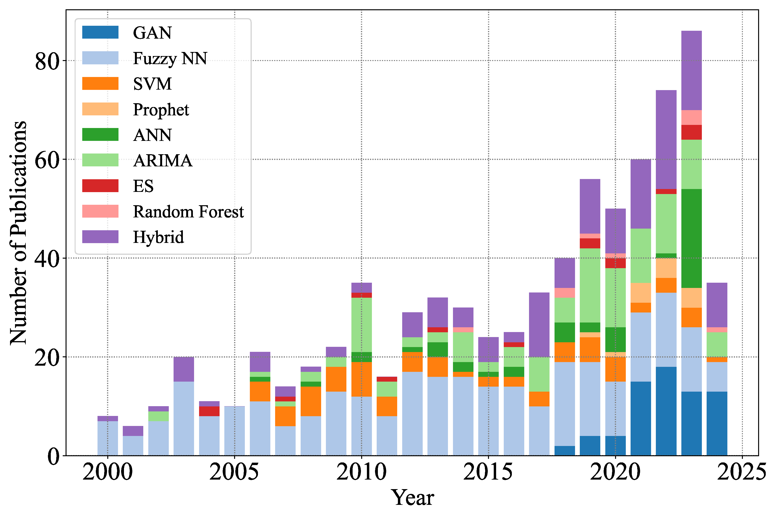
1.4. Summary of Reviewed Papers

In this comprehensive review of the literature on time-series forecasting, various approaches and techniques were employed to address various challenges and applications. The reviewed papers spanned from traditional statistical methods, such as ARIMA, MA, and ES, to more advanced Machine Learning and Deep Learning-based models, including the Feed-Forward Neural Network (FFNN), Recurrent Neural Network (RNN), decision trees, and GAN. The reviewed literature also highlighted the importance of addressing seasonality, trend components, and multivariate relationships to improve forecasting accuracy. Additionally, it was found that hybrid models have gained significant attention in recent years as researchers aim to combine the strengths of multiple models to enhance predictive performance. Overall, the body of literature on time-series forecasting showcases the continuous development and refinement of methods, as well as the increasing importance of accurate predictions across a wide array of disciplines and industries. The number of publications in the domain of time-series forecasting is illustrated in Figure 4, where the number of publications for each model is plotted against the years from 2000 to 2024. These statistics were collected from Google Scholar. The structure of the review paper is as follows: first, an overview of time-series data definitions and subdivisions is provided in Section 2, followed by a review of the most common time-series forecasting algorithms, along with the chronological order of the development of these models. Later, in Section 3, the details of these algorithms, including their mathematical structure and their applications in the manufacturing sector, with the help of published used cases, have been provided. For each paper reviewed, emphasis is given to the study’s objective, and the models’ performances are usually measured in Mean Absolute Percentage Error (MAPE). A detailed discussion of the reviewed algorithms and the hybrid models is provided in Section 4. A detailed analysis and comparison of some of the hybrid models are also presented in this section, including the advantages and disadvantages of some of the independent models used to give researchers a direction for hybrid frameworks. The existing challenges and future research directions from this review are provided in Section 5. Finally, the concluding remarks are presented in Section 6.

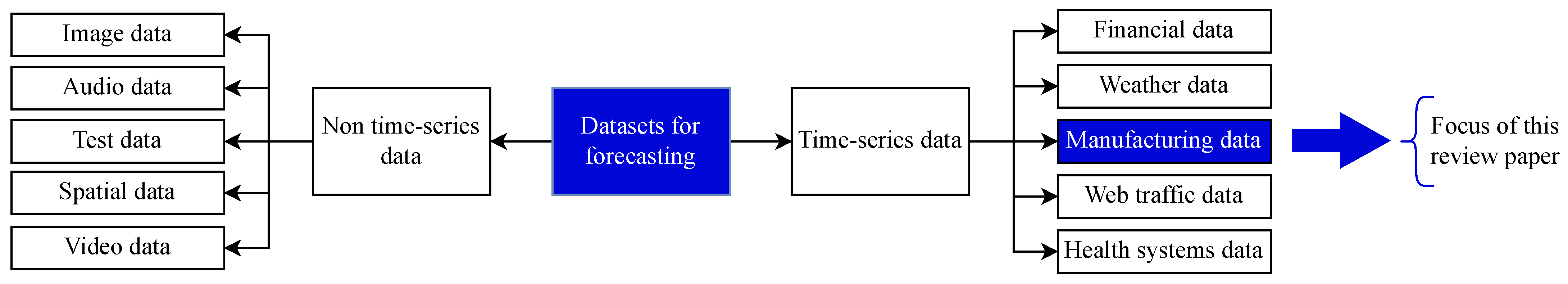
2. Time-Series Data

Time-series data are a set of observations recorded at consistent intervals. They have become a cornerstone in the analytical modeling of various domains due to their capacity to capture data trends and temporal features. Time-series forecasting, therefore, involves utilizing historical data points to predict future values, leveraging the inherent sequential band temporal nature of the data to unveil underlying patterns, seasonality, and trends. This predictive modeling technique is pivotal in numerous fields, such as finance, economics, and environmental science, where understanding and predicting future states is crucial for informed decision making.

A time-series sequence is a set of data points arranged chronologically, usually sampled at regular intervals. While this definition fits many applications, certain challenges can arise as follows:

• Missing data: It is common to encounter gaps in time-series data due to issues such as sensor malfunctions or data collection errors. Common strategies to address this include imputing the missing values or omitting the affected records [136].
• Outliers: Time-series data can sometimes contain anomalies or outliers. To handle these, one can either remove them using robust statistical methods or include them into the model [137].
• Irregular intervals: Data observed at inconsistent intervals are termed data streams when the volume is large or are simply termed unevenly spaced time-series. Models must account for this irregularity [132].

The right choice of model can directly address certain challenges. However, when data are gathered at inconsistent intervals, the model must be adjusted accordingly. While this review does not delve into time-series pre-processing, the research by Pruengkarn et al. [138] can be used as a resource for a thorough understanding of the matter.

Time-series data typically consist of three main components [139]:

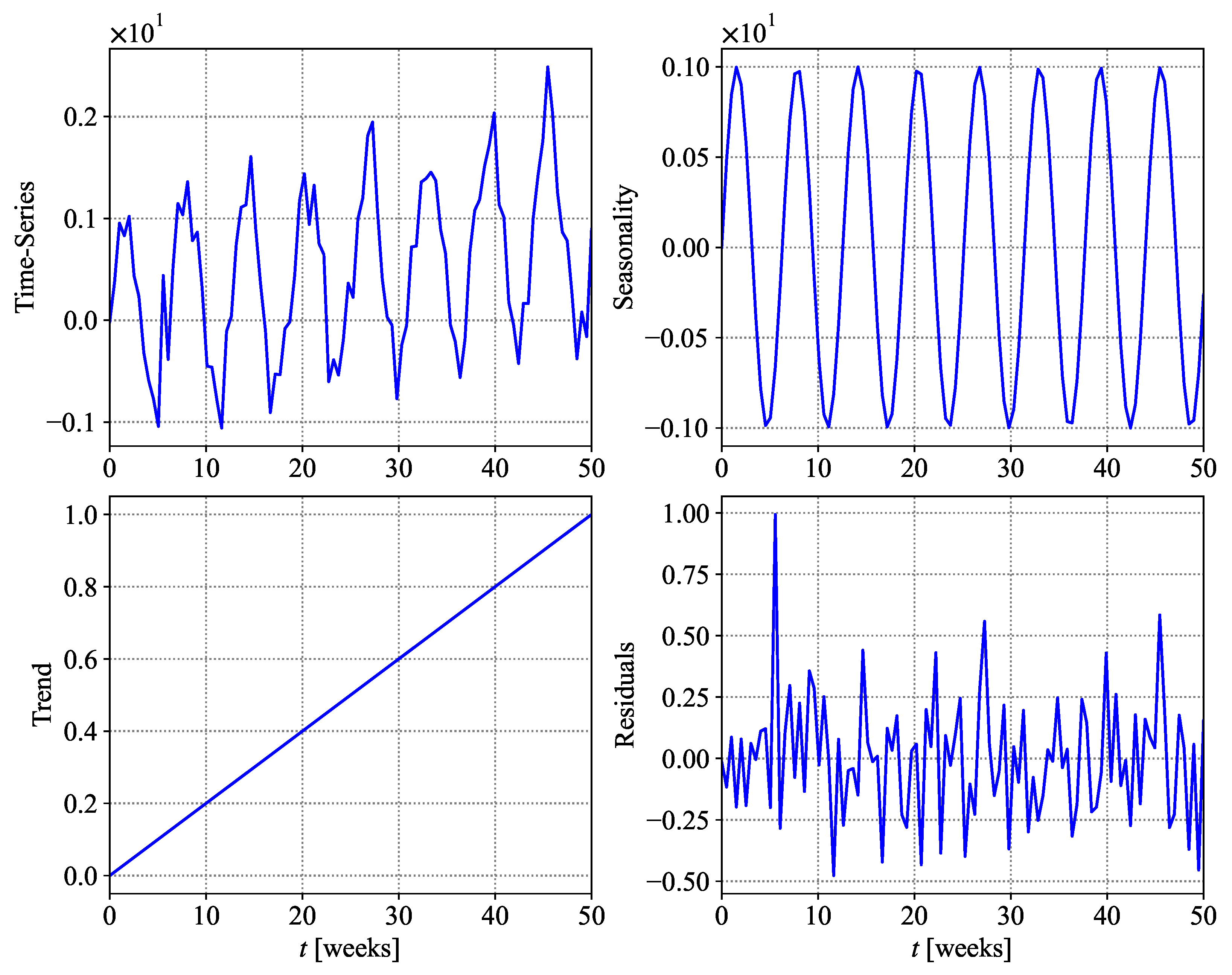
• Trend: This represents the direction in which the data move over time, excluding seasonal effects and irregularities. Trends can be linear, exponential, or parabolic.
• Seasonality: Patterns that recur at regular intervals fall under this component. Weather patterns, economic cycles, or holidays can induce seasonality.
• Residuals: After accounting for trend and seasonality, residuals remain. When these residuals are significant, they can overshadow the trend and seasonality. If the cause of these fluctuations can be identified, they can potentially signal upcoming changes in the trend.

In essence, a time-series is a combination of these components. An illustration of time-series data with seasonality, trends, and residuals is shown in Figure 5. Real-world data often have a significant irregular component, making them non-stationary (where mean and variance change over time). This irregularity makes forecasting challenging. Traditional forecasting methods often decompose a time-series into its components and predict each component separately. The success of a forecasting technique is often determined by its ability to predict the irregular component, where data mining techniques have proven especially effective.

2.1. Mathematical Representation

The time-series data can either be univariate (one time-dependent feature) or multivariate (more than one time-dependent feature). Time-series forecasting models are mostly designed to handle both types of input data. Hence, in this paper, no distinction has been made in model classification for both types of input data sets. However, below is a brief explanation for further understanding.

• Univariate time-series: Let $y=y(t-L),\dots ,y\left(t\right),y(t+1),\dots ,y(t+h)$ be a univariate time-series. It has L historical values, and $y(t-i)$ are the values of y for time $t-i$ where $i=0,\dots ,L$. The output of forecasting models is an estimated value of $y(t+1)$, often shown by $\widehat{y}(t+1)$. The objective function is to minimize the error $y(t+1)$ − $\widehat{y}(t+1)$.
• Multivariate time-series: The multivariate time-series can be represented in a matrix form as:

  $$\left[\begin{array}{c}{y}_1\\ y_2\\ ⋮\\ y_n\end{array}\right]=\left[\begin{array}{ccccc}{y}_1(t-L)& \dots & y_1\left(t\right)& \dots & y_1(t+h)\\ y_2(t-L)& \dots & y_2\left(t\right)& \dots & y_2(t+h)\\ ⋮& & ⋮& & ⋮\\ y_n(t-L)& \dots & y_n\left(t\right)& \dots & y_n(t+h)\end{array}\right]$$

  (1)

  where $y_i(t-m)$ is time-series data. Meanwhile, for historical data $i=\{1,2,\dots ,n\}$ and $m=\{0,1,\dots ,L\}$, $m=\{-1,-2,\dots ,-h\}$ represents the h future values.

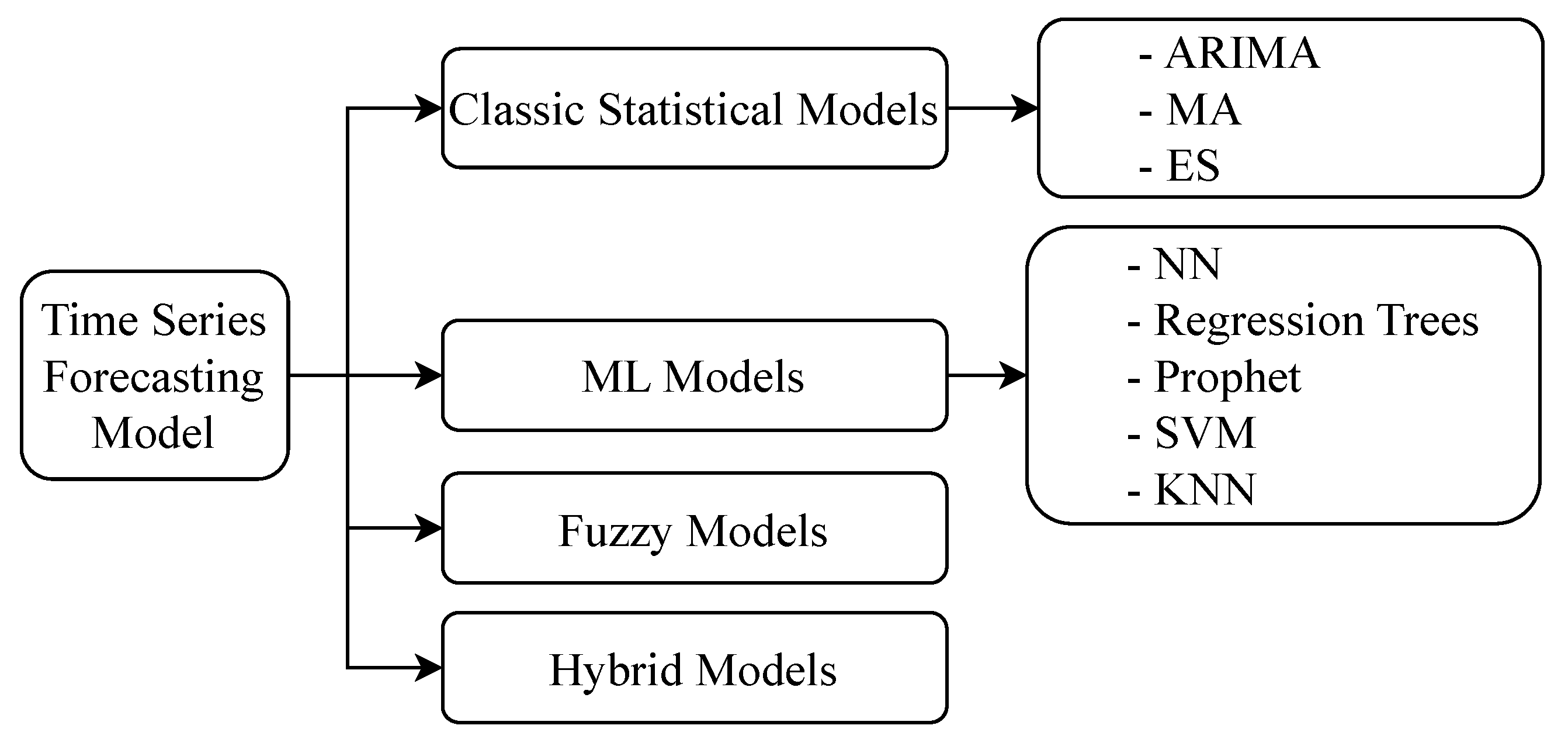
2.2. Time-Series Forecasting Models

Times-series forecasting is a critical and widely used technique in various fields, such as finance, economics, weather predictions, and energy management, among others [24,140,141,142]. It involves the development of statistical models to predict future values in a sequential dataset based on historical data [24,143].

Traditional statistical models include univariate methods, such as ARIMA [144], its seasonal variant Seasonal Autoregressive Integrated Moving Average (SARIMA) [24,143], and the Exponential Smoothing State-Space Model (ETS) [114]. Multivariate methods, like Vector Autoregression (VAR) [145] and Bayesian Structural Time-Series (BSTS) [146], consider multiple input variables, which can provide more accurate predictions in certain scenarios. ML models, such as SVM [54], regression trees [147], and Random Forests [68,148], have also been applied to time-series forecasting tasks. These models often require feature engineering to capture temporal features of data [149]. In recent years, Deep Learning-based models have emerged as a powerful tool for time-series forecasting. Long Short-Term Memory (LSTM) networks [105] and Gated Recurrent Unit (GRU) [150] are two widely used RNN architectures that can capture long-range dependencies in sequential data. Convolutional Neural Network (CNN) [151] and Transformer-based models, such as the Time-Series Transformer (TST) [112,152], have also been tested for time-series forecasting.

In this paper, we discuss nine of the time-series forecasting models, including ANN, ARIMA, MA and ES, regression trees, Prophet, k-Nearest Neighbors (KNN), SVM, Fuzzy models, and some hybrid models. Their wider categories are shown in Figure 6.

3. Time-Series Algorithms

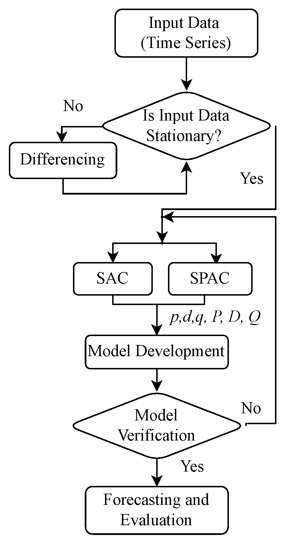
3.1. Autoregressive Integrated Moving Average

The ARIMA model is a well established and conventional technique for time-series forecasting, particularly for univariate data [24,35,144,153]. ARIMA models rely on a combination of three components: (i) AR, (ii) differencing (I), and (iii) MA to capture the underlying patterns and dependencies within a given time-series [143,154]. The AR function represents the dependence of a data point on its previous observations (lags), taking into account the time lag and coefficients. The MA component models the error terms by considering the dependency on previous error terms and their respective coefficients [26,155,156]. Finally, the I component refers to the differencing applied to the dataset to ensure stationarity by excluding trends and seasonality. Figure 7 presents an overall flow of ARIMA, including with Sample Autocorrelation (SAC) and Sample Partial Autocorrelation (SPAC). ARIMA models are represented by the notation ARIMA $(p,d,q)$, where p is the parameter for AR order, d is the degree of differencing for the I function, and q is the order of the MA component [143,144]. The appropriate values for p, d, and q are typically evaluated using Information Criterion (AICAkaike) or the Bayesian Information Criterion (BIC) for model selection [157,158,159,160].

In this model, the autoregression part uses the data from previous time steps to forecast future time steps using the regression function. The integrated part transforms non-stationary time-series input data to stationary data using differencing. This process is continued until stable data series are obtained. The moving average calculates the average in a fixed time window [161].

• AR component (order p): This component captures the dependency between an observation and several lagged observations.

  $$X_t=\beta +{\alpha }_1{X}_{t-1}+{\alpha }_2{X}_{t-2}+\cdots +{\alpha }_p{X}_{t-p}+{ϵ}_t$$

  (2)

  Here, $X_t$ is the lag of the time-series data, $\alpha$ is the coefficient of lag that is estimated by the model, $\beta$ is the intercept value or a constant, $ϵ$ is the error term, and p is the lag order.
• I component (order d): This component concerns differencing the time-series to make it stationary.

  $${\nabla }^d{X}_t=X_t-X_{t-1}$$

  (3)
• MA component (order q): This component applies a moving average model to lagged observations using the observation and its error term $ϵ$.

  $$X_t=\mu +{ϵ}_t+{\theta }_1{ϵ}_{t-1}+{\theta }_2{ϵ}_{t-2}+\cdots +{\theta }_q{e}_{t-q}$$

  (4)

  The $ϵ$ terms are from the AR models of lagged observations.

Combining the AR and MA, we obtain

$$\begin{array}{cc}\hfill X_t& =\beta +{\alpha }_1{X}_{t-1}+{\alpha }_2{X}_{t-2}+\cdots +{\alpha }_p{X}_{t-p}+{\theta }_1{ϵ}_{t-1}\hfill \\ \hfill & +{\theta }_2{ϵ}_{t-2}+\cdots +{\theta }_q{ϵ}_{t-q}\hfill \end{array}$$

(5)

Applications of ARIMA in Manufacturing Systems

In industrial applications, ARIMA models have been employed to forecast different data types, such as demand, production, and inventory levels, providing valuable insights for their respective sectors. In the power industry, Contreras et al. [26] used ARIMA models to predict the price for electricity load using the current day’s use, reporting an MAPE of 4.4% to 7.9% and demonstrating the model’s ability to produce accurate forecasts. Similarly, De Felice et al. [27] applied ARIMA models to predict short-term weather forecasts for demand forecasting in the energy sector, achieving a significant reduction in forecast error compared with persistence forecasts. In manufacturing, Torres et al. [28] employed ARIMA models to forecast the monthly production of laminated plastics in Spain, obtaining an MAPE of 4.96% and outperforming other techniques such as ES. Wang et al. [29] applied ARIMA to forecast monthly steel production in China, achieving an Mean Absolute Error (MAE) of 0.0797 and Root Mean Squared Error (RMSE) of 0.1055, highlighting the model’s effectiveness in capturing the underlying patterns in the data. In the oil and gas industry, Huang et al. [30] implemented ARIMA models for crude oil price forecasting, achieving an MAPE of 6.26% and demonstrating the model’s ability to outperform other techniques, including Generalized AutoRegressive Conditional Heteroskedasticity (GARCH) and ETS. Yu et al. [31] employed ARIMA to predict natural gas consumption in China, obtaining an MAPE of 4.17% and a Theil’s U statistic of 0.069, indicating the model’s superiority over the traditional least squares method. In the transportation sector, Williams et al. [32] used ARIMA models to forecast traffic volumes on highways, achieving a 6% improvement in forecast accuracy compared with the traditional MA model. Vlahogianni et al. [33] applied ARIMA to predict short-term traffic flow, reporting an MAPE of 8.9% and demonstrating the model’s potential for improving traffic management and infrastructure planning. Despite the success of ARIMA models in various industrial data forecasting applications, certain limitations, such as the assumption of linearity and the need for data to be stationary, persist [35,144]. To address these limitations and improve forecasting performance, researchers have explored hybrid models that combine ARIMA with other techniques, such as ML algorithms or ANNs [34,162].

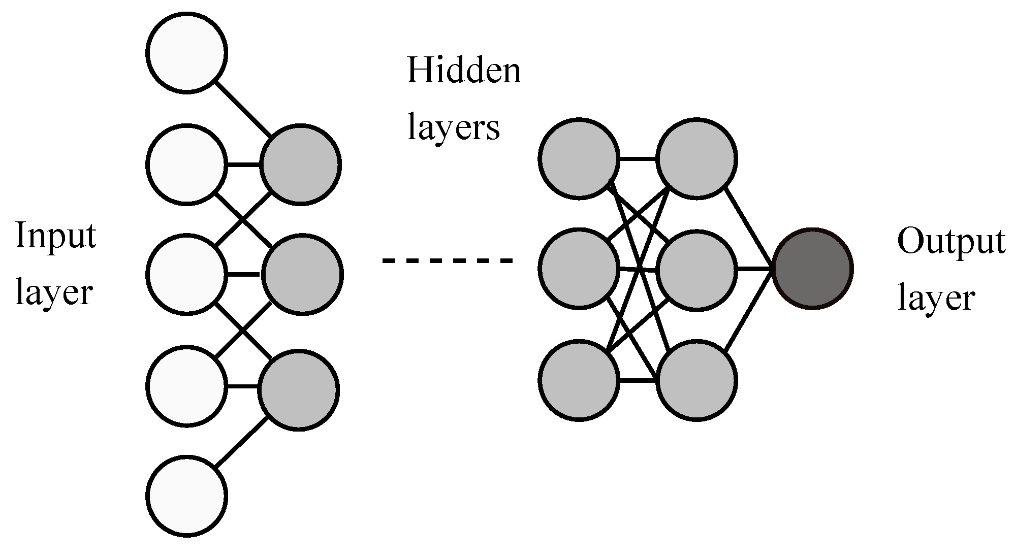
3.2. Artificial Neural Network

ANN are computational models inspired by the function of neurons and the network of neurons in the human brain. These networks are created from the interconnection of nodes or neurons that process information in three layers: (i) input, (ii) hidden, and (iii) output. Each connection between these nodes has an associated weight, which acts as a parameter and is tuned during the training process to minimize the difference between the predicted and actual outputs [163]. The ANNs have gained popularity in many disciplines, including time-series forecasting, due to their ability to model complex non-linear relationships without a priori assumptions about the data structure. They can capture intricate patterns, trends, and seasonality in time-series data, making them suitable for various forecasting tasks, from stock market predictions to energy consumption forecasts [90].

Training an ANN involves feeding it historical time-series data, allowing the network to learn the underlying patterns. Once trained, the ANN can predict future values. The backpropagation algorithm is commonly used for training, adjusting the weights in the network to minimize the prediction error [164]. In recent years, more advanced neural network architectures, such as LSTM networks and GRUs, have been introduced specifically to handle time-series data. These architectures can remember long-term dependencies in the data, making them particularly effective for forecasting tasks [105].

3.2.1. Feed-Forward Neural Networks

The FFNNs are among the simplest types of ANN. In an FFNN, the flow of information is unidirectional, and it only propagates in the forward direction, hence the name. The information flows from the input nodes, passing through the hidden layers and reaching the output nodes. There are no cycles or loops in the architecture [163]. The basic architecture of an FFNN is in Figure 8. The primary advantage of FFNNs is their ability to approximate any function given a sufficient number of hidden layers and nodes. This universal approximation capability makes them particularly suitable for modeling non-linear relationships, often observed in time-series data [165].

An FFNN can be mathematically represented by the composition of multiple functions, one for each layer [166]. For a simple FFNN with one hidden layer, the equations can be represented as:

$$\begin{array}{cc}\hfill h& =\sigma (W_{1}x+b_1)\hfill \end{array}$$

(6)

$$\begin{array}{cc}\hfill y& =\sigma (W_{2}h+b_2)\hfill \end{array}$$

(7)

where x is the input vector. $W_1$ and $W_2$ are weight matrices for the input and hidden layers, respectively. $b_1$ and $b_2$ are bias vectors for the input and hidden layers, respectively. $\sigma$ is the activation function, which is tuned according to the application and environment. The most used activation functions are logistic, sigmoid, Rectified Linear Unit (ReLU), and $tanh$. h is the output of the hidden layer, and y is the final output of the network. In time-series forecasting, FFNNs can be trained to predict trends in the data using historical values. The input layer typically consists of nodes representing previous time steps, while the output layer represents future time steps. The hidden layers capture the underlying patterns and relationships in the data. Training involves adjusting the network weights to minimize the difference between the ground truth and actual values [140]. However, while FFNNs can be powerful, they also come with challenges. They can easily overfit the training data if they are not adequately regularized, and their “black box” nature can make them difficult to interpret. Despite these challenges, FFNNs have been successfully applied in various time-series forecasting tasks, from stock market prediction to energy consumption forecasting [167].

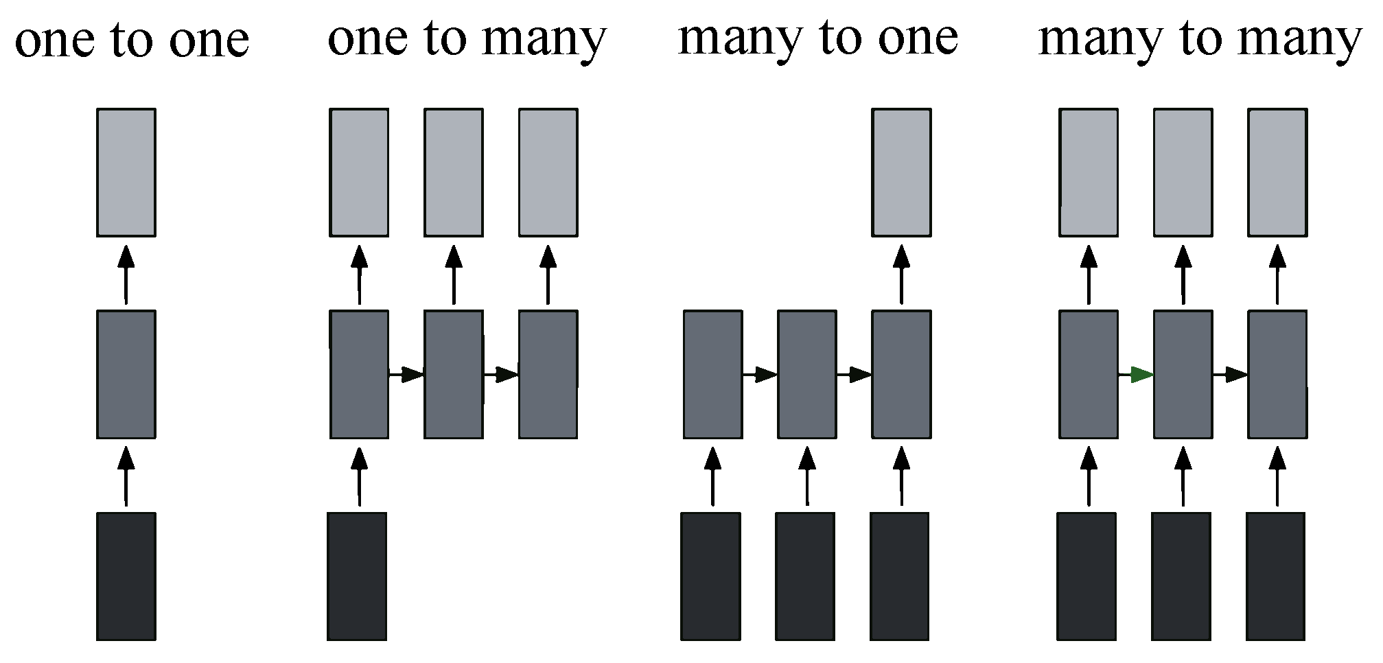
3.2.2. Recurrent Neural Networks

RNNs are a subset of neural networks designed to identify patterns in data, such as time-series, image, audio, or text data. Unlike traditional feed-forward neural networks, RNNs have connections that loop back on themselves, which allows the information to be retained [168]. Various architectures of RNNs are shown in Figure 9. These various architectures include:

• Singular input–Singular output configuration (one-to-one): This configuration represents the classic feed-forward neural network structure, characterized by a solitary input and the expectation of a single output.
• Singular input–Multiple output configuration (one-to-many): In the context of image captioning, this configuration is aptly illustrated. A single image serves as a fixed-size input, while the output comprises words or sentences of varying lengths, making it adaptable to diverse textual descriptions.
• Multiple input–Singular output configuration (many-to-one): This configuration finds its application in sentiment classification tasks. Here, the input is anticipated to be a sequence of words or even paragraphs, while the output takes the form of continuous values, reflecting the likelihood of a positive sentiment.
• Multiple input–Multiple output configuration (many-to-many): This versatile model suits tasks such as machine translation, reminiscent of services like Google Translate. It is well suited to handle inputs of varying lengths, such as English sentences, and producing corresponding sentences in different languages. Additionally, it is applicable to video classification at the frame level, requiring the neural network to process each frame individually. Due to interdependencies among frames, recurrent neural networks become essential for propagating hidden states from one frame to the next in this particular configuration.

Mathematically, the hidden state $h_t$ of a simple RNN at time t is given by:

$$h_t=\sigma (W_{hh}{h}_{t-1}+W_{xh}{x}_t+b_h)$$

(8)

where $x_t$ represents the input at instance t. $h_{t-1}$ denotes the hidden state at the instance $(t-1)$. $W_{hh}$ and $W_{xh}$ are the weight matrices. $b_h$ is the bias term and can be a constant. $\sigma$ is the activation function. The output $y_t$ at time t is then expressed as:

$$y_t=W_{hy}{h}_t+b_y$$

(9)

RNNs are especially suitable for forecasting as they are designed to remember previous inputs in their hidden state, which enables them to capture temporal dependencies [169]. However, traditional RNNs can face challenges with long-term dependencies because of issues such as vanishing and exploding gradients. To address these challenges, variants such as LSTM and GRU networks have been introduced [105].

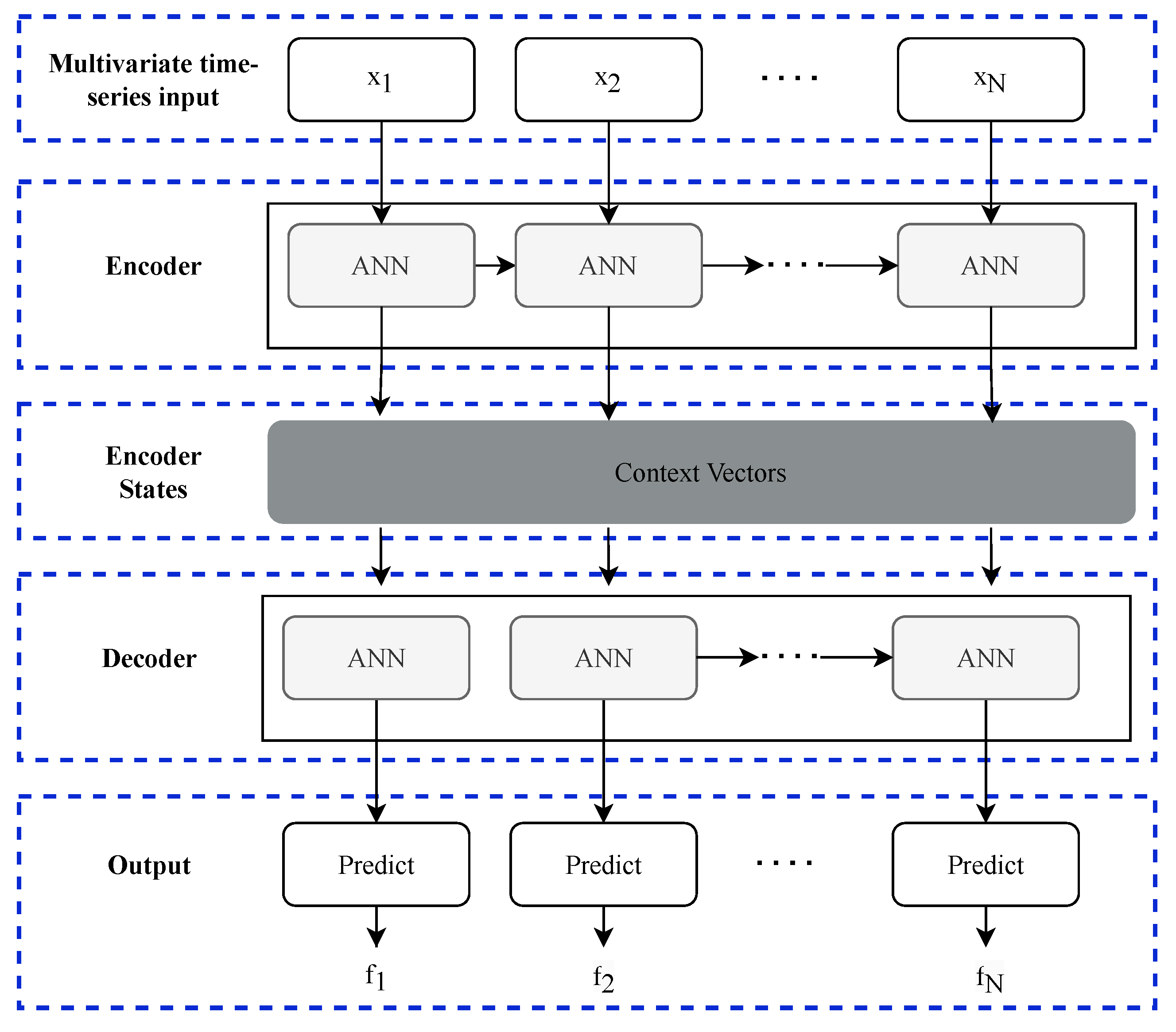
3.2.3. Encoder-Decoder Architecture

The input to the ANN can contain multivariate features related to the manufacturing process, such as equipment temperatures and vibrations, production counts, and energy consumption. The output is a forecast of future values for these variables, allowing us to anticipate potential issues and optimize operations accordingly. In most cases, the neural network takes in a sequence of past observations and predicts the next single time step. This approach is straightforward and suitable for applications with sufficient short-term predictions. Standalone models such as LSTM or GRU can be used in these scenarios. However, predicting a sequence of future time steps is often necessary for long-term forecasting. This is typically achieved using an encoder-decoder architecture [170]. The overall structure of the encoder-decoder-based architecture is shown in Figure 10.

Encoder: The encoder processes the input sequence and compresses the information into a fixed-size context vector. This is also called a latent vector. The encoder is typically implemented using an RNN, LSTM, or GRU. The final hidden state from the last time step of the network serves as the context vector [171,172].

Decoder: The decoder takes the context vector provided by the encoder and generates the output sequence, which can be a forecast of future values. The decoder also typically uses LSTM cells. The decoder generates the output sequence one step at a time. For multi-step forecasting, the decoder can be used recursively, where the predicted output at each time step is fed back as an input to predict the next time step.

The encoder-decoder architecture effectively captures long-range temporal dependencies in time-series data and can handle variable-length output sequences, making it suitable for multi-step forecasting. The recursive application of the decoder is useful for long-term predictions.

3.2.4. Applications of ANNs in Manufacturing Systems

The RNNs, especially their advanced variants such as LSTM networks, have gained importance as time-series forecasting models due to their ability to capture temporal dependencies [105]. In manufacturing systems, the application of RNNs has been particularly promising. One of the primary applications in manufacturing is demand forecasting. Accurate demand forecasts enable manufacturers to optimize inventory, reduce costs, and improve service levels. Zhao et al. [107] employed LSTM networks to predict product demand and found that they outperformed traditional methods, especially when the demand patterns were non-linear and had long-term dependencies.

Predictive maintenance is another crucial application in manufacturing. Manufacturers can reduce downtime and increase operational efficiency by predicting machine failures before they occur. Malhotra et al. [95] demonstrated that RNNs could effectively predict the remaining useful life of machines, leading to more timely maintenance. Furthermore, quality control is paramount in manufacturing. Li et al. [96] utilized RNNs to forecast the quality of products in real time, allowing for immediate corrective actions and ensuring consistent product quality.

The LSTM networks have become popular as time-series forecasting models due to their ability to capture long-term dependencies and model sequential data effectively [105]. Accurate demand prediction is crucial for efficient inventory management and production planning. Studies have shown that LSTMs, when trained on historical sales data, can outperform traditional time-series forecasting methods in predicting future product demand [84]. LSTMs have been employed in quality control, where they assist in predicting the quality of products based on various parameters and sensor readings during the manufacturing process. This predictive quality control approach helps in the early detection of defects and reduces waste [3]. The biggest challenge for LSTMs is their black box nature, making them difficult to interpret, which can be a concern in critical manufacturing processes. Moreover, training LSTMs requires significant computational resources, especially for large datasets [84].

Recently, the use of encoder-decoder-based architectures, employing variations of LSTMs and GRUs, has become popular due to its ability to capture long-term data trends. One such framework has been presented to predict multiple future time steps simultaneously for energy load forecasting. For point forecast, the Transformers-based model performed the best with an RMSE of 29.7% for electricity consumption and an RMSE of 8.7% for heating load. Meanwhile, recurrent models such as LSTMs and GRUs have shown good results for quantile forecasts [173]. Another study presented a predictive maintenance model for NOx sensors in trucks using an encoder-decoder LSTM network combined with a Multiple Linear Regression model to forecast sensor failures. The results show improved performance when compared with the baseline models, and the authors presented a generalized approach for other sensor applications [174]. An attention-based RNN encoder-decoder framework was used for multi-step predictions using historical multivariate sensory time-series data, leveraging spatial, parameter-wise, and temporal correlations. For air quality monitoring data, this model outperforms existing baseline models in prediction accuracy [175]. Another paper proposes an attentive encoder-decoder model with non-linear multilayer correctors for short-term electricity consumption forecasting [176]. Another study introduced an asymmetric encoder-decoder framework using CNN and a regression-based NN to capture spatial and temporal dependencies in energy consumption data from 10 university buildings in China. The results showed an average $R^2$ of 0.964, and for multi-step forecasting, the results showed an average $R^2$ of 0.915 for three steps ahead [177]. Another interesting framework was presented, which used a double encoder-decoder model to improve electricity consumption prediction accuracy in manufacturing. Using two separate encoders for long-term and short-term data, the model outperformed traditional methods, reducing mean absolute error by about 10% when tested on data from a manufacturing site [178]. Another study developed a sequence-to-sequence GRU model to predict future reheater metal temperatures in coal power stations during flexible operations. The model achieved an MAPE below 1%, indicating high accuracy [179].

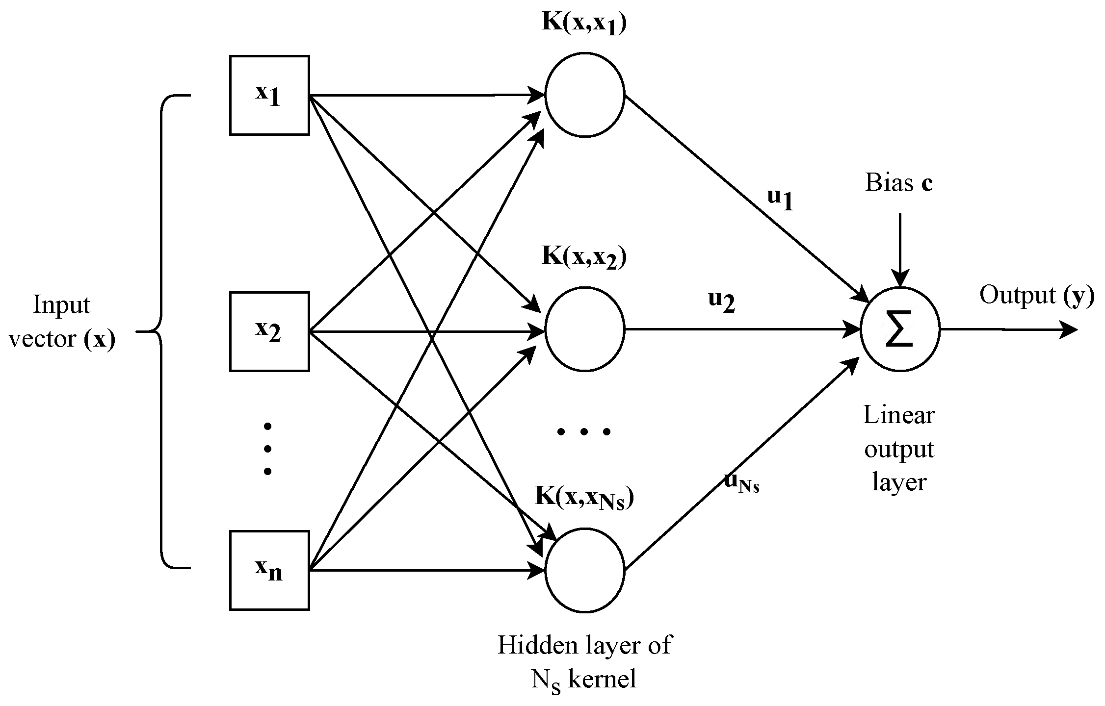
3.3. Support Vector Machines Models

SVMs, (as shown in Figure 11), have become a powerful tool for industrial time-series forecasting, offering promising results in various applications [180]. SVMs have shown promising results in forecasting different types of time-series data, such as finance, energy, manufacturing, and transportation [57]. It works as a supervised learning model primarily designed for classification and regression targets. Introduced by Vapnik [180], SVMs predict a continuous value or a class by finding the optimal hyperplane that best separates data. In time-series forecasting, SVMs are used as regression tools, often referred to as Support Vector Regression (SVR). SVR has f as the objective function that computes the deviation $ϵ$ from the actual training responses while also being as flat as possible [55].

Given a training set $\{(x_1,y_1),\dots ,(x_n,y_n)\}$, SVR aims to find its objective function f such that:

$$y_i-f\left(x_i\right)\le ϵ$$

(10)

where $x_i$ is the input and $y_i$ is the output and with the optimal weight vector as:

$$w=\sum _{i=1}^n\left({\alpha }_i{y}_i\right)\varphi \left(x_i\right)$$

(11)

where ${\alpha }_i$ represents the Lagrange multiplier coefficients. The function f is represented as:

$$f\left(x\right)=\sum _{i=1}^n{u}_{i}K(x,x_i)+c$$

(12)

where $u_i={\alpha }_i{y}_i$, $K(x,x_i)=\varphi {\left(x_i\right)}^T\varphi \left(x\right)$ is a kernel function, such as the polynomial or linear kernel, and c is a bias term that can be a constant [181].

SVMs, with their ability to handle non-linear relationships through the kernel trick, are able to capture intricate patterns in the data.

Applications of SVMs in Manufacturing Systems

One significant advantage of SVMs is their ability to handle non-linear and complex features in the training data [54]. Traditional linear models, such as ARIMA, may fail to capture such patterns, leading to suboptimal predictions. In contrast, SVMs use kernel functions, which map the input data into a higher dimensional space, which provides a more flexible and accurate representation of non-linear relationships [181] between input and output metrics. Another key advantage of SVMs is their robustness to overfitting [55]. The SVM algorithm seeks to maximize the margin between classes, resulting in a thinly distributed solution that relies only on a subset of the training data (i.e., support vectors). This approach reduces the model’s complexity, making it less prone to overfitting and improving its generalization performance. Several studies have demonstrated the effectiveness of SVMs in industrial time-series forecasting. For instance, Tay and Cao [56] compared the forecasting performance of SVMs and other methods, such as ARIMA and backpropagation neural networks, on the Taiwan Stock Exchange Weighted Index. Their results showed that SVMs outperformed the other methods based on MAPE. Similarly, Cao and Tay [54] applied SVMs to predict the Singapore Stock Market Index and found that SVMs achieved better forecasting accuracy than both ARIMA and FFNN. In the energy sector, Huan et al. [57] used SVMs to forecast monthly electricity consumption in China. Their study revealed that SVMs provided more accurate forecasts than classic statistical models, such as ARIMA and ES. In another study, Guo et al. [58] employed SVMs for short-term wind power forecasting and showed that SVMs outperformed several Machine Learning algorithms, including ANN and decision trees.

3.4. Fuzzy Network Models

Fuzzy Neural Networks (FNNs) employ the learning capability of neural networks along with the reasoning of Fuzzy Logic Systems [100]. Fuzzy Neural Networks are particularly useful for modeling complex systems where the relationships between variables are not clear or are non-linear [101]. Mathematically, an FNN for time-series forecasting can be represented as a combination of fuzzy rules and neural network structures. Consider a simple Fuzzy Neural Network (FNN) with one input $x_t$:

$$y_t=\sum _{i=1}^n{w}_i\times f_i\left(x_t\right)$$

(13)

where $y_t$ is the forecasted value and $x_t$ is the observed value at instance t. $w_i$s are the weights associated with each fuzzy rule. $f_i$s are the fuzzy membership functions. n is the number of fuzzy rules.

The weights $w_i$ are typically learned using a learning algorithm, such as backpropagation, while the membership functions $f_i$ are determined using fuzzy clustering techniques or expert knowledge [182]. FNNs have been successfully applied to various time-series forecasting tasks, offering the advantage of capturing the inherent uncertainty and vagueness in the data, often present in real-world time-series [90].

Applications of Fuzzy Networks in Manufacturing Systems

FNNs have been applied to industrial time-series forecasting and have demonstrated superior performance compared with traditional forecasting methods. For instance, Yager and Filev [183] proposed a fuzzy neural network model for forecasting electricity consumption and achieved better accuracy compared with other traditional models. Another approach is the Adaptive Neuro-Fuzzy Inference System (ANFIS), which combines the fuzzy logic system with the adaptive learning capabilities of neural networks [101]. ANFIS has been successfully applied to various time-series forecasting tasks in industrial settings. For example, Aladag et al. [102] employed ANFIS for time-series forecasting in the textile industry, resulting in improved prediction accuracy compared with traditional time-series models. Fuzzy rule-based systems have also been utilized for industrial time-series forecasting. Fuzzy Time-Series (FTS) models, introduced by [103], represent the time-series data using fuzzy sets and linguistic variables, allowing for better handling of uncertainties and vagueness. Lee and Hong [104] applied FTS to industrial production index forecasting, showing its effectiveness in comparison with other traditional forecasting techniques.

3.5. Prophet

Prophet, developed by Meta, the parent company of Facebook, is a model specially designed for forecasting time-series data with prominent seasonal effects and historical data. It demonstrates resilience when dealing with missing data and changes in the trend, and it generally performs effectively when handling outlier values [81]. The core of the Prophet model has three main components: (i) trend, (ii) seasonality, and (iii) holidays. Mathematically, Prophet can be represented as:

$$y\left(t\right)=g\left(t\right)+s\left(t\right)+h\left(t\right)+{ϵ}_t$$

(14)

where $y\left(t\right)$ is the forecast value of the target metric; $g\left(t\right)$ represents the trend function, which models changes in inconsistent intervals. $s\left(t\right)$ captures periodic changes, i.e., seasonality. $h\left(t\right)$ is the function for holidays, and ${ϵ}_t$ accounts for the error, which is usually a normally distributed function.

The trend function $g\left(t\right)$ is typically modeled using a piece-wise linear or logistic growth curve. Seasonal effects $s\left(t\right)$ are modeled using the Fourier series. Holidays and events $h\left(t\right)$ provide a flexible way to model special events that do not fit into the regular seasonality [81]. Prophet’s flexibility and ease of use have made it a popular choice for time-series forecasting in various applications, from business forecasting to academic research. The application of Prophet in time-series forecasting for manufacturing systems is promising, offering a blend of adaptability and accuracy. As more manufacturing entities adopt and adapt this tool, its methodologies will likely evolve, leading to even more refined forecasting models tailored to the unique challenges of the manufacturing sector.

3.6. k-Nearest Neighbors Models

The KNN models offer a simple yet effective approach for predicting future values based on historical data for time-series datasets. The KNN algorithm relies on the similarity between instances, using the k most similar instances (neighbors) in the training set to make predictions for new instances. Different methods are used to measure similarity in time-series data. The Euclidean distance is the most common method, which measures the straight-line distance between two points in multidimensional space. It is rather simple and computationally efficient but can become sensitive to amplitude differences and time shifts. Dynamic Time Warping is used to align time-series that vary in speed and time shifts. This effectively handles time deformations but is computationally intensive. Correlation-based measures are used to evaluate the correlation between time-series values. The main disadvantage is that it can capture linear relationships but may miss non-linear dependencies. Cosine similarity is also popular as it measures the cosine of the angle between two vectors. Focusing on directional similarity makes it less sensitive to magnitude differences [184].

In the energy sector, Mahaset et al. [185] utilized a KNN-based approach for short-term wind speed forecasting, demonstrating improved prediction accuracy compared with traditional time-series models. This accurate wind speed forecasting is essential for efficiently integrating wind energy into power grids. In finance, Arroyo et al. [186] applied KNN models to predict stock prices and achieved satisfactory performance compared with other Machine Learning techniques. Their study highlights the potential of KNN models in assisting investors and financial analysts in making informed decisions. In transportation, Vlahogianni et al. [33] presented a KNN-based approach for traffic flow prediction in urban networks, showing better performance than traditional time-series models. The accurate prediction of traffic flow can help in the development of effective traffic management strategies and reduce congestion. In the manufacturing sector, Al-Garadi et al. [187] applied KNN models to predict equipment failure in industrial machines, demonstrating the effectiveness of the KNN algorithm in detecting machine anomalies and improving maintenance scheduling.

3.7. Generative Adversarial Network

The GAN is a DL model composed of two neural networks competing against each other. One is called the generator, and the other is the discriminator. The generator attempts to produce synthetic data samples, while the discriminator evaluates the difference between the generated and real data samples. The aim is to improve the generator’s ability to create indistinguishable data from real data. GANs have been explored for time-series forecasting in recent years with promising results. They can capture complex and high-dimensional patterns in the data, making them particularly useful in cases where traditional statistical methods fail. They can have various applications in forecasting systems, from generating new features to direct predictions. These are explained as follows:

• Generating synthetic time-series data: The generator of a GAN can learn the underlying data distribution of a time-series dataset and generate new data that mimics the real data. This can be particularly useful when there is a lack of data or when data augmentation is needed [188].
• Anomaly detection: GANs can be trained to reconstruct normal time-series data. It can be considered an anomaly if the network fails to reconstruct a data point properly. This is particularly useful in cybersecurity or preventive maintenance [189].
• Direct predictions: GANs have also been directly used for time-series forecasting by training the generator to predict future data points based on previous ones. The discriminator is then trained to evaluate the difference between true and predicted future values. The generator tries to trick the discriminator into believing that the predictions are real future values [190].

3.8. Hybrid Models

Hybrid models have emerged as an effective approach for industrial time-series forecasting by combining the strengths of different fundamental methods to achieve better prediction performance. These models have been applied across various industries, such as energy, finance, manufacturing, and transportation, demonstrating promising results and improved forecasting accuracy. Empirical Mode Decomposition (EMD) uses the multi-resolution method to separate the input signal into multiple meaningful components. It can be used to forecast non-linear and non-stationary datasets by decomposing them into components of different resolutions. In the energy sector, Mandal et al. [191] developed a hybrid model combining wavelet transform and ANN to forecast short-term loads in power systems. Their approach significantly improved the forecasting accuracy compared with individual methods, highlighting the effectiveness of hybrid models in capturing complex patterns in time-series data. In finance, Zhang and Qi [192] proposed a hybrid model that integrated a Genetic Algorithm (GA) and SVM for stock market forecasting. Their approach outperformed traditional time-series models and individual ML techniques, emphasizing the potential of hybrid models for financial time-series forecasting tasks. In transportation, Kamarianakis et al. [193] employed a model that combined the ARIMA model with a KNN model for short-term traffic flow prediction. Their model demonstrated superior performance compared with individual methods, offering a more accurate and robust forecasting approach for traffic management. In manufacturing, Baruah and Chinnman [194] developed a hybrid model that combined Principal Component Analysis with neural networks for forecasting tool wear in machining operations. Their approach achieved better prediction accuracy than traditional time-series models, suggesting that hybrid models can effectively support predictive maintenance and quality control in manufacturing processes.

CNNs, when combined with other models, are also useful for forecasting. Wahid et al. proposed a hybrid CNN-LSTM framework for predictive maintenance in Industry 4.0, combining CNN to extract features and LSTM to capture long-term dependencies of data. The model effectively predicted machine failures using time-series data [195]. In another paper, CNN combined with LSTM was used to predict the production progress of manufacturing workshops using transfer learning. The results show an improved efficiency and accuracy compared with the baseline models [196]. Canizo et al. proposed a CNN–RNN architecture for supervised anomaly detection, eliminating the need for data pre-processing for multisensor time-series data. Using a separate CNN for each sensor, the model effectively addressed anomalies in an industrial service elevator [197]. DCGNet is a framework proposed by Zhang et al., which is a combination of CNN and GRU examined for forecasting sintering temperature in coal-fired equipment using multivariate time-series data. The results show high accuracy and robustness in predicting sintering temperature, which is critical for process control in industries like cement, aluminum, electricity, steel, and chemicals [198].

Hybrid models have demonstrated their potential in various industrial time-series forecasting tasks, offering improved performance and adaptability by combining the strengths of different methods. The continued development and application of hybrid models can potentially lead to more accurate and efficient predictions across various industries.

Table 2. Comparison of hybrid models for time-series forecasting in manufacturing systems.

Hybrid Models	Novelty
ARIMA + ANN	The ARIMA model is used to capture the periodic and linear elements in the training data, and the ANN is used to capture the non-linear features. This type of model can capture the linear and non-linear features in the training data, which has proven to be more useful for complex datasets.
Dynamic model + Fuzzy	The dynamic model can capture the temporal features in the datasets, and when it incorporates AR components, it can capture the linear dependencies in the data. The Fuzzy model captures the uncertainty in the dataset. This type of model is robust to the changing patterns in the underlying data.
ANN + Evolutionary	Multiple structures of ANN such as LSTM and RNN can be used to capture the complex patterns and dependencies in the data. The evolutionary algorithm part is used to optimize the hyperparameters of the underlying ANN model. This model can enhance the forecasting accuracy of the ANN and reduces overfitting.
ARIMA + SVM	ARIMA is effective at capturing the linear features in the data along with seasonality patterns. SVM captures the non-linear features in the residuals that are missed by ARIMA.
Ensemble + hybrid ANNs	The Ensemble ANN model combines the forecasts from multiple ANN models, which results in better accuracy. It is particularly useful for capturing the non-linear features in the training data.
Kernel-based SVRs	The kernel function allows SVR to perform non-linear regression and reduces the risk of over-fitting by using the subsets of training data as support vectors. Also, Vapnik’s Structural Risk Minimization Principle of SVR reduces the overall error by minimizing the upper bound on the generalization error.
EMD + AR + SVR	Hybridization of SVR with AR and different EMD methods.
Fuzzy Neuro	Fuzzy logic incorporates the uncertainty in the data, while the neural network is able to capture the non-linear relationships in the data. It is particularly useful when the dataset is complex and an understanding of the underlying processes is as important as the accuracy of the forecasts.
Fuzzy + SVM + Evolutionary	Fuzzy logic is used for handling data uncertainty, and the pattern recognition ability of SVM is used for accurate forecasting. The evolutionary algorithm provides the global optimization to fine tune the system. It is very useful in cases where the data can be highly volatile and ambiguous.

summarizes the novelties in various combinations of hybrid models in the existing literature related to applications in manufacturing and industrial automation.

4. Discussion of Time-Series Forecasting Models for Industrial Systems

Understanding the strengths and weaknesses of various time-series models is crucial for selecting the suitable forecasting method in an industrial setting. This paper comprehensively compares different time-series models applied to industrial forecasting tasks, including classic statistical models, ML techniques, and hybrid models. Traditional statistical models, such as ARIMA and ETS, have been widely used for industrial time-series forecasting due to their simplicity and interpretability [143]. These models have shown satisfactory performance in some cases, but they do not perform well when the dataset is more complex and has non-linear features [144,199]. Machine Learning techniques, such as SVM, KNN, and ANN, have emerged as promising alternatives to traditional models, offering better performance in capturing complex relationships and non-linearity in time-series data [185,200,201]. However, these models may require more computational resources and can be less interpretable than traditional models [33,54]. Deep Learning models, such as LSTM networks and CNN, have demonstrated superior performance in various industrial forecasting tasks by leveraging their ability to model long-term dependencies and handle high-dimensional data [105,166]. Despite their success, these models can be computationally expensive and may require large training data to achieve optimal performance. Hybrid models, which combine different techniques to leverage their strengths, have been proposed to overcome individual models’ limitations [193]. By integrating traditional models with Machine Learning or Deep Learning techniques, hybrid models have shown improved performance and adaptability in various industrial forecasting tasks. While GANs show potential in time-series forecasting, they also present challenges such as training difficulty and mode collapse. The use of GANs for time-series forecasting is an active area of research, and new techniques and refinements are being developed to address these challenges.

Table 3. Advantages and disadvantages of various forecasting models.

Model	Advantages	Disadvantages
ARIMA	- Handles linear relationships - Can model stationary time-series data	- Requires data to be stationary - Struggles with non-linear patterns
ANN	- Can model complex non-linear relationships - Flexible architecture	- Requires large datasets - Black box nature
RNN	- Can capture sequences and patterns over time - Suitable for time-series data	- Can struggle with long-term dependencies
LSTM	- Addresses vanishing gradient problem of RNNs - Can model long-term dependencies	- Computationally intensive - Requires careful tuning
KNN	- Non-parametric - Simple to understand	- Computationally expensive - Sensitive to irrelevant features
Fuzzy Networks	- Can handle uncertainty and vagueness - Flexible modeling	- Requires expert knowledge - Can be computationally intensive
Regression Models	- Interpretable - Can handle multiple predictors	- Assumes linear relationship - Sensitive to outliers
Prophet	- Handles seasonality and holidays - Robust to missing data	- Assumes additive model - Might require domain-specific adjustments
MeanAbsolute	- Simple to compute - Provides a baseline measure	- Does not capture complex patterns

provides an overview of the advantages and disadvantages of various models discussed in this review to provide a holistic reference for other researchers to identify a potentially suitable method for their applications.

5. Challenges and Research Directions

This section discusses the challenges and future directions pertaining to the use of data and data-driven approaches in time-series forecasting algorithms for industrial manufacturing systems.

5.1. Challenges

The rapid advancements in computational capabilities, data availability, and artificial intelligence can potentially revolutionize the future landscape of time-series forecasting models in the industrial environment. As industries become increasingly data-driven, the demand for accurate and reliable forecasting models will continue to grow, leading to new developments and innovations in time-series forecasting techniques. However, several challenges need to be addressed to fully realize these advancements:

• Data quality and pre-processing:

  −

  Inconsistent data: industrial data often come from various sources with different formats and frequencies, requiring significant pre-processing to ensure consistency.

  −

  Missing data: handling gaps in data and ensuring accurate imputation methods can be complex but is crucial for reliable forecasting.

  −

  Noise and outliers: industrial data can be noisy and can contain outliers that can distort model predictions, necessitating robust cleaning techniques.

• Computational complexity:

  −

  Scalability: advanced forecasting models, especially those involving Deep Learning, can be computationally intensive and may not scale efficiently with large datasets common in industrial settings.

  −

  Resource requirements: high computational power and memory requirements can be a barrier for many companies, particularly for small- and medium-sized enterprises.

• Model interpretability:

  −

  Black box nature: many advanced models, such as ANNs and other Deep Learning techniques, are often criticized for their lack of transparency, making it difficult for practitioners to trust and adopt them.

  −

  Explainability tools: developing and integrating tools that can provide insights into model decisions is essential to increase user trust and model acceptance.

• Integration with existing systems:

  −

  Compatibility issues: integrating new forecasting models with legacy systems and existing infrastructure can be challenging and requires careful planning and execution.

  −

  Maintenance and updates: ensuring that the models remain up to date with the latest data and perform well over time involves ongoing maintenance efforts.

• Real-time processing:

  −

  Latency: for many industrial applications, real-time or near-real-time forecasting is essential, requiring models and systems that can process data and generate predictions with minimal delay.

  −

  Streaming data: handling continuous data streams and updating models dynamically can be technically challenging but is crucial for timely decision making.

5.2. Future Directions

Here, we discuss several potential future directions for time-series forecasting models in industrial settings:

• Advanced Deep Learning models: The development and application of advanced Deep Learning models, such as transformers and attention mechanisms, can potentially improve the performance of time-series forecasting in industrial systems by capturing complex, high-dimensional, and long-term dependencies in data.
• Ensemble and hybrid approaches: Combining multiple forecasting models, including ensemble techniques and hybrid approaches, can lead to more robust and accurate predictions by leveraging the strengths of different methods and mitigating individual model weaknesses.
• Transfer Learning and Meta-Learning: Applying Transfer Learning and Meta-Learning techniques can potentially improve the generalization of time-series forecasting models across different industries and tasks, enabling the reuse of knowledge learned from one domain to another, thus reducing the need for extensive domain-specific training data.
• Explainable AI: The need for explainable and interpretable models will grow as industries increasingly adopt AI-based forecasting models; developing explainable time-series forecasting models can help decision makers understand the patterns and underlying features in data, leading to more informed decisions and better model trust.
• Real-time and adaptive forecasting: With the increasing availability of real-time data in industrial systems, developing time-series forecasting models that can adapt to changing patterns and trends in real-time will become increasingly important; these models can enable industries to respond quickly to unforeseen events and dynamically optimize operations.
• Integration with other data sources: Incorporating auxiliary information, such as external factors and contextual data, can potentially improve the performance of time-series forecasting models; future research may focus on integrating multiple data sources and modalities to enhance prediction accuracy in industrial settings.
• Domain-specific models: As time-series forecasting techniques evolve, future research may focus on developing domain-specific models tailored to specific industries’ unique requirements and challenges, such as energy, finance, manufacturing, and transportation.

6. Conclusions

In conclusion, time-series forecasting models are critical in various industrial systems, enabling more efficient decision making, resource allocation, and overall operational optimization. Numerous forecasting models have been applied across the energy, finance, manufacturing, and transportation industries, including traditional statistical methods, ML techniques, and hybrid approaches. Traditional statistical methods, such as ARIMA and ES, provide a solid foundation for time-series forecasting and are widely used due to their simplicity and interpretability. However, these models may struggle with complex, non-linear, and high-dimensional data, common in industrial systems. Machine Learning techniques, including KNN, SVM, Fuzzy Network Models, and ANN, offer more flexibility and adaptability for handling complex data patterns in industrial time-series forecasting tasks. These models have shown promising results in various industries, often outperforming traditional statistical methods. Hybrid models have emerged as an effective approach to improve forecasting performance, further using the best features from different modeling techniques. These models can leverage the advantages of various techniques to achieve better prediction accuracy and robustness in industrial time-series forecasting tasks. Each model has its strengths and weaknesses, and choosing the most suitable model depends on the specific industry, data characteristics, and forecasting objectives. It is essential for practitioners and researchers to carefully evaluate the performance in terms of the flexibility, robustness, and forecasting accuracy of different models and adopt a suitable approach that meets the requirements of the given industrial system.

References

- Mendoza Valencia, J.; Hurtado Moreno, J.J.; Nieto Sánchez, F.d.J. Artificial Intelligence as a Competitive Advantage in the Manufacturing Area. In Telematics and Computing; Springer International Publishing: Cham, Switzerland, 2019; pp. 171–180. [Google Scholar] [CrossRef]
- Susto, G.A.; Schirru, A.; Pampuri, S.; McLoone, S.; Beghi, A. Machine Learning for Predictive Maintenance: A Multiple Classifier Approach. IEEE Trans. Ind. Inform. 2015, 11, 812–820. [Google Scholar] [CrossRef]
- Wang, B.; Tao, F.; Fang, X.; Liu, C.; Liu, Y.; Freiheit, T. Smart Manufacturing and Intelligent Manufacturing: A Comparative Review. Engineering 2021, 7, 738–757. [Google Scholar] [CrossRef]
- Zhou, X.; Zhai, N.; Li, S.; Shi, H. Time Series Prediction Method of Industrial Process with Limited Data Based on Transfer Learning. IEEE Trans. Ind. Inform. 2023, 19, 6872–6882. [Google Scholar] [CrossRef]
- Chen, B.; Liu, Y.; Zhang, C.; Wang, Z. Time Series Data for Equipment Reliability Analysis with Deep Learning. IEEE Access 2020, 8, 105484–105493. [Google Scholar] [CrossRef]
- Deb, C.; Zhang, F.; Yang, J.; Lee, S.E.; Shah, K.W. A review on time series forecasting techniques for building energy consumption. Renew. Sustain. Energy Rev. 2017, 74, 902–924. [Google Scholar] [CrossRef]
- Rivera-Castro, R.; Nazarov, I.; Xiang, Y.; Pletneev, A.; Maksimov, I.; Burnaev, E. Demand Forecasting Techniques for Build-to-Order Lean Manufacturing Supply Chains. In Advances in Neural Networks—ISNN 2019; Lecture Notes in Computer Science; Springer International Publishing: Cham, Switzerland, 2019; pp. 213–222. [Google Scholar] [CrossRef]
- Market.us. AI in Manufacturing Market. 2024. Available online: https://market.us/report/ai-in-manufacturing-market/ (accessed on 14 May 2024).
- Research, P. Artificial Intelligence (AI) Market (By Offering: Hardware, Software, Services; By Technology: Machine Learning, Natural Language Processing, Context-Aware Computing, Computer Vision; By Deployment: On-premise, Cloud; By Organization Size: Large enterprises, Small & medium enterprises; By Business Function: Marketing and Sales, Security, Finance, Law, Human Resource, Other; By End-Use:)—Global Industry Analysis, Size, Share, Growth, Trends, Regional Outlook, and Forecast 2023–2032. 2023; Available online: https://www.precedenceresearch.com/artificial-intelligence-market (accessed on 20 September 2023).
- Panigrahi, S.; Behera, H. A hybrid ETS–ANN model for time series forecasting. Eng. Appl. Artif. Intell. 2017, 66, 49–59. [Google Scholar] [CrossRef]
- Yule, G.U. The Applications of the Method of Correlation to Social and Economic Statistics. J. R. Stat. Soc. 1909, 72, 721. [Google Scholar] [CrossRef]
- Fradinata, E.; Suthummanon, S.; Sirivongpaisal, N.; Suntiamorntuthq, W. ANN, ARIMA and MA timeseries model for forecasting in cement manufacturing industry: Case study at lafarge cement Indonesia—Aceh. In Proceedings of the 2014 International Conference of Advanced Informatics: Concept, Theory and Application (ICAICTA), Bandung, Indonesia, 20–21 August 2014; pp. 39–44. [Google Scholar] [CrossRef]
- Hansun, S. A new approach of moving average method in time series analysis. In Proceedings of the 2013 Conference on New Media Studies (CoNMedia), Tangerang, Indonesia, 27–28 November 2013; pp. 1–4. [Google Scholar] [CrossRef]
- Ivanovski, Z.; Milenkovski, A.; Narasanov, Z. Time series forecasting using a moving average model for extrapolation of number of tourist. UTMS J. Econ. 2018, 9, 121–132. [Google Scholar]
- Nau, R. Forecasting with Moving Averages; Lecture notes in statistical forecasting; Fuqua School of Business, Duke University: Durham, NC, USA, 2014. [Google Scholar]
- Yule, G.U. On a method of investigating periodicities disturbed series, with special reference to Wolfer’s sunspot numbers. Philos. Trans. R. Soc. London. Ser. A Contain. Pap. A Math. Phys. Character 1927, 226, 267–298. [Google Scholar]
- Besse, P.C.; Cardot, H.; Stephenson, D.B. Autoregressive Forecasting of Some Functional Climatic Variations. Scand. J. Stat. 2000, 27, 673–687. [Google Scholar] [CrossRef]
- Owen, J.; Eccles, B.; Choo, B.; Woodings, M. The application of auto–regressive time series modelling for the time–frequency analysis of civil engineering structures. Eng. Struct. 2001, 23, 521–536. [Google Scholar] [CrossRef]
- Holt, C.C. Forecasting seasonals and trends by exponentially weighted moving averages. Int. J. Forecast. 2004, 20, 5–10. [Google Scholar] [CrossRef]
- Ostertagová, E.; Ostertag, O. Forecasting using simple exponential smoothing method. Acta Electrotech. Inform. 2012, 12. [Google Scholar] [CrossRef]
- De Livera, A.M.; Hyndman, R.J.; Snyder, R.D. Forecasting Time Series with Complex Seasonal Patterns Using Exponential Smoothing. J. Am. Stat. Assoc. 2011, 106, 1513–1527. [Google Scholar] [CrossRef]
- Cipra, T.; Hanzák, T. Exponential smoothing for time series with outliers. Kybernetika 2011, 47, 165–178. [Google Scholar]
- Cipra, T.; Hanzák, T. Exponential smoothing for irregular time series. Kybernetika 2008, 44, 385–399. [Google Scholar]
- Box, G.E.P.; Jenkins, G.M.; Reinsel, G.C. Time Series Analysis; Wiley: Hoboken, NJ, USA, 2008. [Google Scholar] [CrossRef]
- Valipour, M. Long-term runoff study using SARIMA and ARIMA models in the United States: Runoff forecasting using SARIMA. Meteorol. Appl. 2015, 22, 592–598. [Google Scholar] [CrossRef]
- Contreras, J.; Espinola, R.; Nogales, F.; Conejo, A. ARIMA models to predict next-day electricity prices. IEEE Trans. Power Syst. 2003, 18, 1014–1020. [Google Scholar] [CrossRef]
- De Felice, M.; Alessandri, A.; Ruti, P.M. Electricity demand forecasting over Italy: Potential benefits using numerical weather prediction models. Electr. Power Syst. Res. 2013, 104, 71–79. [Google Scholar] [CrossRef]
- Torres, J.; García, A.; De Blas, M.; De Francisco, A. Forecast of hourly average wind speed with ARMA models in Navarre (Spain). Sol. Energy 2005, 79, 65–77. [Google Scholar] [CrossRef]
- Wang, L.; Zou, H.; Su, J.; Li, L.; Chaudhry, S. An ARIMA-ANN Hybrid Model for Time Series Forecasting. Syst. Res. Behav. Sci. 2013, 30, 244–259. [Google Scholar] [CrossRef]
- Huang, J.; Ma, S.; Zhang, C.H. Adaptive Lasso for Sparse High-Dimensional Regression Models. Stat. Sin. 2008, 18, 1603–1618. [Google Scholar]
- Yu, R.; Xu, Y.; Zhou, T.; Li, J. Relation between rainfall duration and diurnal variation in the warm season precipitation over central eastern China. Geophys. Res. Lett. 2007, 34. [Google Scholar] [CrossRef]
- Williams, B.M.; Hoel, L.A. Modeling and Forecasting Vehicular Traffic Flow as a Seasonal ARIMA Process: Theoretical Basis and Empirical Results. J. Transp. Eng. 2003, 129, 664–672. [Google Scholar] [CrossRef]
- Vlahogianni, E.I.; Golias, J.C.; Karlaftis, M.G. Short-term traffic forecasting: Overview of objectives and methods. Transp. Rev. 2004, 24, 533–557. [Google Scholar] [CrossRef]
- Khashei, M.; Bijari, M. An artificial neural network (p, d, q) model for timeseries forecasting. Expert Syst. Appl. 2010, 37, 479–489. [Google Scholar] [CrossRef]
- Hamilton, J.D.; Susmel, R. Autoregressive conditional heteroskedasticity and changes in regime. J. Econom. 1994, 64, 307–333. [Google Scholar] [CrossRef]
- Vagropoulos, S.I.; Chouliaras, G.I.; Kardakos, E.G.; Simoglou, C.K.; Bakirtzis, A.G. Comparison of SARIMAX, SARIMA, modified SARIMA and ANN-based models for short-term PV generation forecasting. In Proceedings of the 2016 IEEE International Energy Conference (ENERGYCON), Leuven, Belgium, 4–8 April 2016; pp. 1–6. [Google Scholar] [CrossRef]
- Dabral, P.P.; Murry, M.Z. Modelling and Forecasting of Rainfall Time Series Using SARIMA. Environ. Process. 2017, 4, 399–419. [Google Scholar] [CrossRef]
- Chen, P.; Niu, A.; Liu, D.; Jiang, W.; Ma, B. Time series forecasting of temperatures using SARIMA: An example from Nanjing. IOP Conf. Ser. Mater. Sci. Eng. 2018, 394, 052024. [Google Scholar] [CrossRef]
- Divisekara, R.W.; Jayasinghe, G.J.M.S.R.; Kumari, K.W.S.N. Forecasting the red lentils commodity market price using SARIMA models. SN Bus. Econ. 2020, 1, 20. [Google Scholar] [CrossRef]
- Milenković, M.; Švadlenka, L.; Melichar, V.; Bojović, N.; Avramović, Z. SARIMA modelling approach for railway passenger flow forecasting. Transport 2016, 33, 1–8. [Google Scholar] [CrossRef]
- Sims, C.A. Macroeconomics and Reality. Econometrica 1980, 48, 1. [Google Scholar] [CrossRef]
- Schorfheide, F.; Song, D. Real-Time Forecasting with a Mixed-Frequency VAR. J. Bus. Econ. Stat. 2015, 33, 366–380. [Google Scholar] [CrossRef]
- Dhamija, A.K.; Bhalla, V.K. Financial time series forecasting: Comparison of neural networks and ARCH models. Int. Res. J. Financ. Econ. 2010, 49, 185–202. [Google Scholar]
- Bollerslev, T. Generalized autoregressive conditional heteroskedasticity. J. Econom. 1986, 31, 307–327. [Google Scholar] [CrossRef]
- Garcia, R.; Contreras, J.; van Akkeren, M.; Garcia, J. A GARCH forecasting model to predict day-ahead electricity prices. IEEE Trans. Power Syst. 2005, 20, 867–874. [Google Scholar] [CrossRef]
- Hamilton, J.D. Chapter 50 State-space models. In Handbook of Econometrics; Elsevier: Amsterdam, The Netherlands, 1994; pp. 3039–3080. [Google Scholar] [CrossRef]
- Akram-Isa, M. State Space Models for Time Series Forecasting. J. Comput. Stat. Data Anal. 1990, 6, 119–121. [Google Scholar]
- Zhang, H.; Crowley, J.; Sox, H.C.; Olshen, R.A., Jr. Tree-Structured Statistical Methods; John Wiley & Sons, Ltd.: Hoboken, NJ, USA, 2014. [Google Scholar] [CrossRef]
- Gocheva-Ilieva, S.G.; Voynikova, D.S.; Stoimenova, M.P.; Ivanov, A.V.; Iliev, I.P. Regression trees modeling of time series for air pollution analysis and forecasting. Neural Comput. Appl. 2019, 31, 9023–9039. [Google Scholar] [CrossRef]
- Loh, W. Classification and regression trees. WIREs Data Min. Knowl. Discov. 2011, 1, 14–23. [Google Scholar] [CrossRef]
- Rady, E.; Fawzy, H.; Fattah, A.M.A. Time Series Forecasting Using Tree Based Methods. J. Stat. Appl. Probab. 2021, 10, 229–244. [Google Scholar] [CrossRef]
- Joachims, T. Learning to Classify Text Using Support Vector Machines; Springer: Boston, MA, USA, 2002. [Google Scholar] [CrossRef]
- Thissen, U.; van Brakel, R.; de Weijer, A.; Melssen, W.; Buydens, L. Using support vector machines for time series prediction. Chemom. Intell. Lab. Syst. 2003, 69, 35–49. [Google Scholar] [CrossRef]
- Cao, L.; Tay, F. Support vector machine with adaptive parameters in financial time series forecasting. IEEE Trans. Neural Networks 2003, 14, 1506–1518. [Google Scholar] [CrossRef]
- Smola, A.J.; Schölkopf, B. A tutorial on support vector regression. Stat. Comput. 2004, 14, 199–222. [Google Scholar] [CrossRef]
- Tay, F.E.; Cao, L. Application of support vector machines in financial time series forecasting. Omega 2001, 29, 309–317. [Google Scholar] [CrossRef]
- Huang, W.; Nakamori, Y.; Wang, S.Y. Forecasting stock market movement direction with support vector machine. Comput. Oper. Res. 2005, 32, 2513–2522. [Google Scholar] [CrossRef]
- Guo, B.; Wang, Z.; Yu, Z.; Wang, Y.; Yen, N.Y.; Huang, R.; Zhou, X. Mobile Crowd Sensing and Computing: The Review of an Emerging Human-Powered Sensing Paradigm. ACM Comput. Surv. 2015, 48, 1–31. [Google Scholar] [CrossRef]
- Kumar, M.; Thenmozhi, M. Forecasting Stock Index Movement: A Comparison of Support Vector Machines and Random Forest. SSRN Electron. J. 2006. [Google Scholar] [CrossRef]
- Tibshirani, R. Regression Shrinkage and Selection Via the Lasso. J. R. Stat. Soc. Ser. B Stat. Methodol. 1996, 58, 267–288. [Google Scholar] [CrossRef]
- Yang, D.; Ye, Z.; Lim, L.H.I.; Dong, Z. Very short term irradiance forecasting using the lasso. Sol. Energy 2015, 114, 314–326. [Google Scholar] [CrossRef]
- Li, J.; Chen, W. Forecasting macroeconomic time series: LASSO-based approaches and their forecast combinations with dynamic factor models. Int. J. Forecast. 2014, 30, 996–1015. [Google Scholar] [CrossRef]
- Roy, S.S.; Mittal, D.; Basu, A.; Abraham, A. Stock Market Forecasting Using LASSO Linear Regression Model. In Afro-European Conference for Industrial Advancement; Springer International Publishing: Cham, Switzerland, 2015; pp. 371–381. [Google Scholar] [CrossRef]
- Cover, T.; Hart, P. Nearest neighbor pattern classification. IEEE Trans. Inf. Theory 1967, 13, 21–27. [Google Scholar] [CrossRef]
- Martínez, F.; Frías, M.P.; Pérez, M.D.; Rivera, A.J. A methodology for applying k-nearest neighbor to time series forecasting. Artif. Intell. Rev. 2017, 52, 2019–2037. [Google Scholar] [CrossRef]
- Martínez, F.; Frías, M.P.; Pérez-Godoy, M.D.; Rivera, A.J. Dealing with seasonality by narrowing the training set in time series forecasting with k NN. Expert Syst. Appl. 2018, 103, 38–48. [Google Scholar] [CrossRef]
- Kohli, S.; Godwin, G.T.; Urolagin, S. Sales Prediction Using Linear and KNN Regression. In Advances in Machine Learning and Computational Intelligence; Springer: Singapore, 2020; pp. 321–329. [Google Scholar] [CrossRef]
- Breiman, L. Random forests. Mach. Learn. 2001, 45, 5–32. [Google Scholar] [CrossRef]
- Seçkin, M.; Seçkin, A.u.; Coşkun, A. Production fault simulation and forecasting from time series data with machine learning in glove textile industry. J. Eng. Fibers Fabr. 2019, 14, 155892501988346. [Google Scholar] [CrossRef]
- Dudek, G. Short-Term Load Forecasting Using Random Forests. In Intelligent Systems’2014; Springer International Publishing: Cham, Switzerland, 2015; pp. 821–828. [Google Scholar] [CrossRef]
- Khaidem, L.; Saha, S.; Dey, S.R. Predicting the direction of stock market prices using random forest. arXiv 2016, arXiv:1605.00003. [Google Scholar] [CrossRef]
- Lahouar, A.; Ben Hadj Slama, J. Hour-ahead wind power forecast based on random forests. Renew. Energy 2017, 109, 529–541. [Google Scholar] [CrossRef]
- Friedman, J.H. Greedy function approximation: A gradient boosting machine. Ann. Stat. 2001, 1189–1232. [Google Scholar] [CrossRef]
- Zhang, L.; Bian, W.; Qu, W.; Tuo, L.; Wang, Y. Time series forecast of sales volume based on XGBoost. J. Phys. Conf. Ser. 2021, 1873, 012067. [Google Scholar] [CrossRef]
- Ben Taieb, S.; Hyndman, R.J. A gradient boosting approach to the Kaggle load forecasting competition. Int. J. Forecast. 2014, 30, 382–394. [Google Scholar] [CrossRef]
- Barros, F.S.; Cerqueira, V.; Soares, C. Empirical Study on the Impact of Different Sets of Parameters of Gradient Boosting Algorithms for Time-Series Forecasting with LightGBM. In PRICAI 2021: Trends in Artificial Intelligence. PRICAI 2021; Lecture Notes in Computer Science; Springer International Publishing: Cham, Switzerland, 2021; pp. 454–465. [Google Scholar] [CrossRef]
- Cinto, T.; Gradvohl, A.L.S.; Coelho, G.P.; da Silva, A.E.A. Solar Flare Forecasting Using Time Series and Extreme Gradient Boosting Ensembles. Sol. Phys. 2020, 295, 93. [Google Scholar] [CrossRef]
- Lainder, A.D.; Wolfinger, R.D. Forecasting with gradient boosted trees: Augmentation, tuning, and cross-validation strategies. Int. J. Forecast. 2022, 38, 1426–1433. [Google Scholar] [CrossRef]
- Prokhorenkova, L.; Gusev, G.; Vorobev, A.; Dorogush, A.V.; Gulin, A. CatBoost: Unbiased boosting with categorical features. In Proceedings of the Advances in Neural Information Processing Systems; Bengio, S., Wallach, H., Larochelle, H., Grauman, K., Cesa-Bianchi, N., Garnett, R., Eds.; Curran Associates, Inc.: Red Hook, NY, USA, 2018; Volume 31. [Google Scholar]
- Ding, J.; Chen, Z.; Xiaolong, L.; Lai, B. Sales Forecasting Based on CatBoost. In Proceedings of the 2020 2nd International Conference on Information Technology and Computer Application (ITCA), Guangzhou, China, 18–20 December 2020; pp. 636–639. [Google Scholar] [CrossRef]
- Taylor, S.J.; Letham, B. Forecasting at Scale. Am. Stat. 2018, 72, 37–45. [Google Scholar] [CrossRef]
- Yusof, U.K.; Khalid, M.N.A.; Hussain, A.; Shamsudin, H. Financial Time Series Forecasting Using Prophet. In Innovative Systems for Intelligent Health Informatics; Springer International Publishing: Cham, Switzerland, 2021; pp. 485–495. [Google Scholar] [CrossRef]
- Triebe, O.; Hewamalage, H.; Pilyugina, P.; Laptev, N.; Bergmeir, C.; Rajagopal, R. NeuralProphet: Explainable Forecasting at Scale. arXiv 2021, arXiv:2111.15397. [Google Scholar] [CrossRef]
- Ensafi, Y.; Amin, S.H.; Zhang, G.; Shah, B. Time-series forecasting of seasonal items sales using machine learning—A comparative analysis. Int. J. Inf. Manag. Data Insights 2022, 2, 100058. [Google Scholar] [CrossRef]
- Kong, Y.H.; Lim, K.Y.; Chin, W.Y. Time Series Forecasting Using a Hybrid Prophet and Long Short-Term Memory Model. In Soft Computing in Data Science; Springer: Singapore, 2021; pp. 183–196. [Google Scholar] [CrossRef]
- Hasan Shawon, M.M.; Akter, S.; Islam, M.K.; Ahmed, S.; Rahman, M.M. Forecasting PV Panel Output Using Prophet Time Series Machine Learning Model. In Proceedings of the 2020 IEEE REGION 10 CONFERENCE (TENCON), Osaka, Japan, 16–19 November 2020; pp. 1141–1144. [Google Scholar] [CrossRef]
- Rosenblatt, F. The perceptron: A probabilistic model for information storage and organization in the brain. Psychol. Rev. 1958, 65, 386–408. [Google Scholar] [CrossRef] [PubMed]
- Tealab, A. Time series forecasting using artificial neural networks methodologies: A systematic review. Future Comput. Inform. J. 2018, 3, 334–340. [Google Scholar] [CrossRef]
- Zhang, C.; Sjarif, N.N.A.; Ibrahim, R. Deep learning models for price forecasting of financial time series: A review of recent advancements: 2020–2022. WIREs Data Min. Knowl. Discov. 2023, 14, e1519. [Google Scholar] [CrossRef]
- Zhang, G. Time series forecasting using a hybrid ARIMA and neural network model. Neurocomputing 2003, 50, 159–175. [Google Scholar] [CrossRef]
- Sako, K.; Mpinda, B.N.; Rodrigues, P.C. Neural Networks for Financial Time Series Forecasting. Entropy 2022, 24, 657. [Google Scholar] [CrossRef]
- Ratna Prakarsha, K.; Sharma, G. Time series signal forecasting using artificial neural networks: An application on ECG signal. Biomed. Signal Process. Control 2022, 76, 103705. [Google Scholar] [CrossRef]
- Ivakhnenko, A.G.; Lapa, V.G. Cybernetics and Forecasting Techniques; Elsevier Science: London, UK, 1968. [Google Scholar]
- Morariu, C.; Borangiu, T. Time series forecasting for dynamic scheduling of manufacturing processes. In Proceedings of the 2018 IEEE International Conference on Automation, Quality and Testing, Robotics (AQTR), Cluj-Napoca, Romania, 24–26 May 2018; pp. 1–6. [Google Scholar] [CrossRef]
- Malhotra, P.; Vig, L.; Shroff, G.; Agarwal, P. Long short term memory networks for anomaly detection in time series. In Proceedings of the European Symposium on Artificial Neural Networks, Computational Intelligence and Machine Learning, Bruges, Belgium, 22–24 April 2015; pp. 89–94. [Google Scholar]
- HuH, D.; Todorov, E. Real-time motor control using recurrent neural networks. In Proceedings of the 2009 IEEE Symposium on Adaptive Dynamic Programming and Reinforcement Learning, Nashville, TN, USA, 30 March–2 April 2009; pp. 42–49. [Google Scholar] [CrossRef]
- Raftery, A.E. Bayesian Model Selection in Social Research. Sociol. Methodol. 1995, 25, 111. [Google Scholar] [CrossRef]
- Ghosh, B.; Basu, B.; O’Mahony, M. Bayesian Time-Series Model for Short-Term Traffic Flow Forecasting. J. Transp. Eng. 2007, 133, 180–189. [Google Scholar] [CrossRef]
- Hayashi, Y.; Buckley, J. Implementation of fuzzy max-min neural controller. In Proceedings of the ICNN’95—International Conference on Neural Networks, Perth, WA, Australia, 27 November–1 December 1995; Volume 6, pp. 3113–3117. [Google Scholar] [CrossRef]
- Wang, C.H.; Liu, H.L.; Lin, T.C. Direct adaptive fuzzy-neural control with state observer and supervisory controller for unknown nonlinear dynamical systems. IEEE Trans. Fuzzy Syst. 2002, 10, 39–49. [Google Scholar] [CrossRef]
- Jang, J.S. ANFIS: Adaptive-network-based fuzzy inference system. IEEE Trans. Syst. Man Cybern. 1993, 23, 665–685. [Google Scholar] [CrossRef]
- Aladag, C.H.; Egrioglu, E.; Kadilar, C. Forecasting nonlinear time series with a hybrid methodology. Appl. Math. Lett. 2009, 22, 1467–1470. [Google Scholar] [CrossRef]
- Song, Q.; Chissom, B.S. Fuzzy time series and its models. Fuzzy Sets Syst. 1993, 54, 269–277. [Google Scholar] [CrossRef]
- Lee, W.J.; Hong, J. A hybrid dynamic and fuzzy time series model for mid-term power load forecasting. Int. J. Electr. Power Energy Syst. 2015, 64, 1057–1062. [Google Scholar] [CrossRef]
- Hochreiter, S.; Schmidhuber, J. Long Short-Term Memory. Neural Comput. 1997, 9, 1735–1780. [Google Scholar] [CrossRef]
- Sagheer, A.; Kotb, M. Time series forecasting of petroleum production using deep LSTM recurrent networks. Neurocomputing 2019, 323, 203–213. [Google Scholar] [CrossRef]
- Punia, S.; Nikolopoulos, K.; Singh, S.P.; Madaan, J.K.; Litsiou, K. Deep learning with long short-term memory networks and random forests for demand forecasting in multi-channel retail. Int. J. Prod. Res. 2020, 58, 4964–4979. [Google Scholar] [CrossRef]
- Ormándi, R.; Hegedűs, I.; Jelasity, M. Gossip learning with linear models on fully distributed data. Concurr. Comput. Pract. Exp. 2012, 25, 556–571. [Google Scholar] [CrossRef]
- Zhang, G.P.; Berardi, V.L. Time series forecasting with neural network ensembles: An application for exchange rate prediction. J. Oper. Res. Soc. 2001, 52, 652–664. [Google Scholar] [CrossRef]
- Chung, J.; Gulcehre, C.; Cho, K.; Bengio, Y. Empirical Evaluation of Gated Recurrent Neural Networks on Sequence Modeling. arXiv 2014. [Google Scholar] [CrossRef]
- Li, X.; Ma, X.; Xiao, F.; Wang, F.; Zhang, S. Application of Gated Recurrent Unit (GRU) Neural Network for Smart Batch Production Prediction. Energies 2020, 13, 6121. [Google Scholar] [CrossRef]
- Vaswani, A.; Shazeer, N.; Parmar, N.; Uszkoreit, J.; Jones, L.; Gomez, A.N.; Kaiser, L.u.; Polosukhin, I. Attention is All you Need. In Proceedings of the Advances in Neural Information Processing Systems; Guyon, I., Luxburg, U.V., Bengio, S., Wallach, H., Fergus, R., Vishwanathan, S., Garnett, R., Eds.; Curran Associates, Inc.: Red Hook, NY, USA, 2017; Volume 30. [Google Scholar]
- Wu, N.; Green, B.; Ben, X.; O’Banion, S. Deep Transformer Models for Time Series Forecasting: The Influenza Prevalence Case. arXiv 2020, arXiv:2001.08317. [Google Scholar] [CrossRef]
- Hyndman, R.J.; Koehler, A.B.; Snyder, R.D.; Grose, S. A state space framework for automatic forecasting using exponential smoothing methods. Int. J. Forecast. 2002, 18, 439–454. [Google Scholar] [CrossRef]
- Dong, Z.; Yang, D.; Reindl, T.; Walsh, W.M. Short-term solar irradiance forecasting using exponential smoothing state space model. Energy 2013, 55, 1104–1113. [Google Scholar] [CrossRef]
- Corberán-Vallet, A.; Bermúdez, J.D.; Vercher, E. Forecasting correlated time series with exponential smoothing models. Int. J. Forecast. 2011, 27, 252–265. [Google Scholar] [CrossRef]
- Büyükşahin, U.; Ertekin, c. Improving forecasting accuracy of time series data using a new ARIMA-ANN hybrid method and empirical mode decomposition. Neurocomputing 2019, 361, 151–163. [Google Scholar] [CrossRef]
- Wahedi, H.; Wrona, K.; Heltoft, M.; Saleh, S.; Knudsen, T.R.; Bendixen, U.; Nielsen, I.; Saha, S.; Gregers Sandager, B.; Duck Young, K.; et al. Improving Accuracy of Time Series Forecasting by Applying an ARIMA-ANN Hybrid Model; Springer Nature: Cham, Switzerland, 2022. [Google Scholar]
- Panigrahi, S.; Behera, H.S. Time Series Forecasting Using Differential Evolution-Based ANN Modelling Scheme. Arab. J. Sci. Eng. 2020, 45, 11129–11146. [Google Scholar] [CrossRef]
- Flores, J.J.; Graff, M.; Rodriguez, H. Evolutive design of ARMA and ANN models for time series forecasting. Renew. Energy 2012, 44, 225–230. [Google Scholar] [CrossRef]
- Donate, J.P.; Li, X.; Sánchez, G.G.; de Miguel, A.S. Time series forecasting by evolving artificial neural networks with genetic algorithms, differential evolution and estimation of distribution algorithm. Neural Comput. Appl. 2011, 22, 11–20. [Google Scholar] [CrossRef]
- Son, N.N.; Van Cuong, N. Neuro-evolutionary for time series forecasting and its application in hourly energy consumption prediction. Neural Comput. Appl. 2023, 35, 21697–21707. [Google Scholar] [CrossRef]
- Tiwari, S.K.; Kumaraswamidhas, L.A.; Garg, N. Comparison of SVM and ARIMA Model in Time-Series Forecasting of Ambient Noise Levels; Springer: Singapore, 2021; pp. 777–786. [Google Scholar] [CrossRef]
- Khairalla, M.A.; Ning, X. Financial Time Series Forecasting Using Hybridized Support Vector Machines and ARIMA Models. In Proceedings of the 2017 International Conference on Wireless Communications, Networking and Applications, WCNA 2017, Shenzhen, China, 20–22 October 2017. [Google Scholar] [CrossRef]
- Aradhye, G.; Rao, A.C.S.; Mastan Mohammed, M.D. A Novel Hybrid Approach for Time Series Data Forecasting Using Moving Average Filter and ARIMA-SVM. In Emerging Technologies in Data Mining and Information Security; Springer: Singapore, 2018; pp. 369–381. [Google Scholar] [CrossRef]
- Goodfellow, I.; Pouget-Abadie, J.; Mirza, M.; Xu, B.; Warde-Farley, D.; Ozair, S.; Courville, A.; Bengio, Y. Generative Adversarial Nets. In Proceedings of the Advances in Neural Information Processing Systems; Ghahramani, Z., Welling, M., Cortes, C., Lawrence, N., Weinberger, K., Eds.; Curran Associates, Inc.: Red Hook, NY, USA, 2014; Volume 27. [Google Scholar]
- Ahmed, N.; Schmidt-Thieme, L. Sparse self-attention guided generative adversarial networks for time-series generation. Int. J. Data Sci. Anal. 2023, 16, 421–434. [Google Scholar] [CrossRef]
- Vuletić, M.; Prenzel, F.; Cucuringu, M. Fin-GAN: Forecasting and classifying financial time series via generative adversarial networks. Quant. Financ. 2024, 24, 175–199. [Google Scholar] [CrossRef]
- Li, Y.; Lu, X.; Wang, Y.; Dou, D. Generative Time Series Forecasting with Diffusion, Denoise, and Disentanglement. In Proceedings of the Advances in Neural Information Processing Systems; Koyejo, S., Mohamed, S., Agarwal, A., Belgrave, D., Cho, K., Oh, A., Eds.; Curran Associates, Inc.: Red Hook, NY, USA, 2022; Volume 35, pp. 23009–23022. [Google Scholar]
- Cai, B.; Yang, S.; Gao, L.; Xiang, Y. Hybrid variational autoencoder for time series forecasting. Knowl. -Based Syst. 2023, 281, 111079. [Google Scholar] [CrossRef]
- Yoon, J.; Jarrett, D.; van der Schaar, M. Time-series Generative Adversarial Networks. In Proceedings of the 33rd Conference on Neural Information Processing Systems (NeurIPS 2019), Vancouver, BC, Canada, 8–14 December 2019. [Google Scholar]
- Torres, J.F.; Hadjout, D.; Sebaa, A.; Martínez-Álvarez, F.; Troncoso, A. Deep Learning for Time Series Forecasting: A Survey. Big Data 2021, 9, 3–21. [Google Scholar] [CrossRef]
- Lara-Benítez, P.; Carranza-García, M.; Riquelme, J.C. An Experimental Review on Deep Learning Architectures for Time Series Forecasting. Int. J. Neural Syst. 2021, 31, 2130001. [Google Scholar] [CrossRef]
- Masini, R.P.; Medeiros, M.C.; Mendes, E.F. Machine learning advances for time series forecasting. J. Econ. Surv. 2021, 37, 76–111. [Google Scholar] [CrossRef]
- Gasparin, A.; Lukovic, S.; Alippi, C. Deep learning for time series forecasting: The electric load case. CAAI Trans. Intell. Technol. 2021, 7, 1–25. [Google Scholar] [CrossRef]
- Demirtas, H. Flexible Imputation of Missing Data. J. Stat. Softw. 2018, 85, 1–5. [Google Scholar] [CrossRef]
- Tyler, D.E. Robust Statistics: Theory and Methods. J. Am. Stat. Assoc. 2008, 103, 888–889. [Google Scholar] [CrossRef]
- Pruengkarn, R.; Wong, K.W.; Fung, C.C. A Review of Data Mining Techniques and Applications. J. Adv. Comput. Intell. Intell. Inform. 2017, 21, 31–48. [Google Scholar] [CrossRef]
- Shumway, R.H.; Stoffer, D.S. Time Series Analysis and Its Applications: With R Examples; Springer: Cham, Switzerland, 2017. [Google Scholar] [CrossRef]
- Zhang, G.; Patuwo, B.E.; Hu, M.Y. Forecasting with artificial neural networks: The state of the art. Int. J. Forecast. 1998, 14, 35–62. [Google Scholar] [CrossRef]
- Taylor, J.W.; Buizza, R. Density forecasting for weather derivative pricing. Int. J. Forecast. 2006, 22, 29–42. [Google Scholar] [CrossRef]
- Guerard, J.B.; Clemen, R.T. Collinearity and the use of latent root regression for combining GNP forecasts. J. Forecast. 1989, 8, 231–238. [Google Scholar] [CrossRef]
- Hyndman, R.J.; Athanasopoulos, G. Forecasting: Principles and Practice; Otexts: Hoboken, NJ, USA, 2018. [Google Scholar]
- Box, G. Box and Jenkins: Time Series Analysis, Forecasting and Control; Palgrave Macmillan: London, UK, 2013; pp. 161–215. [Google Scholar] [CrossRef]
- Lutkepohl, H. New Introduction to Multiple Time Series Analysis, 1st ed.; Springer: Berlin, Germany, 2005. [Google Scholar]
- Scott, S.L.; Varian, H.R. Predicting the present with Bayesian structural time series. Int. J. Math. Model. Numer. Optim. 2014, 5, 4. [Google Scholar] [CrossRef]
- Quinlan, J.R. Induction of decision trees. Mach. Learn. 1986, 1, 81–106. [Google Scholar] [CrossRef]
- Liaw, A.; Wiener, M. Classification and regression by randomForest. R News 2002, 2, 18–22. [Google Scholar]
- De Gooijer, J.G.; Hyndman, R.J. 25 years of time series forecasting. Int. J. Forecast. 2006, 22, 443–473. [Google Scholar] [CrossRef]
- Cho, K.; van Merrienboer, B.; Bahdanau, D.; Bengio, Y. On the Properties of Neural Machine Translation: Encoder-Decoder Approaches. arXiv 2014, arXiv:1409.1259. [Google Scholar] [CrossRef]
- Lecun, Y.; Bottou, L.; Bengio, Y.; Haffner, P. Gradient-based learning applied to document recognition. Proc. IEEE 1998, 86, 2278–2324. [Google Scholar] [CrossRef]
- Lim, B.; Zohren, S. Time-series forecasting with deep learning: A survey. Philos. Trans. R. Soc. A Math. Phys. Eng. Sci. 2021, 379, 20200209. [Google Scholar] [CrossRef]
- Brockwell, P.J.; Davis, R.A. (Eds.) State-space models. In Introduction to Time Series and Forecasting; Springer: New York, NY, USA, 2002; pp. 259–316. [Google Scholar] [CrossRef]
- Pankratz, A. Forecasting with Univariate Box-Jenkins Models; Wiley: Hoboken, NJ, USA, 1983. [Google Scholar]
- Tsay, R.S. Analysis of Financial Time Series, 2nd ed.; Wiley Series in Probability and Statistics; Wiley-Blackwell: Chichester, UK, 2005. [Google Scholar]
- Chen, P.; Pedersen, T.; Bak-Jensen, B.; Chen, Z. ARIMA-Based Time Series Model of Stochastic Wind Power Generation. IEEE Trans. Power Syst. 2010, 25, 667–676. [Google Scholar] [CrossRef]
- Akaike, H. A new look at the statistical model identification. IEEE Trans. Autom. Control 1974, 19, 716–723. [Google Scholar] [CrossRef]
- Schwarz, G. Estimating the dimension of a model. Ann. Stat. 1978, 6, 461–464. [Google Scholar] [CrossRef]
- Anderson, D.; Burnham, K. Model Selection and Multimodel Inference; Springer: New York, NY, USA, 2004. [Google Scholar] [CrossRef]
- Yamak, P.T.; Yujian, L.; Gadosey, P.K. A Comparison between ARIMA, LSTM, and GRU for Time Series Forecasting. In Proceedings of the 2019 2nd International Conference on Algorithms, Computing and Artificial Intelligence. ACM, ACAI 2019, Sanya, China, 20–22 December 2019. [Google Scholar] [CrossRef]
- Hayes, A. Autoregressive Integrated Moving Average (ARIMA) Prediction Model. 2023. Available online: https://www.investopedia.com/terms/a/autoregressive-integrated-moving-average-arima.asp (accessed on 20 September 2023).
- Çınar, Z.M.; Abdussalam Nuhu, A.; Zeeshan, Q.; Korhan, O.; Asmael, M.; Safaei, B. Machine Learning in Predictive Maintenance towards Sustainable Smart Manufacturing in Industry 4.0. Sustainability 2020, 12, 8211. [Google Scholar] [CrossRef]
- Haykin, S.O. Neural Networks and Learning Machines, 3rd ed.; Pearson: Upper Saddle River, NJ, USA, 2008. [Google Scholar]
- Rumelhart, D.E.; Hinton, G.E.; Williams, R.J. Learning representations by back-propagating errors. Nature 1986, 323, 533–536. [Google Scholar] [CrossRef]
- Hornik, K.; Stinchcombe, M.; White, H. Multilayer feedforward networks are universal approximators. Neural Netw. 1989, 2, 359–366. [Google Scholar] [CrossRef]
- LeCun, Y.; Bengio, Y.; Hinton, G. Deep learning. Nature 2015, 521, 436–444. [Google Scholar] [CrossRef] [PubMed]
- Chen, B.J.; Chang, M.W.; Lin, C.J. Load forecasting using support vector Machines: A study on EUNITE competition 2001. IEEE Trans. Power Syst. 2004, 19, 1821–1830. [Google Scholar] [CrossRef]
- Elman, J.L. Finding Structure in Time. Cogn. Sci. 1990, 14, 179–211. [Google Scholar] [CrossRef]
- Mandic, D.P.; Chambers, J.A. Recurrent Neural Networks for Prediction; Wiley: Hoboken, NJ, USA, 2001. [Google Scholar] [CrossRef]
- Sutskever, I.; Vinyals, O.; Le, Q.V. Sequence to Sequence Learning with Neural Networks. arXiv 2014, arXiv:1409.3215. [Google Scholar] [CrossRef]
- Cho, K.; van Merrienboer, B.; Gulcehre, C.; Bahdanau, D.; Bougares, F.; Schwenk, H.; Bengio, Y. Learning Phrase Representations using RNN Encoder-Decoder for Statistical Machine Translation. arXiv 2014, arXiv:1406.1078. [Google Scholar] [CrossRef]
- Vaswani, A.; Shazeer, N.; Parmar, N.; Uszkoreit, J.; Jones, L.; Gomez, A.N.; Kaiser, L.; Polosukhin, I. Attention Is All You Need. arXiv 2017, arXiv:1706.03762. [Google Scholar] [CrossRef]
- Ni, Z.; Zhang, C.; Karlsson, M.; Gong, S. A study of deep learning-based multi-horizon building energy forecasting. Energy Build. 2024, 303, 113810. [Google Scholar] [CrossRef]
- Kumbala, B.R. Predictive Maintenance of NOx Sensor Using Deep Learning: Time Series Prediction with Encoder-Decoder LSTM. Master Thesis, Blekinge Institute of Technology, Karlskrona, Sweden, 2019. [Google Scholar]
- Wang, Y.; Li, T.; Lu, W.; Cao, Q. Attention-inspired RNN Encoder-Decoder for Sensory Time Series Forecasting. Procedia Comput. Sci. 2022, 209, 103–111. [Google Scholar] [CrossRef]
- Song, W.; Chandramitasari, W.; Weng, W.; Fujimura, S. Short-Term Electricity Consumption Forecasting Based on the Attentive Encoder-Decoder Model. IEEJ Trans. Electron. Inf. Syst. 2020, 140, 846–855. [Google Scholar] [CrossRef]
- Guo, J.; Lin, P.; Zhang, L.; Pan, Y.; Xiao, Z. Dynamic adaptive encoder-decoder deep learning networks for multivariate time series forecasting of building energy consumption. Appl. Energy 2023, 350, 121803. [Google Scholar] [CrossRef]
- Cho, Y.; Go, B.G.; Sung, J.H.; Cho, Y.S. Double Encoder-Decoder Model for Improving the Accuracy of the Electricity Consumption Prediction in Manufacturing. KIPS Trans. Softw. Data Eng. 2020, 9, 419–430. [Google Scholar] [CrossRef]
- Laubscher, R. Time-series forecasting of coal-fired power plant reheater metal temperatures using encoder-decoder recurrent neural networks. Energy 2019, 189, 116187. [Google Scholar] [CrossRef]
- Vapnik, V.; Chapelle, O. Bounds on Error Expectation for Support Vector Machines. Neural Comput. 2000, 12, 2013–2036. [Google Scholar] [CrossRef] [PubMed]
- Cortes, C.; Vapnik, V. Support-vector networks. Mach. Learn. 1995, 20, 273–297. [Google Scholar] [CrossRef]
- Jang, J.S.; Sun, C.T. Neuro-fuzzy modeling and control. Proc. IEEE 1995, 83, 378–406. [Google Scholar] [CrossRef]
- Yager, R.R.; Filev, D.P. Essentials of fuzzy modeling and control. N. Y. 1994, 388, 22–23. [Google Scholar]
- Tajmouati, S.; Wahbi, B.E.; Bedoui, A.; Abarda, A.; Dakkoun, M. Applying k-nearest neighbors to time series forecasting: Two new approaches. arXiv 2021, arXiv:2103.14200. [Google Scholar] [CrossRef]
- Mahaseth, R.; Kumar, N.; Aggarwal, A.; Tayal, A.; Kumar, A.; Gupta, R. Short term wind power forecasting using k-nearest neighbour (KNN). J. Inf. Optim. Sci. 2022, 43, 251–259. [Google Scholar] [CrossRef]
- Arroyo, J.; Espínola, R.; Maté, C. Different Approaches to Forecast Interval Time Series: A Comparison in Finance. Comput. Econ. 2010, 37, 169–191. [Google Scholar] [CrossRef]
- Al-Garadi, M.A.; Mohamed, A.; Al-Ali, A.K.; Du, X.; Ali, I.; Guizani, M. A Survey of Machine and Deep Learning Methods for Internet of Things (IoT) Security. IEEE Commun. Surv. Tutorials 2020, 22, 1646–1685. [Google Scholar] [CrossRef]
- Borovykh, A.; Bohte, S.; Oosterlee, C.W. Conditional Time Series Forecasting with Convolutional Neural Networks. arXiv 2017, arXiv:1703.04691. [Google Scholar] [CrossRef]
- Schlegl, T.; Seeböck, P.; Waldstein, S.M.; Schmidt-Erfurth, U.; Langs, G. Unsupervised Anomaly Detection with Generative Adversarial Networks to Guide Marker Discovery. In Information Processing in Medical Imaging; Springer International Publishing: Cham, Switzerland, 2017; pp. 146–157. [Google Scholar] [CrossRef]
- Gui, T.; Zhang, Q.; Zhao, L.; Lin, Y.; Peng, M.; Gong, J.; Huang, X. Long Short-Term Memory with Dynamic Skip Connections. Proc. AAAI Conf. Artif. Intell. 2019, 33, 6481–6488. [Google Scholar] [CrossRef]
- Mandal, P.; Senjyu, T.; Urasaki, N.; Funabashi, T. A neural network based several-hour-ahead electric load forecasting using similar days approach. Int. J. Electr. Power Energy Syst. 2006, 28, 367–373. [Google Scholar] [CrossRef]
- Zhang, G.; Qi, M. Neural network forecasting for seasonal and trend time series. Eur. J. Oper. Res. 2005, 160, 501–514. [Google Scholar] [CrossRef]
- Kamarianakis, Y.; Shen, W.; Wynter, L. Real-time road traffic forecasting using regime-switching space-time models and adaptive LASSO. Appl. Stoch. Model. Bus. Ind. 2012, 28, 297–315. [Google Scholar] [CrossRef]
- Baruah, P.; Chinnam, R.B. HMMs for diagnostics and prognostics in machining processes. Int. J. Prod. Res. 2005, 43, 1275–1293. [Google Scholar] [CrossRef]
- Wahid, A.; Breslin, J.G.; Intizar, M.A. Prediction of Machine Failure in Industry 4.0: A Hybrid CNN-LSTM Framework. Appl. Sci. 2022, 12, 4221. [Google Scholar] [CrossRef]
- Liu, C.; Zhu, H.; Tang, D.; Nie, Q.; Li, S.; Zhang, Y.; Liu, X. A transfer learning CNN-LSTM network-based production progress prediction approach in IIoT-enabled manufacturing. Int. J. Prod. Res. 2022, 61, 4045–4068. [Google Scholar] [CrossRef]
- Canizo, M.; Triguero, I.; Conde, A.; Onieva, E. Multi-head CNN–RNN for multi-time series anomaly detection: An industrial case study. Neurocomputing 2019, 363, 246–260. [Google Scholar] [CrossRef]
- Zhang, X.; Lei, Y.; Chen, H.; Zhang, L.; Zhou, Y. Multivariate Time-Series Modeling for Forecasting Sintering Temperature in Rotary Kilns Using DCGNet. IEEE Trans. Ind. Inform. 2021, 17, 4635–4645. [Google Scholar] [CrossRef]
- Gardner, E.S. Exponential smoothing: The state of the art. J. Forecast. 1985, 4, 1–28. [Google Scholar] [CrossRef]
- Sapankevych, N.I.; Sankar, R. Time Series Prediction Using Support Vector Machines: A Survey. IEEE Comput. Intell. Mag. 2009, 4, 24–38. [Google Scholar] [CrossRef]
- Ghayvat, H.; Pandya, S.; Patel, A. Deep Learning Model for Acoustics Signal Based Preventive Healthcare Monitoring and Activity of Daily Living. In Proceedings of the 2nd International Conference on Data, Engineering and Applications (IDEA), Bhopal, India, 28–29 February 2020; pp. 1–7. [Google Scholar] [CrossRef]