Article

An Improved Fault Diagnosis Method for Rolling Bearings Based on 1D_CNN Considering Noise and Working Condition Interference

1
Key Laboratory of Education Ministry for Modern Design & Rotor-Bearing System, Xi’an Jiaotong University, Xi’an 710049, China
2
School of Chemical Engineering and Technology, Xi’an Jiaotong University, Xi’an 710049, China
3
CRRC Xi’an YongeJieTong Electric Co., Ltd., Xi’an 710016, China
*
Author to whom correspondence should be addressed.
Machines 2024, 12(6), 383; https://doi.org/10.3390/machines12060383
Submission received: 16 May 2024 / Revised: 28 May 2024 / Accepted: 31 May 2024 / Published: 3 June 2024
(This article belongs to the Section Machines Testing and Maintenance)

Abstract

:
Rolling bearings are prone to failure due to the complexity and serious operational environment of rotating equipment. Intelligent fault diagnosis based on convolutional neural networks (CNNs) has become an effective tool to ensure the reliable operation of rolling bearings. However, interference caused by environmental noise and variable working conditions can affect the data. To solve this problem, we propose an improved fault diagnosis method called deep convolutional neural network based on multi-scale features and mutual information (MMDCNN). In our approach, a multi-scale convolutional layer is placed at the front end of a 1D_CNN to maximize the retention of the multi-scale initial features. Meanwhile, the key fault features are further enhanced adaptively by introducing a self-attention mechanism. Then, the composite loss function is constructed by maximizing mutual information as an auxiliary loss based on cross-entropy loss; thus, the proposed method can extract robust fault features with high generalization performance. To demonstrate the superiority of MMDCNN, we compared the performance of our scheme with several existing deep learning models on two datasets. The results show that the proposed model successfully achieves bearing fault diagnosis with interference from noise and variable working conditions, possessing a powerful fault feature extraction capability.

1. Introduction

Rotating machinery is an important component of industrial equipment, which is widely used in various industries of the national economy. As a key part of a rotating machine, rolling bearings play the role of supporting the load and reducing friction, and their operation directly affects the whole working process [1,2,3]. It is of great significance to make a more accurate fault diagnosis method for rolling bearings to ensure the safe operation of equipment.
So far, many bearing fault diagnosis techniques have been proposed and discussed. Among them, traditional diagnosis methods mainly apply signal processing methods to manually extract fault features, such as Fourier analysis [4], empirical mode decomposition [5], and wavelet analysis [6]. However, feature extraction methods based on signal processing mainly rely on expert experience, and the manually selected features are often not comprehensive when the mechanical system is complex. In addition, the parameters of the signal processing methods need to be adjusted for specific tasks, resulting in poor generalization ability. With the development of artificial intelligence technology, researchers began to use shallow machine learning methods for fault diagnosis, such as the K-nearest neighbor algorithm [7], and support vector machine [8]. Although these intelligent diagnosis algorithms have achieved certain achievements, the lack of an automatic feature extraction capability makes them dependent on manual features, and it is thus difficult for them to achieve a high diagnostic accuracy.
In recent years, deep learning has gained a lot of attention in the field of fault diagnosis due to its powerful automatic feature extraction capability [9,10]. As the most representative algorithm of deep learning, the convolutional neural network (CNN) [11] has been widely used in the field of fault diagnosis. For example, researchers converted time-domain vibration signals into images and designed a two-dimensional CNN model to realize fault classification [12,13]. In [14], horizontal and vertical vibration signals were inputted into a parallel 1D deep convolutional network to complete feature fusion. He et al. [15] proposed an integrated CNN to classify the fault types of gearboxes using multi-sensor raw vibration signals. Yu et al. [16] designed a broad convolutional neural network with incremental learning capability for updating fault diagnosis models. All the above methods achieved good fault classification accuracy in their respective tasks. However, for many applications, such as aero-engines, high-speed trains, and precision processing centers, the working conditions of rolling bearings are very complex. Interference caused by environmental noise and variable working conditions can affect the data. Deep learning is generally based on the assumption of independent identical distribution, but the distribution of available training samples and test samples is inconsistent under the influence of such interference, which has a high potential to cause the problem of degradation of the diagnostic accuracy.
To improve the performance of convolutional fault diagnosis models under an interference environment, some methods have been proposed. The most popular current approaches are domain-adaptation-based fault diagnosis [17,18,19,20] and domain generalization methods [21,22,23]. For example, Wang et al. [20] proposed a domain adversarial neural network strengthened by pseudo-labels and designed a domain attention mechanism to eliminate redundant fault classes in the source domain, achieving partial cross-domain diagnosis. Ren et al. [21] constructed an adversarial generalization network and significantly enhanced the robustness and generalization ability of the model from a class-level optimization perspective based on entropy and metric learning. However, domain adaptation methods need to anticipate the distribution of unlabeled test samples during the training phase [21]. Domain generalization methods require multiple training samples from different working conditions to extract generalized knowledge that is invariant across working conditions. This limits the application of these two classes of methods in uncertain interference environments. Therefore, some other approaches have tried to achieve improvements in the model’s interference resistance by enhancing the model’s fault feature extraction capability. Zhu et al. [24] introduced inception blocks containing multi-scale convolutional structures to extract rich and diverse fault features, which improve the model’s performance under noise interference and variable-load conditions. In [25], 2D time-frequency grey-scale maps of vibration signals are fed into multiple parallel independent CNN branches with different convolutional kernel sizes to extract complementary features under variable-speed conditions. However, a large number of redundant features brought by multi-scale convolution or parallel structure inevitably exist, which limit the further improvement of the fault characterization capability. In [26], two parallel single-scale convolutional encoders are designed to extract the operating condition features and fault features, respectively, thus achieving the purification of fault information. However, a fixed receptive field at a single scale may lead to the redundant operating condition information being difficult to eliminate effectively.
To address these problems, an improved 1D convolutional fault diagnosis model (deep convolutional neural network based on multi-scale features and mutual information, MMDCNN) is proposed in this paper, aiming to enhance the diagnostic performance of the model in uncertain disturbance environments. First, a multi-scale convolutional layer was designed and placed at the front end of a 1D_CNN to maximize the retention of the multi-scale initial features. The multi-scale features are expected to help improve the generalization performance of the model. At the same time, the addition of the self-attention mechanism can achieve the adaptive enhancement of the key fault information in the multi-scale features. Furthermore, considering that there is inevitably some environmental information in the fault features that does not contribute to the final diagnosis, mutual information loss was introduced based on the cross-entropy loss function to expand the difference between the feature vectors of different fault modes. The addition of mutual information effectively eliminates the redundant environmental information in the features so that the proportion of fault characteristics is increased. The contributions of this study are summarized as follows.
(1)
An end-to-end fault diagnosis method for rolling bearings with strong feature extraction capability is proposed, which is especially suitable for the fault diagnosis of bearings that often work under an interference environment.
(2)
A network design idea is proposed, in which a multi-scale convolutional layer is placed at the first layer of a 1D convolutional fault diagnosis model, thus obtaining multi-scale initial features that contain rich information. Meanwhile, the key fault features are further enhanced adaptively by introducing a self-attention mechanism.
(3)
A composite loss function containing cross-entropy loss and mutual information loss is constructed. By maximizing the mutual information between the final convolutional feature vector and the original input, as well as the mutual information between the final convolutional feature vector and the intermediate convolutional feature map, redundant environmental information in the feature is eliminated, resulting in a more powerful fault feature extraction capability.
The remainder of this paper is organized as follows. The theoretical background of the proposed method is described in Section 2. The proposed intelligent diagnosis method is introduced in Section 3. In Section 4, two datasets, including a public bearing dataset and a spindle bearing simulation failure dataset, are used to verify the effectiveness of the proposed method. Finally, the conclusions are drawn in Section 5.

2. Theoretical Background

2.1. One-Dimensional Convolutional Neural Network

The 1D convolutional neural network in this study includes three parts, namely, the convolutional layer for feature extraction, the pooling layer for downsampling, and the fully connected layer for final classification.
The convolutional layer is the core of building a convolutional neural network, where a dot-product operation between the convolutional kernel and the local area of the input data is performed. The depth of the convolutional kernels in the convolutional layer is consistent with the depth of the input data. The number of convolutional kernels represents the number of features expected to be extracted. The detailed operation can be described as follows:
x l + 1 ( i , j ) = x l ω l + 1 ( i , j ) + b l + 1 ( i )
where x l ( i , j ) and x l + 1 ( i , j ) are the input and output of the l + 1 th convolutional layer, ω l + 1 ( i , j ) represents the j th weight of the i th convolutional kernel in the l + 1 th layer, and b l + 1 ( i ) is the bias vector of the i th convolutional kernel.
The pooling layer is usually interspersed in the middle of the continuous convolutional layers to realize feature dimensionality reduction. The addition of pooling layers makes the model easier to optimize and reduces the risk of overfitting.
The fully connected layer is used to complete the mapping from the feature space to the label space, so it is usually located in the last layers of the convolutional model. The operation of the fully connected layer can be described as follows:
f u l l k + 1 = σ a k × ω k + 1 + b k + 1
y = s o f t m a x f u l l k + 1
where a k and f u l l k + 1 are the input and output of the fully connected layer, ω k + 1 and b k + 1 represent the weight matrix and the bias of the fully connected layer, and s o f t m a x · denotes the activation function of the output layer.

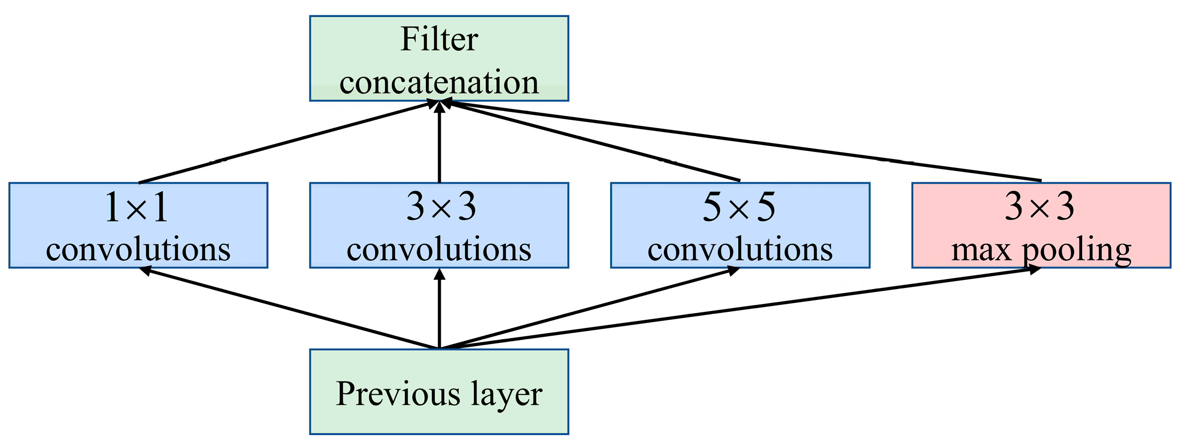
2.2. Inception Module

The main idea of the inception model, introduced by Szegedy et al. [27], is to consider how an optimal local sparse structure of a convolutional vision network can be replaced by dense matrix operations. The inception module has three sizes of convolutional kernels: 1 × 1 , 3 × 3 , 5 × 5 , as shown in Figure 1. Convolution kernels of different sizes ensure the acquisition of multi-scale features. In addition, the addition of the pooling operation also further improves the model’s performance. Compared with the traditional convolutional model, the inception model has a stronger feature extraction capability, thus greatly improving the model’s performance.

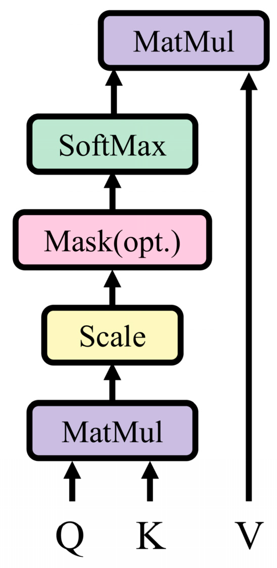
2.3. Scaled Dot-Product Attention

The attention mechanism helps the network model to assign different weights to each part of the input so that more critical information can be extracted, thus improving the performance of the model. As a variant of the attention mechanism, the self-attention mechanism reduces the reliance on external information and is better at capturing the internal relevance of data or features. Scaled dot-product attention is the basic form of the self-attention mechanism proposed by Vaswani et al. [28]. It calculates the responses for each position in the sequence by estimating the attention scores for all positions and collecting the corresponding inputs based on the scores, as shown in Figure 2. The calculation process is as follows:
Q = W q · X K = W k · X V = W v · X
Y = S A ( Q , K , V ) = s o f t m a x ( A ) · V = s o f t m a x Q · K T d · V
where X = x 1 , x 2 , , x n n × d is the input, n is the sequence length, d is the number of dimensions, W q , W k , W v d × d are the three different linear transformation matrices, Q ,   K ,   V d × d are the three intermediate matrices, S A ( · ) represents the self-attention calculation, A n × n is the self-attention matrix, and each element in A represents the attention fraction between two elements in X . s o f t m a x · is the softmax operation, and Y = y 1 , y 2 , , y n n × d is the final output sequence.

2.4. Mutual Information

Mutual Information is a useful information measure in information theory, referring to the degree of correlation between two random variables, i.e., the degree to which the uncertainty of one random variable is diminished when another random variable is determined. Formally, the mutual information of two discrete random variables X and Y can be defined as
I ( X ; Y ) = y Y x X p ( x , y ) log p ( x , y ) p ( x ) p ( y )
In the case of continuous random variables, the summation is replaced by a dual definite integral in the form of
I ( X ; Y ) = Y X p ( x , y ) log p ( x , y ) p ( x ) p ( y ) d x d y
where p ( x , y ) is the joint probability density function of X and Y, and p ( x ) , p ( y ) are the marginal probability density functions of X and Y, respectively. The mutual information takes the minimum value of 0, which means that given one random variable has no relationship with another random variable, the maximum value is the entropy of the random variable, which means that given one random variable, the uncertainty of the other random variable can be completely eliminated.

3. Proposed Method

In this study, we propose an improved method, MMDCNN, based on 1D_CNN that can diagnose rolling bearings under interference environments. Firstly, a multi-scale feature extractor was designed to enrich the fault information and enhance the effective features adaptively. Secondly, unsupervised mutual information loss was added to the supervised cross-entropy loss; thus, the proposed method can extract robust fault features with high generalization performance.

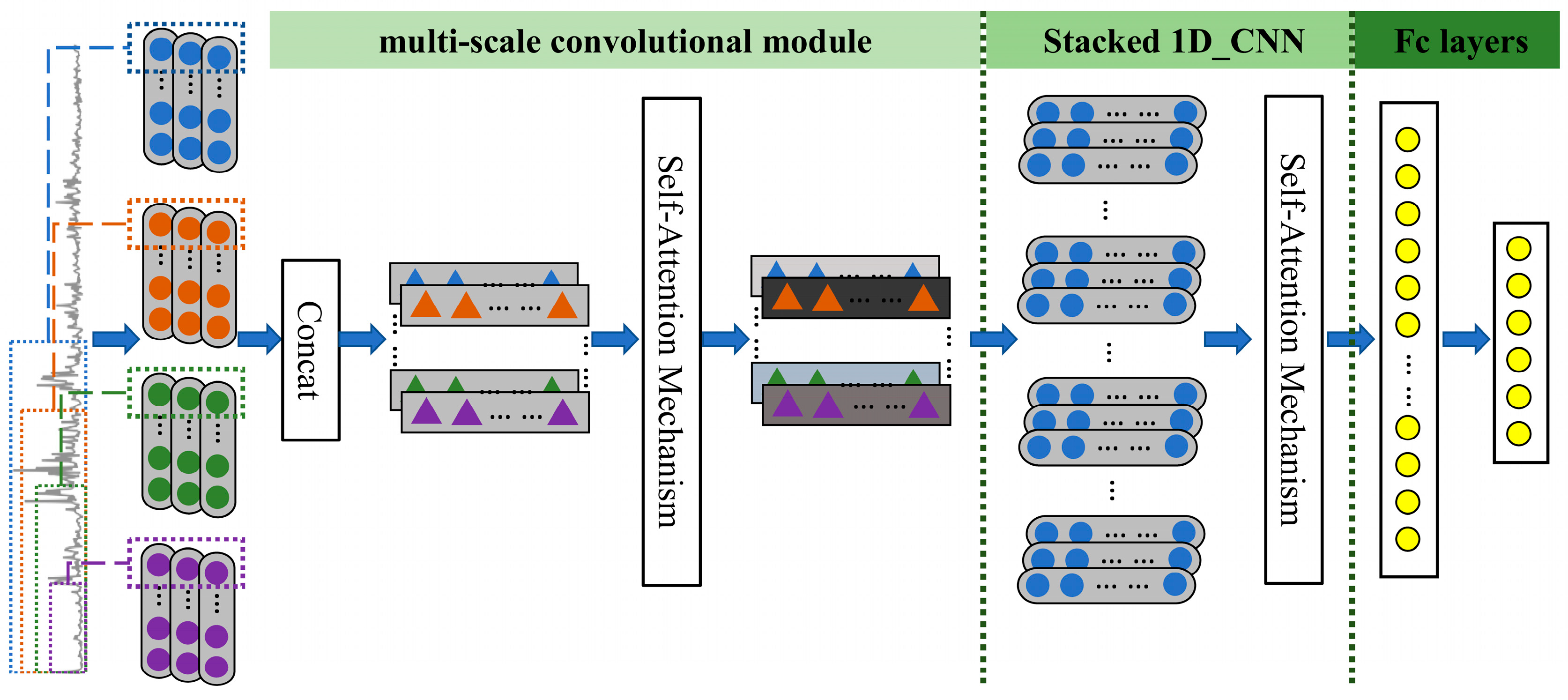
3.1. Multi-Scale Feature Extraction Network

In convolutional feature extractors, single-scale representations with fixed convolutional kernels may lose critical information needed to further enhance the performance. The inception module successfully improves the model’s performance by maximizing feature diversity through substructures with different receptive field sizes, adopting a multi-scale perspective. Inspired by the inception module, this paper proposes a multi-scale feature extraction network. As shown in Figure 3, the network architecture consists of three components. In the multi-scale convolution module, multi-scale convolution layers are positioned at the forefront of the model to maximize the retention of initial features that encompass multidimensional fault information. Subsequently, a self-attention mechanism is introduced to adaptively enhance the key fault information within the multi-scale initial features. Following this, the network’s expressiveness is improved by deepening it through the stacked 1D_CNN module, which adds subsequent layers of single-scale small convolution kernels. Additionally, a self-attention mechanism is applied again to adaptively weigh and enhance high-level abstract features. Finally, the fully connected layer performs the final fault classification.
Specifically, the specific process of the multi-scale convolution module is as follows: the input data are convolved in parallel by a convolution layer with 1 × 1 , 1 × 3 , 1 × 5 , and 1 × 7 convolution kernels; the total number of channels is 48. The convolution process uses zero padding, batch normalization, and the ReLu activation function. In addition, a maximum pooling layer of size 2 and step size of 2 are added after the convolution layer to reduce the feature dimensionality. Finally, the feature dimensions of different branches are stacked and stitched together by the concat operation. The detailed architectural parameters of the network are shown in Table 1.

3.2. Composite Loss Function Construction

Considering the existence of redundant environmental information shared among categories, it is difficult to extract pure fault features by relying on feature extractors alone. Therefore, it is often difficult to achieve the desired effect with cross-entropy loss, resulting in some samples that may have similar probabilities at different label positions, as shown in Figure 4. To improve this problem, the concept of mutual information is introduced in this paper. The mutual information between the faulty samples and the corresponding features can be used to measure the uniqueness of the features extracted from the samples. The enhancement of mutual information implies that the redundant environmental information shared between heterogeneous features is weakened, i.e., the proportion of true fault information is elevated. Therefore, we propose a new composite loss function method that combines cross-entropy loss and mutual information loss. By maximizing the mutual information, the fault feature extraction capability of the model is further improved.
The direct optimization of mutual information is usually difficult to operate, especially in the form of neural networks, so the idea of the DEEP INFOMAX(DIM) model proposed by Hjelm et al. [29] is adopted in this paper. As an unsupervised learning model, the DIM model trains an encoder to maximize the mutual information between its inputs and outputs and achieves better performance than many popular unsupervised learning methods. In the DIM model, Equation (7) is converted as follows:
p ( z x ) = min p ( z x ) , T ( x , z ) { β · ( E ( x , z ) p ( z x ) p ( x ) [ log σ ( T ( x , z ) ) ] + E ( x , z ) p ( z ) p ( x ) [ log ( 1 σ ( T ( x , z ) ) ) ] ) + γ · E x p ( x ) [ K L ( p ( z x ) q ( z ) ) ] }
where x X denotes a single sample in the set of inputs, z Z denotes an individual feature vector in the set of abstract feature vectors, and p ( z x ) denotes the distribution of the feature vector generated by x . σ ( T ( x , z ) ) represents a discriminant network, which is used for “negative sampling estimation”, i.e., where the input signal sample x and the corresponding feature vector z can be considered as positive sample pairs, and x and randomly shuffled z can be considered as negative sample pairs. q ( z ) is the standard normal distribution, which is used to make the feature space more regular, thus facilitating model training. β ,   γ are hyperparameters.
Based on the idea of the DIM model, this paper merges the mutual information loss based on the cross-entropy loss function. The composite loss function network in this paper is shown in Figure 5. First, the cross-entropy loss is calculated and named L y . Assume that the input of a batch is X = x 1 , x 2 , , x n n × d , where n is the number of samples and d is the length of a single sample. According to the VAE model [30], the final convolutional feature maps obtained by the stacked 1D_ CNN are globally pooled and fed into the encoders (FC_VAE_1, FC_VAE_2) to obtain the mean μ and variance σ 2 , respectively; thus, the scatter loss of the prior distribution can be calculated, which is denoted as L k l . Then, the encoded feature vectors Z = z 1 , z 2 , z 3 , , z n n × k can be obtained, where k is the number of convolutional feature maps. x i , z i | i = 1 , 2 , , n can constitute positive sample pairs, while x ˜ i , z i | i = 1 , 2 , , n represents a negative sample pair, where X and Z are randomly shuffled and reorganized as X ˜ and Z ˜ , respectively. To simplify the calculations, the positive and negative sample pairs can then be simplified separately as z i , z i | i = 1 , 2 , , n and z ˜ i , z i | i = 1 , 2 , , n . A four-layer fully connected network is designed as the discriminatory network σ ( T ( x , z ) ) . Considering that the intermediate convolutional feature maps contain more fault information, the intermediate convolutional feature maps are further selected to form sample pairs with the final convolutional feature maps. The feature maps of the middle convolutional layer are selected and denoted as C = c 1 , c 2 , c 3 , , c n n × w × c , where n is the number of samples, and ω × c represents the feature dimension. Expanding Z to the same dimension as C , c i , z i | i = 1 , 2 , , n can be viewed as positive sample pairs and, relatively, c ˜ i , z i | i = 1 , 2 , , n can be taken as negative sample pairs. The network form of σ ( T ( c , z ) ) remains the same as σ ( T ( x , z ) ) ; thus, L L and L G can be calculated. All the specific structural parameters are shown in Table 1. Based on Equation (8), the optimization objective J based on the composite loss function can be rewritten as follows, where α ,   β ,   ε ,   γ are hyperparameters:
J = min { L y + α · ( β · L G ε · L L + γ · L k l ) } = min { L y + α · ( β · ( E [ log σ ( T ( z i , z i ) ) ] + E [ log ( 1 σ ( T ( z ˜ i , z i ) ) ) ] ) ε · ( E [ log σ ( T ( c i , z i ) ) ] + E [ log ( 1 σ ( T ( c ˜ i , z i ) ) ) ] ) + γ · L k l ) }

4. Experimental Validation and Analysis

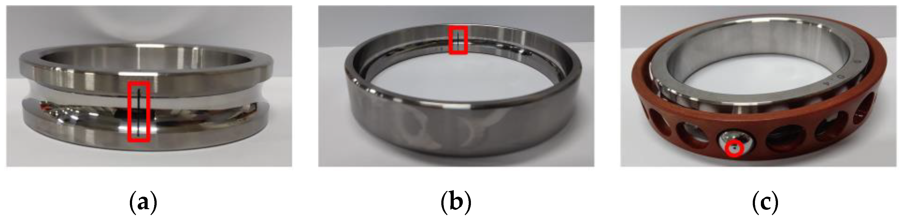
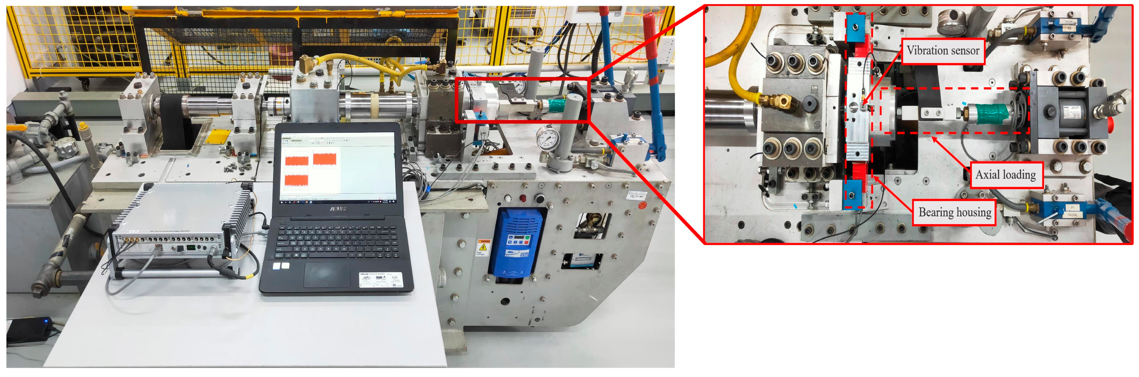
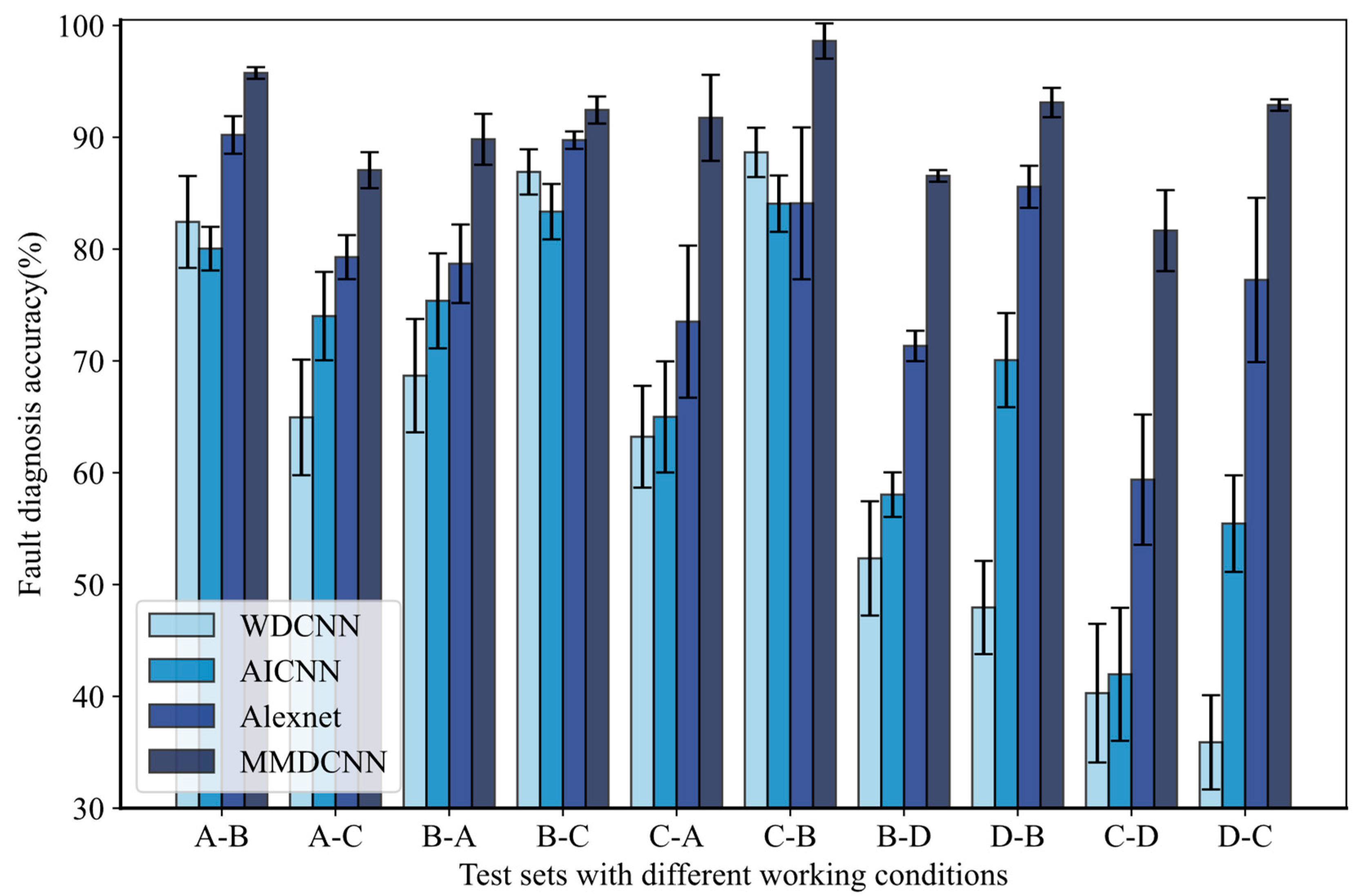
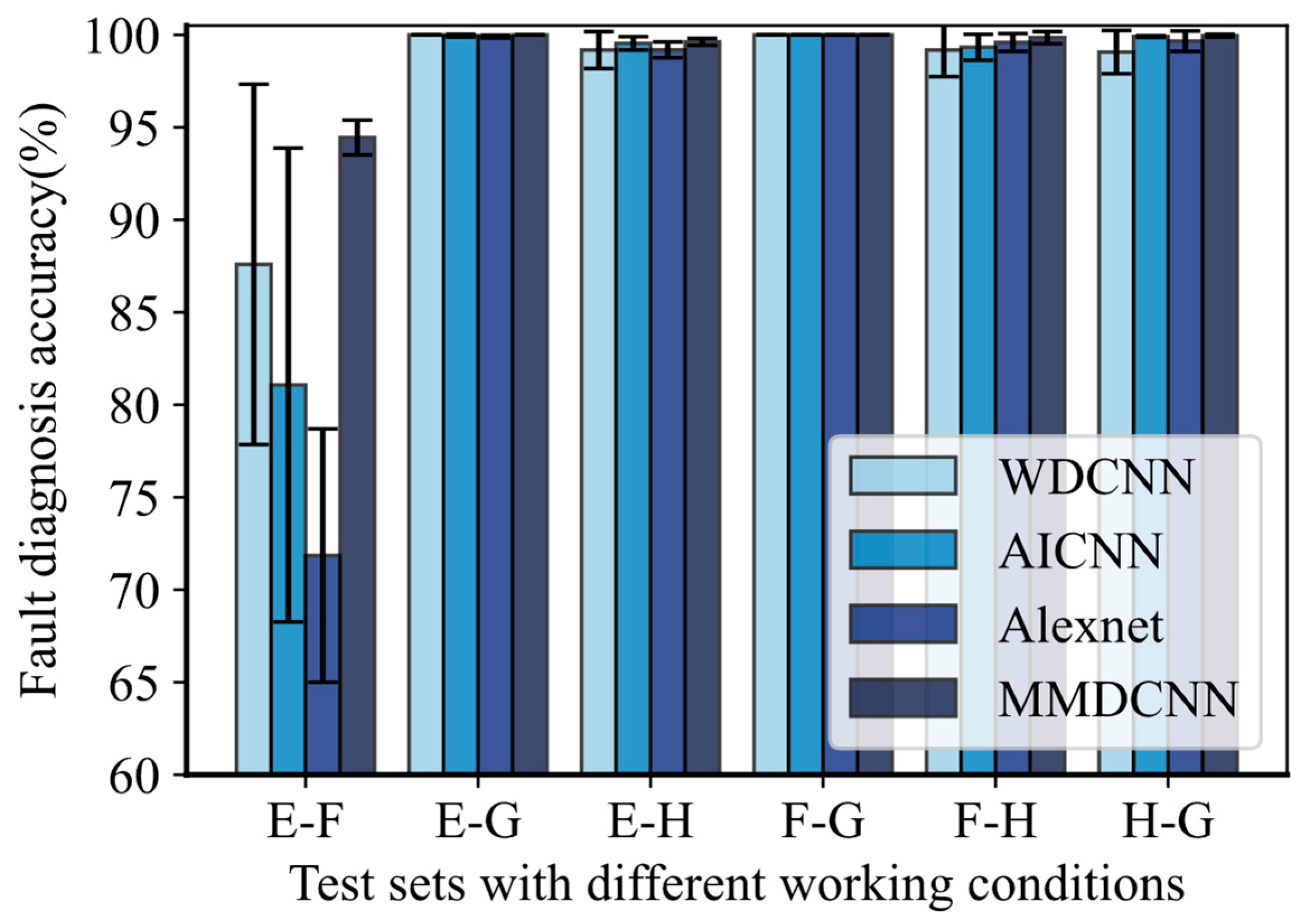
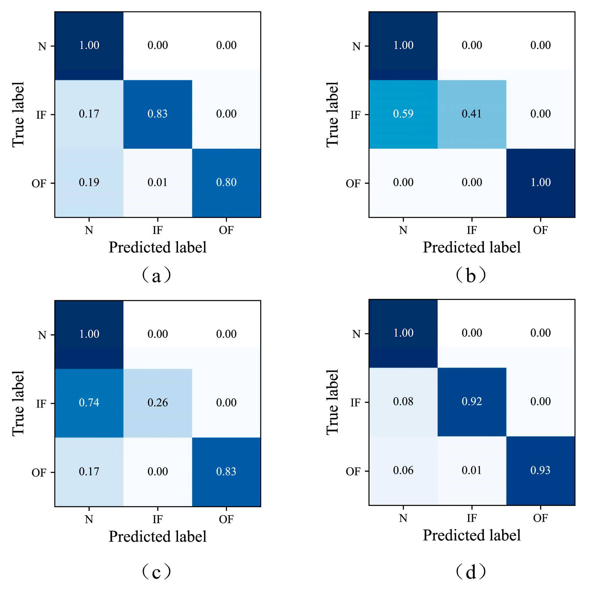
4.1. Case 1: Experiments on Spindle Bearing Simulation Fault Dataset

To verify the validity of the proposed model, the spindle bearing simulation fault dataset was adopted first. The bearing code was 7014AC, and ten health conditions (N, BF, IF, and 12 o’clock OF) with (0.4, 0.6, 0.8) mm artificial faults were used. The different forms of the bearing failures are shown in Figure 6. The BPS test bench was selected as the test platform. The motor drives the spindle rotation through the belt, and the bearing housing receives the axial load from the hydraulic rod, as shown in Figure 7. A vibration sensor collects the vibration data at a sampling frequency of 32 kHz. Two speeds (1500/2100 r/min) and three axial loads (1/2/3 kN) were set to simulate different working conditions. Depending on the differences in working conditions, datasets were established, as shown in Table 2. Each dataset included 6000 samples of 2048 points and was enhanced by sliding window overlapping sampling (overlapping rate is 0.5). A total of 70% of the samples in each dataset were used for training and the rest for testing. To verify that the proposed method has a strong fault feature extraction capability, the model training set and the test set were from datasets with different working conditions. For example, A–D represents the training set from dataset A and the test set from dataset D.
The structural parameters of MMDCNN are shown in Table 1. The training process adopted an Adam optimizer with a training batch size of 256 and a learning rate of 0.001. The super parameters were selected as α = 0.01 ,   β = 0.5 ,   ε = 1.5 ,   γ = 0.05 after many tests. The number of iterative training epochs of the model was 30 epochs. In addition, the Alexnet model [31], the WDCNN model proposed by Zhang et al. [32], and the AICNN model proposed by Zhu et al. [24] were selected for comparison to prove the advantages of the proposed method. The convolution depths of the three compared models were consistent with the proposed model for a fair comparison. To avoid the effect of model parameter initialization, all models were trained ten times randomly. The mean and standard deviation of the diagnostic accuracy of the ten tests were used as the evaluation index. The experimental results are shown in Figure 8.
It can be seen from Figure 8 that the proposed method performed significantly better than the comparison methods. On the tasks with load fluctuations, the average fault diagnosis accuracy of MMDCNN reached 92.57%. Especially in the case of C-A, MMDCNN achieved an accuracy of 91.74%, outperforming the comparison models by nearly 18~28%. On the tasks with speed fluctuations, the average fault diagnosis accuracy of MMDCNN reached 89.83%, which was able to meet the demand for fault diagnosis. More importantly, it can be seen that the proposed method could still achieve a high diagnosis accuracy of 87.27% on the tasks with significant fluctuations in both speed and load, while Alexnet could only reach 68.31%.
In summary, it can be seen that the average diagnostic performance of the proposed model decreased slightly as the difficulty of the diagnostic task increased, but the comparison methods greatly lost their diagnostic capability. One of the reasons is the addition of the first multi-scale convolution layer and the self-attention mechanisms in MMDCNN, so that multi-scale features containing more effective fault features are adaptively enhanced. Another main reason is that the difference in convolutional features belonging to different health conditions is maximized due to mutual information loss; thus, the proposed method can extract robust fault features with high generalization performance. In addition, it was found that when compared to other methods, MMDCNN displayed the smallest standard deviation of multiple tests. This may also demonstrate the effect of mutual information. As for the comparison methods, the model inputs varied tremendously due to fluctuations in the working conditions. Alexnet as well as WDCNN performed poorly due to the lack of multi-scale convolution. In addition, the setting of the first layer with a wide convolution kernel in WDCNN may have made it difficult to capture critical details in the spectrum. Although AICNN introduces the inception structure, the front end is a single-scale convolution layer; thus, some critical information may have been lost. In addition, the disadvantage of the cross-entropy loss function caused large standard deviations for the multiple testing of all the compared models, which further limited the overall feature extraction ability of the models.
In order to further analyze the experimental results, the confusion matrices of the training results on tasks C-D/D-C are given in Figure 9. As can be seen from Figure 9, MMDCNN achieved an almost 100% diagnostic accuracy for the four major fault categories (N/OF/IF/BF). The proposed method achieved good discrimination for the inner and outer loop faults, except for the confusion in the discrimination of the outer loop fault degree on the C-D task. In addition, the proposed method was also significantly better than the comparison methods for diagnosing ball faults with different failure degrees, especially in BF_1 and BF_2.
As mentioned above, the proposed method is able to resist the interference caused by fluctuations in working conditions. However, the noise intensity also constantly changes during machinery operation, and the interference caused by it also greatly affects the performance of the diagnostic model. To explore the performance of MMDCNN under unknown noise conditions, we trained the network with dataset D under S N R dB = 0   dB and then tested the model under S N R dB = 2   dB and S N R dB = 2   dB , respectively. The experimental results are shown in Figure 10.
As can be seen from Figure 10, the proposed method performed the best among all the methods and had a more stable test performance. It is worth noting that the performance of AICNN was closer to that of MMDCNN. Considering the addition of the inception module in AICNN, the effect of multi-scale convolution can be demonstrated. However, the standard deviation of MMDCNN was smaller compared to AICNN, which may reflect the role of mutual information loss. Similarly, in order to probe the role of each part of MMDCNN under varying noise, another ablation experiment was conducted. The experimental results were consistent with those under changing work conditions, which are given in Table A1 in Appendix A.

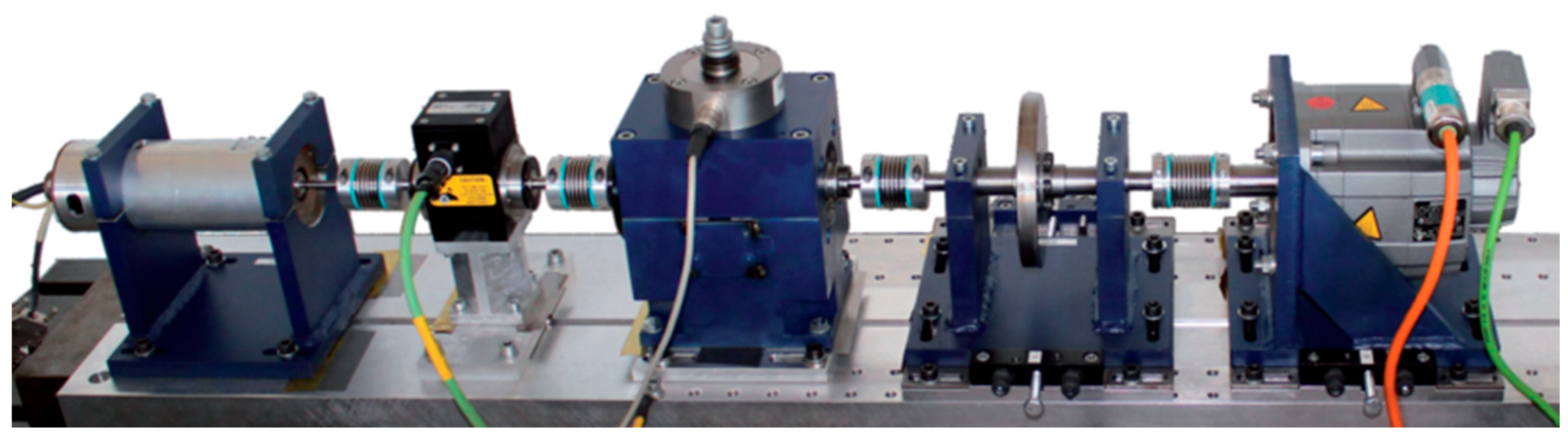
4.2. Case 2: Experiments on the Paderborn University (PU) Dataset

To further validate the practicality of the proposed method, real bearing damage data from Paderborn University (PU) were selected for further validation experiments [33]. These real bearing damage samples were generated by accelerated lifetime tests, which are closer to actual failure scenarios than artificial damages. The equipment platform is shown in Figure 11. The sampling frequency was 64 kHz. Three health conditions (N, IF, OF) from bearings (K004, KI21, KA04) were used. The PU dataset consists of four working conditions, namely (1500, 0.7, 1000), (900, 0.7, 1000), (1500, 0.1, 1000), and (1500, 0.7, 0.4), where the elements refer to speed (rpm), torque (N·m), and radial load (N), respectively. Therefore, four types of datasets (dataset E/F/G/H) were named sequentially according to the working conditions mentioned above.
The parameter settings of the datasets and MMDCNN remained unchanged. Firstly, we verified the feature extraction performance of the model under fluctuating working conditions. As can be seen from Figure 12, the proposed method outperformed or equaled the comparison methods for all tasks. In addition, MMDCNN performed more consistently, which corroborates the analysis in Case 2. It is worth noting the large differences in diagnostic accuracy between the methods on task E-F. The reduction in rotational speed clearly posed a great challenge to the generalization performance of the diagnostic model, which can also be observed in Case 2. To further probe the reason for this decrease in accuracy, the average confusion matrices of the training results on task E-F are given in Figure 13.
As can be seen in Figure 13, the high miss rate of the inner and outer ring fault samples resulted in a decrease in the accuracy of these diagnostic models. Especially for the inner ring samples, the average diagnostic accuracy of the three comparison methods was only 50%, while the proposed method could reach 92%. The confusion matrix shows that the fault state was indistinguishable from the normal state, which means that the comparison models could not extract fault features under the fluctuating working conditions. Considering that all of the comparison methods easily achieved 100% diagnostic accuracy during training, the accuracy dropped dramatically during testing. The reason can only be the poor fault feature extraction ability of the comparison models, which makes it difficult to discover the most fundamental fault features when the input distribution changes. However, the proposed method greatly enhanced the effective fault mining capability by adding the first multi-scale convolutional layer and the self-attention mechanism. In addition, the generalization performance and robustness of the extracted fault features were further enhanced due to the addition of mutual information loss. Therefore, the proposed method could still maintain good diagnostic accuracy.
Similarly, experiments under varying noise on the PU dataset were also conducted. Considering that there were only three categories, the degree of noise was increased accordingly. Dataset E under S N R dB = 4   dB was selected for training and then tested with S N R dB = 8   dB and S N R dB = 0   dB . The experimental results were consistent with Case 1, which are also given in Figure A1 in Appendix B.

4.3. Ablation Experiments

To verify the importance of each part of the model, an ablation study was conducted on task D-C. By removing each part of the model in turn, the degree of their contribution could be observed. The test results are shown in Table 3.
As can be seen from Table 3, the average diagnostic accuracy was improved by nearly 12% due to the addition of multi-scale convolution. There is no doubt that the combination of the self-attentive mechanism and multi-scale convolution greatly improved the model fault feature extraction capability. However, the presence of redundant environmental information in the multiscale features led to less stable test results. The addition of mutual information loss resulted in a 4% improvement in accuracy, while the standard deviation for multiple tests decreased significantly. In this way, we can assume that the addition of mutual information loss enhanced the robustness and generalization performance of the fault features. However, the lack of multi-scale convolution led to a decrease in the overall feature extraction ability of the network. In summary, all parts of the proposed method are useful for the improvement of the overall diagnosis accuracy.

4.4. Computational Cost Analysis

To further assess the practical applicability of the proposed method in real industrial scenarios, a time consumption analysis was conducted for both the proposed method and the comparison methods. All training and testing were performed on a single NVIDIA 1050Ti GPU. The final results are shown in Table 4. It can be observed that the proposed method required the longest training time per epoch among all the methods, averaging 2.39 s. However, in terms of the testing time, the inference time for all the methods was 0.0001 s when rounded to four decimal places. This is because the additional mutual information module in the proposed model is only involved in the training optimization process and does not participate in the inference process. Currently, in industrial environments, models are typically trained in the cloud and then deployed to edge devices. Given that the proposed method achieved the best generalization performance with the same inference time, it can be considered to have practical industrial application value.

5. Conclusions

In the paper, an improved convolutional bearing fault diagnosis model named MMDCNN with a strong feature extraction capability is proposed. Firstly, a multi-scale feature extraction layer located at the front end of the model guarantees the comprehensive extraction of initial feature information. Then, a self-attention mechanism is applied to adaptively enhance the critical fault components in the multi-scale features. Finally, the generalization performance and robustness of the critical fault features are further enhanced by compounding mutual information loss based on cross-entropy loss. By using the above three methodologies, the strong feature extraction capability of MMDCNN under interference environments is guaranteed. To demonstrate the advantages of the proposed method, three datasets were used. The results showed that MMDCNN performed significantly better than other diagnostic frameworks in both fluctuating working conditions and noisy environments. The analysis of the above results indicates that the method has good application prospects for the diagnosis of bearings in actual industrial scenes.

Author Contributions

Conceptualization, K.H.; Methodology, K.H. and L.Z. (Linbo Zhu); Validation, K.H.; Formal analysis, L.Z. (Linbo Zhu) and Z.R.; Resources, L.Z. (Linbo Zhu) and Y.Z.; Data curation, K.H., Z.R. and T.L.; Writing—original draft, K.H.; Writing—review & editing, K.H., L.Z. (Linbo Zhu), Z.R., T.L. and Y.Z.; Visualization, K.H.; Supervision, L.Z. (Linbo Zhu), L.Z. (Li Zeng), J.W. and Y.Z.; Project administration, L.Z. (Linbo Zhu), L.Z. (Li Zeng), J.W. and Y.Z.; Funding acquisition, L.Z. (Linbo Zhu), L.Z. (Li Zeng) and J.W. All authors have read and agreed to the published version of the manuscript.

Funding

This research was supported by the Xi’an Science and Technology Planning Project—Key Industry Chain Application Scenario Demonstration Project—Research and Performance Study of Efficient and Energy-Saving Intelligent Permanent Magnet Traction System (project number: 23ZDCYYYCJ0007).

Data Availability Statement

The data presented in this study are available on request from the corresponding author.

Conflicts of Interest

Author Li Zeng and Author Jin Wan are employed by the company CRRC Xi’an YongeJieTong Electric Co., Ltd. The remaining authors declare that the research was conducted in the absence of any commercial or financial relationships that could be construed as a potential conflict of interest.

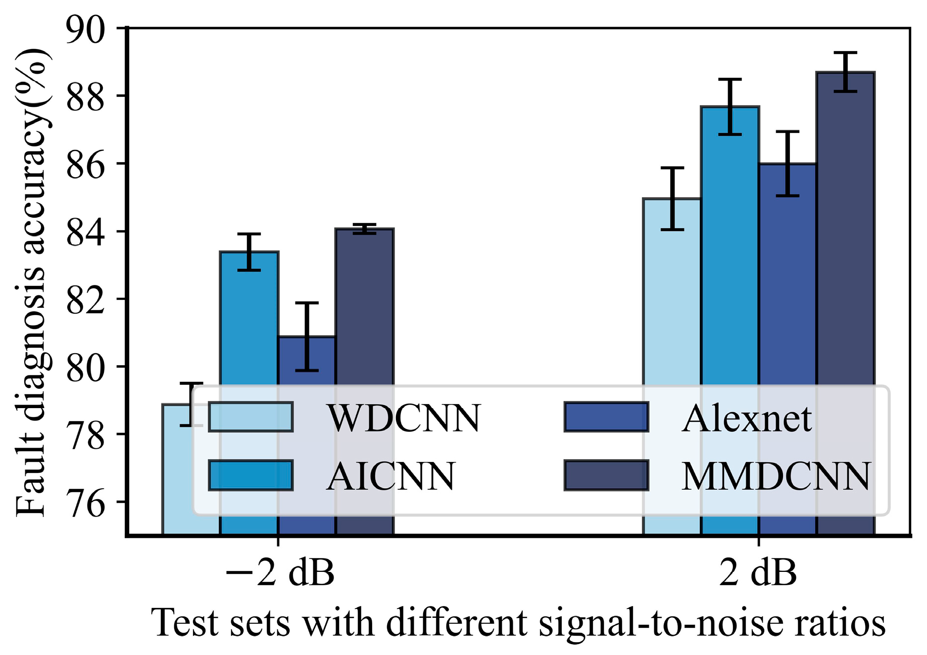
Appendix A. The Ablation Study on Dataset D under Varying Noise

Table A1. The ablation study on dataset D under varying noise.
MethodsAccuracy (%)
SNR = 0 dB
SNR = −2 dBSNR = 2 dB
MMDCNN without multi-scale convolution part82.61 ± 0.6287.33 ± 0.44
MMDCNN without mutual information part83.33 ± 0.8387.66 ± 0.62
MMDCNN without all contributive parts80.88 ± 1.0085.99 ± 0.95
MMDCNN84.07 ± 0.1388.70 ± 0.58

Appendix B. The Comparison Experiment on Dataset E under Varying Noise

Figure A1. Comparison of fault diagnosis results under varying noise.
Machines 12 00383 g0a1

References

  1. Wang, H.; Xu, J.; Yan, R.; Gao, R.X. A New Intelligent Bearing Fault Diagnosis Method Using SDP Representation and SE-CNN. IEEE Trans. Instrum. Meas. 2020, 69, 52377–52389. [Google Scholar] [CrossRef]
  2. Gao, D.; Huang, K.; Zhu, Y.; Zhu, L.; Yan, K.; Ren, Z.; Soares, C.G. Semi-supervised small sample fault diagnosis under a wide range of speed variation conditions based on uncertainty analysis. Reliab. Eng. Syst. Saf. 2024, 242, 109746. [Google Scholar] [CrossRef]
  3. Wang, X.; Shen, C.; Xia, M.; Wang, D.; Zhu, J.; Zhu, Z. Multi-scale deep intra-class transfer learning for bearing fault diagnosis. Reliab. Eng. Syst. Saf. 2020, 202, 107050. [Google Scholar] [CrossRef]
  4. Gao, H.; Liang, L.; Chen, X.; Xu, G. Feature extraction and recognition for rolling element bearing fault utilizing short-time Fourier transform and non-negative matrix factorization. Chin. J. Mech. Eng. 2015, 28, 96–105. [Google Scholar] [CrossRef]
  5. Dybała, J.; Zimroz, R. Rolling bearing diagnosing method based on empirical mode decomposition of machine vibration signal. Appl. Acoust. 2014, 77, 195–203. [Google Scholar] [CrossRef]
  6. Wang, D.; Kwok-Leung, T.; Yong, Q. Optimization of segmentation fragments in empirical wavelet transform and its applications to extracting industrial bearing fault features. Measurement 2019, 133, 328–340. [Google Scholar] [CrossRef]
  7. Yu, J. Local and nonlocal preserving projection for bearing defect classification and performance assessment. IEEE Trans. Ind. Electron. 2011, 59, 2363–2376. [Google Scholar] [CrossRef]
  8. Soualhi, A.; Kamal, M.; Noureddine, Z. Bearing health monitoring based on Hilbert–Huang transform, support vector machine, and regression. IEEE Trans. Instrum. Meas. 2014, 64, 52–62. [Google Scholar] [CrossRef]
  9. Yu, W.; Zhao, C. Robust monitoring and fault isolation of nonlinear industrial processes using denoising autoencoder and elastic net. IEEE Trans. Control Syst. Technol. 2019, 28, 1083–1091. [Google Scholar] [CrossRef]
  10. Yu, W.; Zhao, C.; Huang, B. MoniNet with concurrent analytics of temporal and spatial information for fault detection in industrial processes. IEEE Trans. Cybern. 2021, 52, 8340–8351. [Google Scholar] [CrossRef]
  11. LeCun, Y.; Boser, B.; Denker, J.S.; Henderson, D.; Howard, R.E.; Hubbard, W.; Jackel, L.D. Backpropagation applied to handwritten zip code recognition. Neural Comput. 1989, 1, 541–551. [Google Scholar] [CrossRef]
  12. Long, Y.; Zhou, W.; Luo, Y. A fault diagnosis method based on one-dimensional data enhancement and convolutional neural network. Measurement 2021, 180, 109532. [Google Scholar] [CrossRef]
  13. Wen, L.; Li, X.; Gao, L.; Zhang, Y. A new convolutional neural network-based data-driven fault diagnosis method. IEEE Trans. Ind. Electron. 2017, 65, 5990–5998. [Google Scholar] [CrossRef]
  14. Chen, H.; Hu, N.; Cheng, Z.; Zhang, L.; Zhang, Y. A deep convolutional neural network based fusion method of two-direction vibration signal data for health state identification of planetary gearboxes. Measurement 2019, 146, 268–278. [Google Scholar] [CrossRef]
  15. He, Z.; Shao, H.; Zhong, X.; Zhao, X. Ensemble transfer CNNs driven by multi-channel signals for fault diagnosis of rotating machinery cross working conditions. Knowl.-Based Syst. 2020, 207, 106396. [Google Scholar] [CrossRef]
  16. Yu, W.; Zhao, C. Broad convolutional neural network based industrial process fault diagnosis with incremental learning capability. IEEE Trans. Ind. Electron. 2019, 67, 5081–5091. [Google Scholar] [CrossRef]
  17. Huo, C.; Jiang, Q.; Shen, Y.; Zhu, Q.; Zhang, Q. Enhanced transfer learning method for rolling bearing fault diagnosis based on linear superposition network. Eng. Appl. Artif. Intell. 2023, 121, 105970. [Google Scholar] [CrossRef]
  18. Tang, G.; Yi, C.; Liu, L.; Xu, D.; Zhou, Q.; Hu, Y.; Zhou, P.; Lin, J. A parallel ensemble optimization and transfer learning based intelligent fault diagnosis framework for bearings. Eng. Appl. Artif. Intell. 2024, 127, 107407. [Google Scholar] [CrossRef]
  19. Ganin, Y.; Ustinova, E.; Ajakan, H.; Germain, P.; Larochelle, H.; Laviolette, F.; March, M.; Lempitsky, V. Domain-Adversarial Training of Neural Networks. In Domain Adaptation in Computer Vision Applications; Advances in Computer Vision and Pattern Recognition; Csurka, G., Ed.; Springer International Publishing: Cham, Switzerland, 2017; pp. 189–209. [Google Scholar] [CrossRef]
  20. Wang, Y.-Q.; Zhao, Y.-P. A novel inter-domain attention-based adversarial network for aero-engine partial unsupervised cross-domain fault diagnosis. Eng. Appl. Artif. Intell. 2023, 123, 106486. [Google Scholar] [CrossRef]
  21. Ren, H.; Wang, J.; Zhu, Z.; Shi, J.; Huang, W. Domain fuzzy generalization networks for semi-supervised intelligent fault diagnosis under unseen working conditions. Mech. Syst. Signal Process. 2023, 200, 110579. [Google Scholar] [CrossRef]
  22. Chen, L.; Li, Q.; Shen, C.; Zhu, J.; Wang, D.; Xia, M. Adversarial Domain-Invariant Generalization: A Generic Domain-Regressive Framework for Bearing Fault Diagnosis Under Unseen Conditions. IEEE Trans. Ind. Inform. 2022, 18, 31790–31800. [Google Scholar] [CrossRef]
  23. Zhao, C.; Shen, W. Mutual-assistance semisupervised domain generalization network for intelligent fault diagnosis under unseen working conditions. Mech. Syst. Signal Process. 2023, 189, 110074. [Google Scholar] [CrossRef]
  24. Zhu, H.; Ning, Q.; Lei, Y.J.; Chen, B.C.; Yan, H. Rolling bearing fault classification based on attention mechanism-Inception-CNN model. J. Vib. Shock 2020, 39, 84–93. [Google Scholar]
  25. Zhang, K.; Wang, J.; Shi, H.; Zhang, X.; Tang, Y. A fault diagnosis method based on improved convolutional neural network for bearings under variable working conditions. Measurement 2021, 182, 109749. [Google Scholar] [CrossRef]
  26. Li, S.; An, Z.; Lu, J. A novel data-driven fault feature separation method and its application on intelligent fault diagnosis under variable working conditions. IEEE Access 2020, 8, 113702–113712. [Google Scholar] [CrossRef]
  27. Szegedy, C.; Liu, W.; Jia, Y.; Sermanet, P.; Reed, S.; Anguelov, D.; Erhan, D.; Vanhoucke, V.; Rabinovich, A. Going deeper with convolutions. In Proceedings of the IEEE Conference on Computer Vision and Pattern Recognition, Boston, MA, USA, 7–12 June 2015. [Google Scholar]
  28. Vaswani, A.; Shazeer, N.; Parmar, N.; Uszkoreit, J.; Jones, L.; Gomez, A.N.; Kaiser, Ł.; Polosukhin, I. Attention is all you need. In Proceedings of the Annual Conference on Neural Information Processing Systems 2017, Long Beach, CA, USA, 4–9 December 2017. [Google Scholar]
  29. Hjelm, R.D.; Fedorov, A.; Lavoie-Marchildon, S.; Grewal, K.; Bachman, P.; Trischler, A.; Bengio, Y. Learning deep representations by mutual information estimation and maximization. arXiv 2018, arXiv:1808.06670. [Google Scholar]
  30. Kingma, D.P.; Welling, M. Auto-encoding variational bayes. arXiv 2013, arXiv:1312.6114. [Google Scholar]
  31. Krizhevsky, A.; Sutskever, I.; Hinton, G.E. Imagenet classification with deep convolutional neural networks. Adv. Neural Inf. Process. Syst. 2012, 25, 1097–1105. [Google Scholar] [CrossRef]
  32. Zhang, W.; Peng, G.; Li, C.; Chen, Y.; Zhang, Z. A new deep learning model for fault diagnosis with good anti-noise and domain adaptation ability on raw vibration signals. Sensors 2017, 17, 425. [Google Scholar] [CrossRef]
  33. Lessmeier, C.; Kimotho, J.K.; Zimmer, D.; Sextro, W. Kat-Datacenter, Chair of Design and Drive Technology. Paderborn University. Available online: https://mb.uni-paderborn.de/kat/forschung/kat-datacenter/bearing-datacenter (accessed on 27 May 2024).
Figure 1. Inception module.
Machines 12 00383 g001
Figure 2. Scaled dot-product attention.
Machines 12 00383 g002
Figure 3. Basic architecture of feature extraction method.
Machines 12 00383 g003
Figure 4. Comparison of cross-entropy loss and composite loss.
Machines 12 00383 g004
Figure 5. Model architecture of MMDCNN.
Machines 12 00383 g005
Figure 6. 7014Ac bearing with different faults: (a) outer ring fault, (b) inner ring fault, (c) ball fault.
Machines 12 00383 g006
Figure 7. Spindle bearing test platform.
Machines 12 00383 g007
Figure 8. Comparison of fault diagnosis results on different tasks.
Machines 12 00383 g008
Figure 9. Confusion matrix on spindle bearing simulation fault dataset: (a) MMDCNN (task: C-D), (b) Alexnet (task: C-D), (c) MMDCNN (task: D-C), (d) Alexnet (task: D-C).
Machines 12 00383 g009
Figure 10. Comparison of fault diagnosis results under varying noise.
Machines 12 00383 g010
Figure 11. The platform of the PU bearing dataset.
Machines 12 00383 g011
Figure 12. Comparison of fault diagnosis results on different tasks.
Machines 12 00383 g012
Figure 13. Average confusion matrix on task E-F of PU dataset: (a) WDCNN, (b) AICNN, (c) Alexnet, (d) MMDCNN.
Machines 12 00383 g013
Table 1. Architecture parameters of the MMDCNN.
TypeLayerKernel Size/Stride/DepthInput SizeOutput Size
Multi-scale feature
convolutional module
Inception N(N/2, 48)
Self-attention mechanism (N/2, 48)(N/2, 48)
Conv Module1Convolution3/1/64
(Zero padding)
(N/2, 48)(N/4, 64)
BN/
Max Pooling2/2/64
Conv Module2Convolution3/1/64
(Zero padding)
(N/4, 64)(N/8, 64)
BN/
Max Pooling2/2/64
Conv Module3Convolution3/1/64
(Zero padding)
(N/8, 64)(N/16, 64)
BN/
Max Pooling2/2/64
Conv Module4Convolution3/1/64(N/16, 64)((N/16 − 2)/2, 64)
BN/
Max Pooling2/2/64
Self-attention mechanism ((N/16 − 2)/2, 64)((N/16 − 2)/2, 64)
Fully connected layerFc layer/((N/16 − 2)/2) × 64100
Output layerFc layer/100y
FC_VAE_1Fc layer/6464
FC_VAE_2Fc layer/6464
LI_FC_1Fc layer/(N/8) × 2 × 6464
LI_FC_2Fc layer/6464
LI_FC_3Fc layer/6464
LI_FC_4Fc layer/641
GI_FC_1Fc layer/2 × 6464
GI_FC_2Fc layer/6464
GI_FC_3Fc layer/6464
GI_FC_4Fc layer/641
Table 2. Dataset with different working conditions.
DatasetABCD
Speed (rpm)2100210021001500
Axil load (kN)1232
Table 3. The ablation study on task D-C.
MethodsAccuracy (%)
MMDCNN without multi-scale convolution part81.41 ± 2.17
MMDCNN without mutual information part89.06 ± 3.18
MMDCNN without all contributive part77.24 ± 7.35
MMDCNN92.88 ± 0.51
Table 4. The time (s) of all methods for training one epoch under two datasets.
MethodTraining Time/Testing Time (s)
Spindle Bearing
Simulation Fault Dataset
PU Dataset
WDCNN0.15/0.00010.15/0.0001
AICNN0.23/0.00010.23/0.0001
Alexnet0.32/0.00010.31/0.0001
MMDCNN2.46/0.00012.32/0.0001
Disclaimer/Publisher’s Note: The statements, opinions and data contained in all publications are solely those of the individual author(s) and contributor(s) and not of MDPI and/or the editor(s). MDPI and/or the editor(s) disclaim responsibility for any injury to people or property resulting from any ideas, methods, instructions or products referred to in the content.

