Abstract
The proportional hazards model (PHM) is a vital statistical procedure for condition-based maintenance that integrates age and covariates monitoring to estimate asset health and predict failure risks. However, when dealing with multi-covariate scenarios, the PHM faces interpretability challenges when it lacks coherent criteria for defining each covariate’s influence degree on the hazard rate. Hence, we proposed a comprehensive machine learning (ML) formulation with Interior Point Optimizer and gradient boosting to maximize and converge the logarithmic likelihood for estimating covariate weights, and a K-means and Gaussian mixture model (GMM) for condition state bands. Using real industrial data, this paper evaluates both clustering techniques to determine their suitability regarding reliability, remaining useful life, and asset intervention decision rules. By developing models differing in the selected covariates, the results show that although K-means and GMM produce comparable policies, GMM stands out for its robustness in cluster definition and intuitive interpretation in generating the state bands. Ultimately, as the evaluated models suggest similar policies, the novel PHM-ML demonstrates the robustness of its covariate weight estimation process, thereby strengthening the guidance for predictive maintenance decisions.
1. Introduction
The domain of maintenance has undergone substantial transformations over time, largely propelled by contemporary technological advancements. Intervention planning has transitioned from traditional corrective methodologies to proactive preventive strategies, and presently, to predictive strategies. In this latest category, condition-based maintenance (CBM) plays a crucial role, enabling continuous asset reliability monitoring through sensors [1]. Within CBM, the proportional hazards model (PHM) integrates the vital signals of an asset to estimate its proportional risk, which by collecting real-time condition data, aids in developing intervention policies [2].
One essential prerequisite for implementing the PHM is the knowledge of the covariate weights and the state band ranges that represent the condition of an asset. While these data are typically readily available for academic or synthetic databases, estimating them poses a significant challenge in an industrial environment, particularly in complex multi-covariate scenarios, where the interpretation of numerous covariates becomes less intuitive and logical.
Recent studies have addressed these challenges. In Ref. [3], a methodology is outlined for estimating state bands to derive transition probability matrices using K-means and Gaussian mixture model clustering techniques. Similarly, Ref. [4] proposes a novel approach leveraging machine learning tools to estimate covariate weights in a multi-covariate scenario. Although both models provide significant value in this area, they have not been integrated yet, and there is still a lack of knowledge on the applicability of these models when developing a decision rule to generate intervention policies. Furthermore, the behavior of clustering techniques has not been evaluated when facing a realistic environment where extensive databases are not available.
In this manner, the primary contributions can be outlined as follows:
- Developing a decision rule for predictive asset interventions under a robust PHM-ML predictive maintenance policy, leveraging condition monitoring and real-time data in multi-covariate scenarios.
- Evaluating the performance of both clustering algorithms in the band state estimation process using a real industrial dataset characterized by its limited volume.
- Conducting a comparative analysis of the final intervention decision rules derived from two models to assess the effectiveness of the covariate weight estimation process.
The subsequent sections of this paper are organized as follows: Section 2 provides a comprehensive literature review. Section 3 introduces the models that are used. Section 4 elaborates on the case study, presenting two analyses to compare the clustering techniques and final decision rules. Finally, Section 5 presents conclusions drawn from this work and considerations for potential future applications.
2. Literature Review
In the following literature review, the key pillars of the research are introduced. First, an initial context is provided by explaining physical asset management. Then, a more focused discussion on predictive strategies and tools is presented in condition-based maintenance and the proportional hazards model. To enhance the CBM-PHM policy, a brief mention of machine learning tools applied in the industry is included. Within these tools, emphasis is placed on log-likelihood optimization and its application in PHM and ML, as well as clustering techniques. Finally, the motivation and gaps detected in the literature are presented at the end of this section.
2.1. Physical Asset Management
Asset management has played a crucial role in capital-intensive industries, evolving to encompass various physical, financial, and human assets. In today’s context, effective life-cycle management is essential, with physical asset management (PAM) playing a pivotal role in achieving these objectives [5].
In asset-intensive industries, PAM integrates multiple disciplines, involving various processes, personnel, and technologies, enabling the implementation of PAM on strategic, technical, and operational levels [6]. Extensive literature supports the benefits of PAM, including improved operational and financial performance, effective decision making, enhanced risk management, superior customer service, streamlined processes, and advancements in growth and learning [7]. Additionally, PAM can be directly linked to sustainability through life-cycle analysis, emphasizing its importance for companies to consider and leverage the many benefits it offers [8].
In recent years, PAM has become vital in asset-intensive industries, driven by data digitization for long-term operational excellence [6]. The emphasis on data-driven decision making in Industry 4.0 has significantly broadened the application of PAM, particularly in maintenance, where costs can represent 15% to 40% of total operational costs and their reduction can be significant, providing compelling reasons for companies to implement PAM [9,10].
2.2. Condition-Based Maintenance
The maintenance field has seen significant evolution in recent decades, particularly in asset intervention strategies. Initially, corrective maintenance aimed to reduce service costs but led to increased downtime. Subsequently, preventive maintenance gained traction, scheduling interventions without necessarily maximizing equipment lifespan. In this context, predictive maintenance (PM) emerged to optimize equipment lifespan by predicting potential failures using sensor data [11].
One classical procedure that utilizes real-time monitoring is condition monitoring (CM), which involves regularly inspecting the condition of an asset to collect data. However, classical CM can be inefficient and overly conservative, as it continuously checks if the monitored element exceeds certain thresholds. While this approach helps to understand the real-time health of an asset, it cannot make a prediction of imminent failures [2]. This is precisely why strategies like condition-based maintenance (CBM) have been developed. CBM can facilitate continuous monitoring without operational interruption by recording various vital signals, known as covariates. With the appropriate tools, CBM can accurately predict the instant of failure and prevent it entirely [2]. Despite its potential benefits in enhancing decision making and improving operational metrics, the feasibility of CBM can vary across different scenarios due to the higher implementation costs of monitoring tools [1]. Consequently, this variability has prompted numerous studies in this field.
A thorough investigation in [1] examined the pros and cons of CBM. Their study focused on data acquisition, processing, and decision making. While CBM streamlines operations and converts data into insights, it also entails higher initial installation costs, uncertainties linked with potential failures of condition-monitoring devices, and increased complexity in real-world scenarios [12].
In Ref. [13], a low-cost vibration measurement system for industrial machinery condition monitoring is developed to implement CBM. Through rigorous evaluation and validation, including tests on real industrial vibration measurements, the system demonstrates robustness, reliability, and accuracy. The results highlight the potential for cost-effective CBM solutions in industrial environments. The authors of [14] developed CBM and machine learning (ML) tools to be implemented in aircraft fuel systems for ensuring safety and performance. The study highlights the challenges of using opaque ML algorithms in CBM and discusses the emerging field of explainable AI (XAI) to address these concerns. Through a review of experimental work, simulation modeling, and AI-based diagnostics, the authors emphasize the need for transparent maintenance approaches in complex systems like aircraft fuel systems. In Ref. [15], a feasibility analysis examines the integration of a waste heat recovery system with a diesel generator to produce hot water in extreme environments, with a primary focus on reducing greenhouse gas emissions and ensuring sustainability. Core strategies of CBM are implemented to assess the reliability and availability of the combined heat and power (CHP) system. Markov modeling and continuous Markov processes are utilized to model the reliability and availability of the cogeneration system. The results indicate that incorporating a hot water reservoir enhances the availability of the cogeneration system.
CBM can leverage data collection to develop maintenance policies and reduce equipment downtime. However, combining CBM with other robust models, such as a PHM, can further enhance the creation of predictive maintenance policies.
2.3. Proportional Hazards Model
To effectively enhance predictive maintenance strategies, optimizing the decision-making process is imperative, which involves integrating economic aspects within CBM, and the proportional hazards model (PHM) plays a central role in this goal [2]. This is a statistical model that computes the associated conditional hazard level by integrating the age and condition factors of an asset [16].
The application of the PHM spans various industries including the food, mining, and transportation sectors [2]. However, its applicability extends beyond these industries. In Ref. [17], the PHM is used on the financial sector, where the authors focused on adapting the default weighted survival analysis method to estimate the loss given default for International Financial Reporting Standards impairment requirements. Utilizing survival analysis with the PHM, they adjusted baseline survival curves for different portfolio segments and macro-economic scenarios, showcasing successful application to a dataset from a South African retail bank portfolio. In the maintenance area, the PHM has been leveraged in enhancing CBM policies. In Ref. [18], the PHM was integrated with a long short-term memory (LSTM) network to develop a CoxPHDL for predictive maintenance, aimed at predicting time between failure (TBF) using deep learning and reliability analysis. Addressing data sparsity and censoring challenges in operational maintenance data, CoxPHDL integrates an autoencoder and exhibits promise in improving maintenance planning and spare parts inventory management across industries, as demonstrated with real-world fleet maintenance data.
As is evident in the literature, the PHM proves to be a valuable tool for predicting equipment hazard conditions. However, there is room for improvement in its predictive performance. By integrating and optimizing CBM with the PHM, it is possible to enhance CBM strategies by balancing the risk and economic factors. Consequently, this new approach can leverage real-condition data collection to predict imminent failures, thus facilitating the development of predictive maintenance policies [2].
The study in [19] introduces a function that relies on optimal risk and Weibull parameters of components. This optimal risk can be determined using the cost function proposed by [2], with the fixed-point iteration method outlined in [20] facilitating the derivation of optimal cost and risk. Consequently, this process yields a warning limit function, a graphical representation delineating component states into safe, warning, or failure-prone zones. This function, as described in [2], plays a crucial role in the development of the preventive maintenance policies through the construction of decision rule graphs. A notable example is the computational software EXAKT, which enables data input for components and computes various metrics such as conditional reliability, remaining useful life, costs, risk, and a maintenance policy. An application of this is given in [21], where the authors explore the potential benefits of a CBM policy for military vehicle diesel engines using the EXAKT software. Through analysis of maintenance records, the study identifies key covariates influencing engine hazard rates and proposes an optimal decision model, saving up to 30% in maintenance costs.
As demonstrated in the literature, implementing CBM and PHM can yield robust policies for predicting imminent failure. However, challenges related to data completeness highlight the necessity for enhanced record-keeping practices. Therefore, this paper aims to investigate the applicability of PHM and CBM in complex industrial scenarios and enhance their robustness by integrating machine learning tools. This integration facilitates the computation of conditional reliability and the generation of a predictive maintenance policy.
2.4. Machine Learning
Given the nature of CBM, which entails the analysis of large datasets which can have uncertainties and non-stationary processes, the integration of machine learning (ML) methodologies has emerged as a potent tool for enhancing data analysis and predictive capabilities [1]. ML models fall into three categories: supervised learning (SL), in which algorithms are trained on labeled data with known outputs; unsupervised learning (USL), where patterns and relationships within data are uncovered without explicit guidance on desired outcomes; and reinforcement learning (RL), a technique where an agent learns through interactions with an environment, receiving rewards or penalties based on its actions [22].
In Ref. [23], they conducted a comprehensive review on the ML tools used in CBM. The results reveal that neural-network-based models account for 38% of the total studies, classification models constitute 36%, decision trees represent 22%, ensemble models are at 21%, while clustering techniques and genetic algorithms together represent 4%. In terms of dataset composition, a significant majority, amounting to 95%, predominantly draws from academic settings, synthetic data sources, or open-source projects, with a mere 4% originating from industrial contexts. Furthermore, the authors offer insights into the practical deployment of these methodologies within maintenance policies, with an estimated 60% directed towards preventive maintenance strategies, 40% towards corrective measures, while the remainder addresses various other maintenance policy categories.
It is evident that there is a noticeable gap in the utilization of clustering techniques in CBM applications. Additionally, there is also a gap related to the utilization of real operational datasets. This can be attributed to significant challenges in integrating covariates from real datasets into the models [24]. Consequently, this study addresses this obstacle by employing optimization and clustering ML techniques while leveraging real operational data.
2.5. Log-Likelihood Optimization and Its Application in PHM and ML
The primary challenge of applying the PHM in a multi-covariate scenario lies in estimating the covariate weights, which, in the absence of expert criteria, can be a difficult task [3]. It has been identified that when dealing with censored or grouped data, obtaining the characteristic parameters is challenging due to incomplete information. Consequently, a common approach for estimating these parameters involves maximizing the log-likelihood function, facilitating their estimation through numerical optimization methods [25].
Several studies have used this method. In Ref. [26], a CBM decision using the PHM is optimized by maximizing the log-likelihood function, which refines the estimated parameters resulting in an improvement in predictive maintenance accuracy. The authors in [27] introduce a novel mathematical model to estimate reliability parameters in maintenance, repair, and overhaul (MRO) processes. By proposing a virtual age model and likelihood functions for parameter estimation, the study demonstrates the inaccuracies of assuming perfect or minimal overhaul, emphasizing the need to account for imperfections in MRO processes. In Ref. [28], hidden Markov models (HMMs) are applied in reliability engineering to estimate system reliability when the system state is unobservable. Through maximum-likelihood estimation, it derives reliability estimators and introduces new preventive maintenance strategies based on critical probabilities. Simulation studies evaluate their efficiency.
The study in [4] employs the maximum log-likelihood method to estimate covariate weights and Weibull parameters in a multi-covariate scenario, utilizing genetic algorithms (GAs) and the Interior Point Optimizer (IPOPT) as the solver. The preliminary results show that the IPOPT surpasses GAs in optimizing the log-likelihood function. However, the broader implications for reliability metrics and maintenance strategies remain unexplored. Consequently, this current study seeks to delve into these repercussions.
2.6. Clustering Techniques
Another crucial piece of information that the PHM model relies on is the ranges that represent the operational states of an asset. In cases where expert criteria are unavailable, an ML technique, such as clustering algorithms, can prove invaluable in automatically segmenting these ranges. Clustering algorithms serve as unsupervised learning techniques, allowing for the identification of common patterns within datasets and organizing them into distinct subgroups for classification of new data points [29].
K-means, as introduced by [30], is a well-regarded and efficient clustering algorithm, recognized for its rapid convergence, where “K” clusters are generated, and data points are assigned to the group whose center of mass they are closest to [31]. Recent applications of K-means can be found in the literature. In Ref. [32], it enhances wind turbine failure detection and prediction, overcoming mislabeled or unlabeled data challenges. Ref. [33] employs K-means for classifying pavement conditions and predicting asphalt pavement deformations in China, followed by deep learning to enhance failure predictions.
An alternative clustering technique known as the Gaussian mixture model (GMM) assumes that data points conform to a probability distribution comprised of a linear combination of normal distributions. Unlike K-means, GMM characterizes each cluster’s form through its mean and standard deviation parameters. As a result, GMM provides a means to assess the probability of data points belonging to particular classes or clusters by leveraging the underlying probability distribution [34].
The literature reveals several interesting applications of GMMs. In Ref. [35], a GMM is integrated with a hidden Markov model to create a mixture of Gaussians hidden Markov model (MoG-HMM) for reliability estimation, specifically targeting few-shot reliability assessment in long-lifespan mechanical systems. The study illustrates its effectiveness through analysis of an aerospace bearing dataset, exploring its potential in reliability assessment. In the medical field, Ref. [36] introduces a novel robot structure capable of three-dimensional movement and proposes an assist-as-needed (AAN) control strategy for upper limb rehabilitation training. Utilizing the GMM algorithm, rehabilitation task stages are classified to provide tailored assistance, enhancing patient independence during rehabilitation. Experimental outcomes demonstrate the efficacy of the AAN control strategy in adjusting assistance levels based on patient interaction, thereby facilitating improved rehabilitation outcomes. Lastly, in [37], the authors develop a lightning damage detection system for wind turbine blades, employing a Gaussian mixture model (GMM). Through analysis of SCADA system data, the model automatically identifies blade anomalies caused by lightning strikes, thereby enhancing detection accuracy. The study suggests that manual selection of multiple components for the GMM improves anomaly detection accuracy, ensuring post-strike blade integrity.
Finally, the research conducted in [3] introduces a model designed to estimate covariate bands, aiding in defining state ranges for a multi-covariate PHM. This facilitates the calculation of the transition probability matrix for conditional reliability and RUL estimation. While the study demonstrates notable enhancement through the utilization of the Gaussian mixture model (GMM) probability distribution compared to K-means in defining these bands, the investigation relies on a synthetic database. Therefore, the current study aims to assess the reliability of the proposed approach using industrial data to verify its practical applicability.
2.7. Research Motivation
The literature review highlights the potential of various models to enhance the effectiveness and application of the PHM. In multi-covariate scenarios, employing diverse tools to obtain covariate weights and define state band ranges can be pivotal, especially given the lack of coherent criteria for assessing each covariate’s influence on the hazard rate. However, the absence of in-depth analysis regarding integrating these tools and their impact on predictive maintenance policies is a notable concern. To address such a gap, this research integrates and applies these tools to a real industrial dataset to derive intervention decision rules and formulate a predictive maintenance policy using conditional and real-time data. Additionally, a comprehensive examination of clustering techniques is conducted to identify the optimal algorithm for the band estimation process and evaluate the robustness of the covariate weight estimation process by comparing two models with different covariate selections.
3. Model Formulation
This section explores the basic concepts and techniques needed to develop the analysis, covering the PHM, covariate weight estimation, the state band estimation process, and reliability metrics.
3.1. Proportional Hazards Model
The PHM is a statistical tool used to estimate the failure risk of a component [2]. It incorporates both a baseline failure rate and a function that reflects the equipment’s operating conditions, as illustrated in Equation (1):
where denotes the conditional probability of failure occurring at time t considering the covariates . The parameter represents the asset’s failure shape factor, signifies the scale life factor, and characterizes the weights or influences of life signals within the model.
3.2. Covariate Weight Estimation
Estimating covariate weights for a multi-covariate PHM presents a challenge due to the substantial variability introduced by the integration of each covariate. As illustrated in Equation (2), the “composite covariate” can encompass multiple conditions for analysis:
Thus, the estimation process proposed by [4] serves as the backbone for this process, as it has the capability to work well with multi-covariate scenarios and it is also capable of automatically defining feasible covariate weights when expert judgment is inadequate due to a lack of knowledge when dealing with multiple combinations of covariates. Moreover, the best optimization parameters that achieve the minimum log-likelihood score are utilized. This entails the selection of the “NS” transformation as a scaler, the Interior Point Optimizer (IPOPT) as the solver, and IPCRidge to determine the limits of each covariate. In the subsequent subsection, each of these optimization parameters is explained.
3.2.1. Non-Scalable Transformation
The “NS transformation” introduced in [4] is a nonlinear increasing monotonic function that has demonstrated superior performance compared to the min–max scaler. This is depicted in Equation (3):
In this context, denotes the maximum value obtained by transforming the data column . Meanwhile, represents the minimum value within the dataset X for each selected covariate.
3.2.2. Partial Log-Likehood
Estimating covariate weights involves optimizing a modified version of the partial log-likelihood proposed by [19,38]. In this research, the negative of the log-likelihood in Equation (4) is minimized:
In this equation, n represents the data count, m indicates the number of covariates, denotes covariate weights, stands for the shape parameter of the Weibull distribution (denoted by where ), is a dimensionless parameter, is the asset’s operating time, and represents the covariate j values from the i asset.
3.2.3. Interior Point Optimizer Solver
The Interior Point Optimizer (IPOPT) is an open-source solver for optimization problems. It can handle both linear and nonlinear large-scale problems and provides the advantage of incorporating variable constraints [39]. However, IPOPT requires an initial seed value to commence the optimization process. Therefore, as depicted in [4], gradient boosting and component-wise least squares are utilized due to their strong performance for this research.
3.3. State Band Estimation
Similar to the covariate weights process, dealing with a multi-covariate model often entails uncertainty in identifying thresholds for the safe or risky operation of an asset. Therefore, this subsection aims to aid in this process by leveraging machine learning algorithms and the methodology outlined in [3] to establish band states that represent the conditional state of the analyzed equipment, as demonstrated to be effective in situations where prior knowledge of these ranges is lacking and expert judgment alone is insufficient to define them.
3.3.1. Clustering Techniques
Two clustering algorithms are employed in this research. These are K-means and the Gaussian mixture model (GMM). K-means is a clustering algorithm that partitions data into K clusters through iterative updates based on proximity to cluster centers. On the other hand, GMM is a probabilistic clustering method that represents a dataset as a mixture of Gaussian distributions. It estimates parameters such as means and covariances for these distributions and assigns data points to clusters based on a distribution probability. The reference studies demonstrate that this distribution can be utilized to select the state ranges within the PHM, providing a more logical explanation for the chosen limits.
The training process for both models is influenced by the dataset’s size. Larger datasets prompt the simplification of data using Sturges’s rule, dividing it into subgroups with representative class marks to streamline computation. In contrast, Sturges’s rule should be avoided when working with small datasets to avoid possible data bias.
In determining the optimal number of clusters, K-means analysis utilizes the silhouette index and elbow method. Alternatively, Gaussian mixture model (GMM) analysis relies on the Akaike information criterion (AIC) and Bayesian information criterion (BIC) values to determine the optimal cluster number.
3.3.2. Band Estimation Process
The following steps depict the process of obtaining the state bands for each model:
K-means:
- Selecting the optimal number of clusters: Use Sturges’s rules if necessary. Subsequently, analyze the silhouette index mean and the elbow method scores. Then, choose the optimal cluster quantity identified from these scores.
- Definition of band ranges: After the model’s training and acquisition of each cluster’s centroids, ranges are marked between the average value of each centroid in the axis. The outcomes derived from these band ranges perform as the operational band states for the PHM.
- Data state classification: Each data point is classified into its respective state as determined by K-means.
GMM:
- Selecting the optimal number of clusters: Following model training and acquiring the cluster centroids, obtain the probabilities for each data point belonging to a cluster from the GMM. These probabilities are then utilized to establish the ranges for each state. Values on the axis are arranged in ascending order to match the number of clusters obtained in the previous step for range definition.
- Definition of band ranges: Assign each data point to its respective state based on the classification determined in the previous step. Additionally, if the probability of belonging to a cluster is less than 1%, utilize a random selection process for data classification. The outcomes derived from these band ranges operate as the band states for the PHM.
3.4. Reliability Metrics
In this section, the reliability metrics for benchmarking the framework are defined. The metrics include conditional reliability, remaining useful life (RUL), mean time between interventions (MTBI), mean time between failures (MTBF), maintenance costs, and the decision rule for defining the maintenance policy.
3.4.1. Conditional Reliability Function
Conditional reliability is an effective tool for illustrating how each state or survival time affects the operational reliability of equipment, as visualized in Equation (5):
This form is often difficult to calculate. Therefore, the procedure outlined in [40] is used.
First, the transition rate matrix is estimated as shown in Equation (6), where represents transitions from state i to j, and represents the total time spent in state i:
Next, the transition probability matrix for an instant x is computed in Equation (7), and the risk rate matrix in Equation (8) uses the product-integral method from [40]:
The conditional reliability can now be estimated using the expressions in Equations (9)–(11), which represents the product-integral method with a precision level of , allowing for adjustments to the computational burden:
Basically, this method uses a recursive matrix product to estimate the conditional reliability at each time step k. It begins with Equation (9), which represents the conditional reliability matrix for each instant of time k. Then, Equation (10) is used to estimate the conditional reliability matrix from the instant k to m, using a value of steps, as this method is iterative. After obtaining the last conditional reliability matrix, the conditional reliability can be estimated by summing each element of row i of the last transitional reliability matrix obtained. This represents a vector of the conditional reliability at time instant t for state x.
3.4.2. Remaining Useful Life
The remaining useful life (RUL) is vital in CBM as it determines the remaining lifespan of an asset. Equation (12) illustrates the calculation method, which relies on data obtained from reliability curves:
3.4.3. Mean Time between Failure and Mean Time between Interventions
The mean time between failures (MTBF) serves as a metric, representing the average expected time between equipment failures. Its calculation method, depicted by Equation (13), relies on values obtained from the conditional reliability and RUL data:
The mean time between interventions (MTBI) is a metric similar to MTBF but with broader applicability. It considers uncertainties in the operational environment of an asset, its autonomy, and the reliability of its inherent components [41]. When addressing conditional reliability, Equation (14) displays the MTBI encompassing various states of an asset alongside the survival time :
3.4.4. Maintenance Cost Function
A way to optimize the CBM model is to consider the expected long-term cost [20]. However, this initial approach means the use of a heavy iterative process to obtain the optimal cost. In consequence, the MTBI approach is used, as depicted in Equation (15):
In this context, denotes the preventive maintenance cost, signifies the corrective maintenance cost, represents the conditional reliability, reflects the expected time between interventions, and indicates the instant when the optimal cost of is reached.
3.4.5. Decision Rule
After determining the optimal time and cost, the optimal risk can be obtained by substituting t in Equation (1) with , as shown in Equation (16):
Subsequently, the proposed PHM-ML model utilizes asset-specific conditional data to estimate the optimal risk level . This leads to the formulation of the warning limit function described in Equation (17), which carefully balances both risk and cost factors:
This function enables predictive measures for assets, aiming to prevent imminent failures by considering both risk and cost implications. It establishes thresholds that represent the operational condition of assets, facilitating the implementation of predictive maintenance policies using real-time data. When the data surpass these thresholds, intervention becomes necessary to prevent imminent failure. The number of thresholds varies based on the operational states identified through the band estimation process, with the threshold for immediate equipment intervention determined by the state exhibiting the lowest conditional reliability, i.e., operational state.
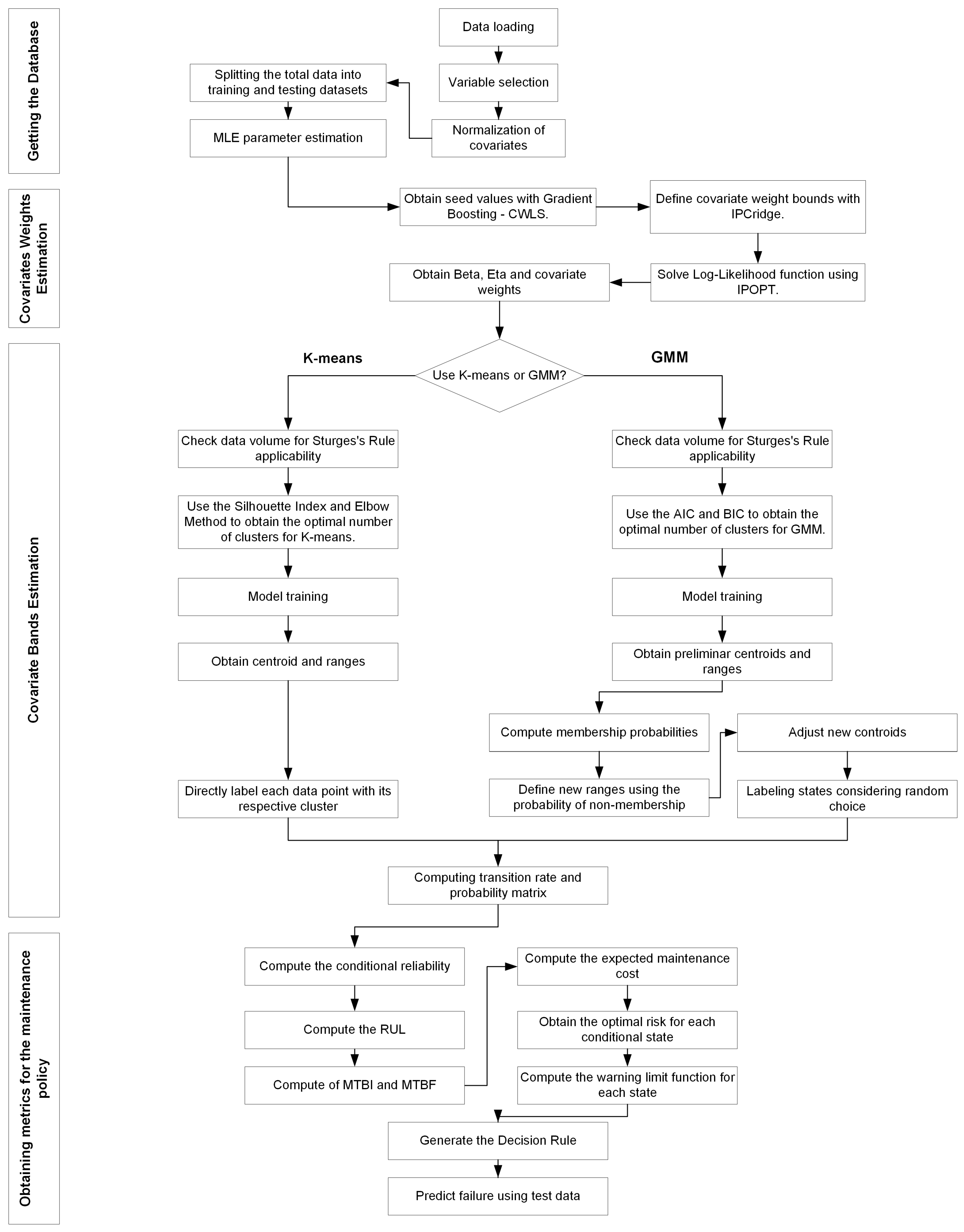
3.5. Proposed Model Structure
Figure 1 illustrates the structure of the proposed model, which is designed to generate a predictive maintenance policy. This model encompasses four key processes: data selection, covariate weight estimation, covariate band estimation, and reliability metrics derivation.

Figure 1.
Structure of the proposed model to define a PHM decision rule from the selection of covariates.
In the data selection phase, data are loaded through a user interface, enhancing the model’s versatility across different databases. Next, covariates are selected and scaled using the NS transformation. Then, the data are split into training and test sets, and preliminary Weibull parameters are estimated.
In the covariate weight estimation phase, the covariate weight estimation process is employed to determine the covariate weights for the proposed PHM-ML model. Initially, gradient boosting with CWLS is used to establish a preliminary weight solution, and IPCRidge is utilized to define variable bounds for the optimization process. Subsequently, IPOPT is applied to minimize the log-likelihood function in Equation (4), thereby obtaining the Weibull parameters and covariate weights for the model.
In the covariate band estimation phase, the band estimation process defines the operational state ranges in the proposed PHM-ML model. Depending on the clustering algorithm, a different process is applied, as detailed in Section 3.3.2. In summary, both algorithms must first determine if class intervals are necessary for data segmentation. Then, the optimal cluster number is identified using the index specific to each clustering technique. For K-means, the ranges and centroids are obtained, directly representing the operational state conditions of an asset. In the case of GMM, an additional process involving the membership probability distribution is applied to define the new ranges and centroids. Finally, the transition rate and probability matrix are computed for both clustering algorithms.
As previously mentioned, the key advantage of these estimation processes is their ability to derive covariate weights and define operational state bands in datasets where expert criteria are unavailable due to insufficient information and the complexity of covariate combinations.
In the final phase, reliability metrics such as conditional reliability, RUL, MTBI, and MTBF are computed to determine the maintenance cost. The optimal risk can be assessed by identifying the optimal time that minimizes this cost. Using this information, the warning limit function is calculated to develop the decision rule that defines the final predictive maintenance policy.
4. Case Study and Results Discussion
The primary aim of this case study is to compare the state band estimation process using K-means and GMM within a real-world operational database. Building upon the research laid by [3], which makes a similar comparison in a synthetic dataset, the present case study takes this a step further in exploring the state band estimation process and how it can lead to the development of decision rules for predictive maintenance policy when dealing with an operational dataset from a Chilean energy distribution company.
To rigorously evaluate the performance of both algorithms and discern potential differences, two distinct models are formulated. The first model leverages the covariate weights and Weibull parameters supplied by the energy company. In contrast, the second model uses the covariate weight process to estimate these parameters.
4.1. Pre-Model Preparation
The dataset encompasses operational and maintenance records from 17 transformers, totaling 93 data points spanning from May 2014 to June 2017. Additionally, the original dataset includes information on 15 vital signals. However, for the purposes of this research, only six covariates are considered. These covariates have been identified as the most pertinent to the condition of the transformers, based on the expert judgment of the company’s maintenance manager. Details of these covariates can be found in Table 1.

Table 1.
Representation of the dataset.
The columns of the dataset are structured as follows. The column is represented in hours since 1 January 1985. The column indicates the operating time in hours since the transformer’s installation. The column denotes the type of intervention performed on the transformer, with 1 indicating preventive and 0 indicating corrective interventions. The column serves as the transformer identifier. Additional columns present covariates considered in the PHM: for electrical demand in megavolt-ampere (MVA), for internal temperature in degrees Celsius (°C), for the temperature difference between internal and ambient readings in degrees Celsius (°C), indicating the ethylene gas percentage in the transformer oil, for the dielectric strength of the transformer oil in kilovolts (kV), and for humidity percentage inside the transformer.
Regarding covariate selection for both models, expert criteria have highlighted the significance of certain variables in modeling the conditional operation of transformers. Specifically, and have been identified as primary determinants, while and are considered secondary covariates of importance. Consequently, the initial model currently employed within the company integrates these four covariates. To evaluate performance relative to this first selection, the second model integrates additional covariates, namely, and , alongside the primary covariates and .
For both models examined in this study, the training dataset consists of approximately 65% of the total data, with the testing dataset comprising the remaining 35%. The study’s time horizon is set at 100,000 h, divided into 500 h intervals. A precision level () of 100 h is chosen for the conditional reliability calculations to optimize computational efficiency. Additionally, a preventive-to-corrective cost ratio of 1:7 is applied for the analysis.
4.2. Model 1: Chilean Company’s Covariate Weights
The initial model integrates covariate weights provided by the Chilean energy company, considered the optimal covariate selection by the expert criteria, which are depicted in Table 2. These weights were computed using the solver and the NS transformation as the scaler.
Table 2.
Covariate weights and Weibull parameters obtained by fmincon and NS scaler for Model 1.
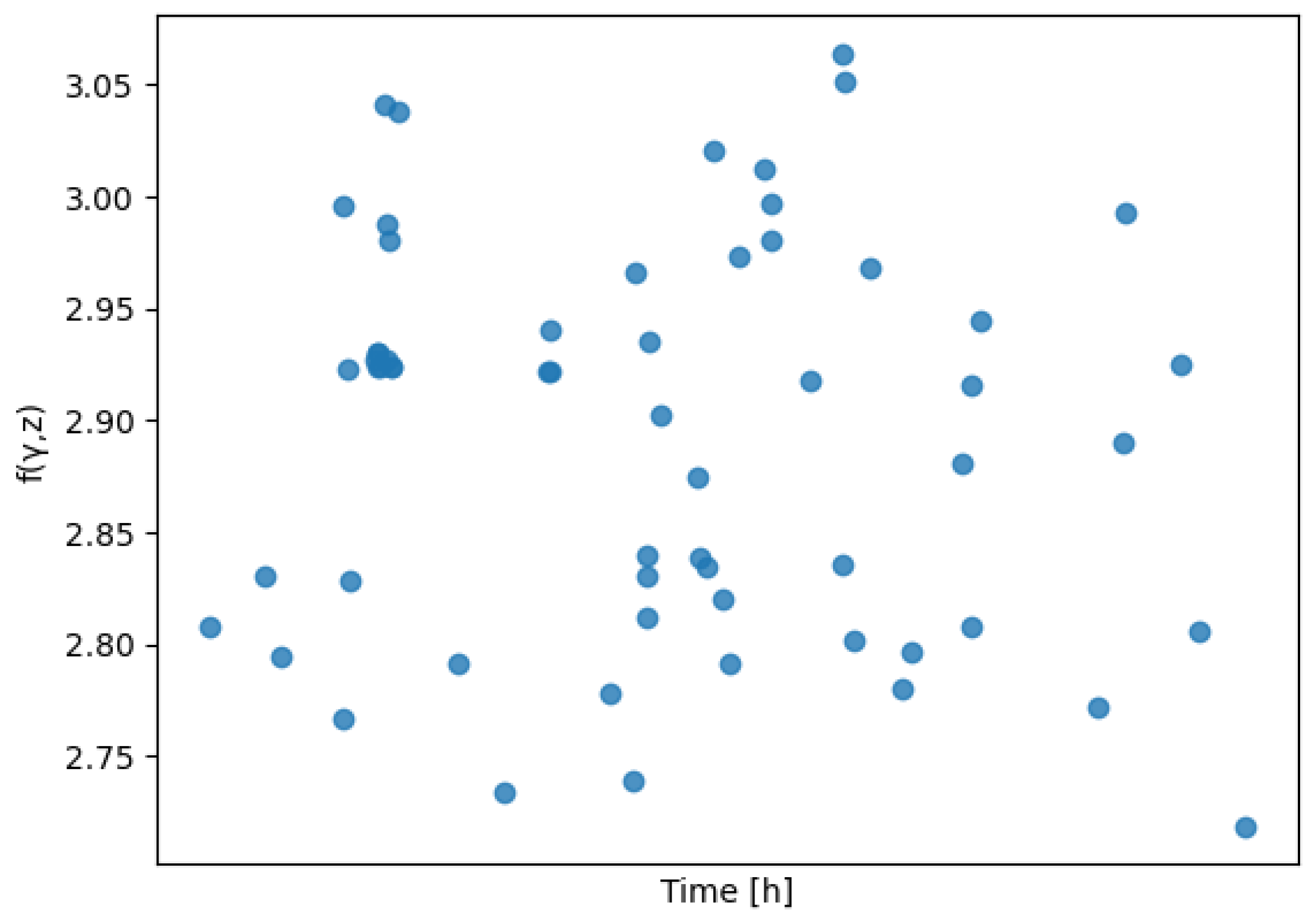
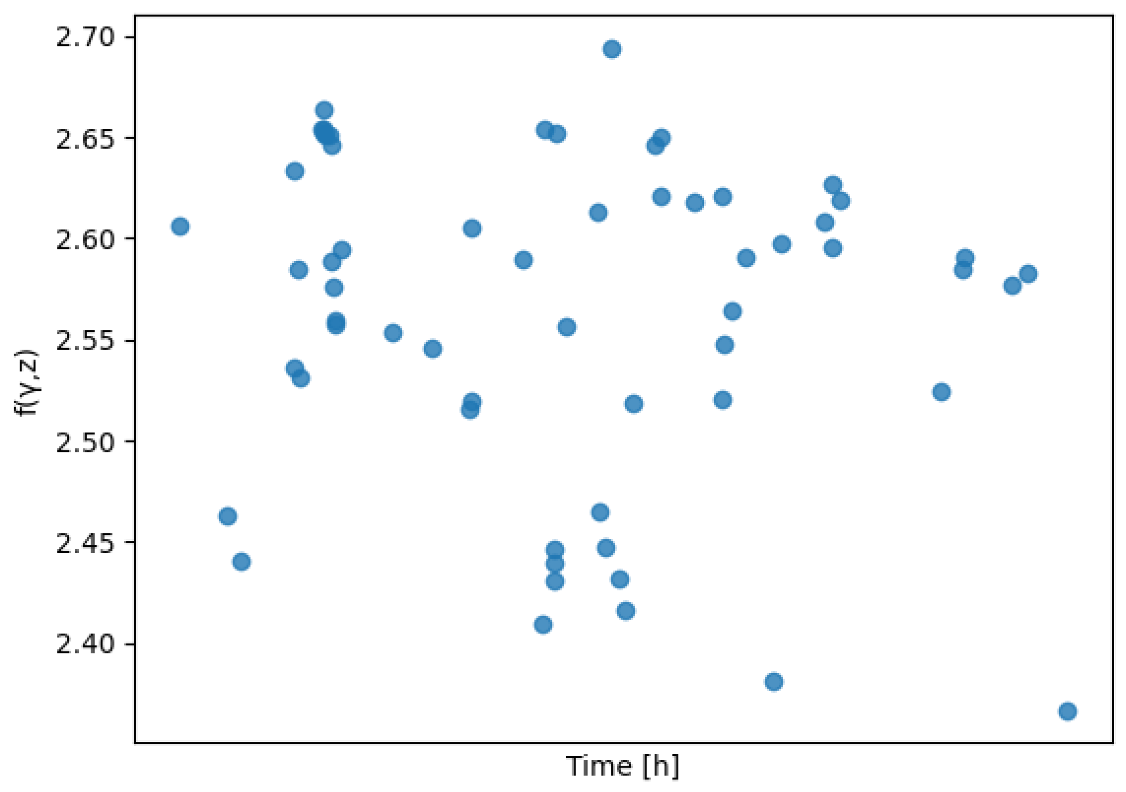
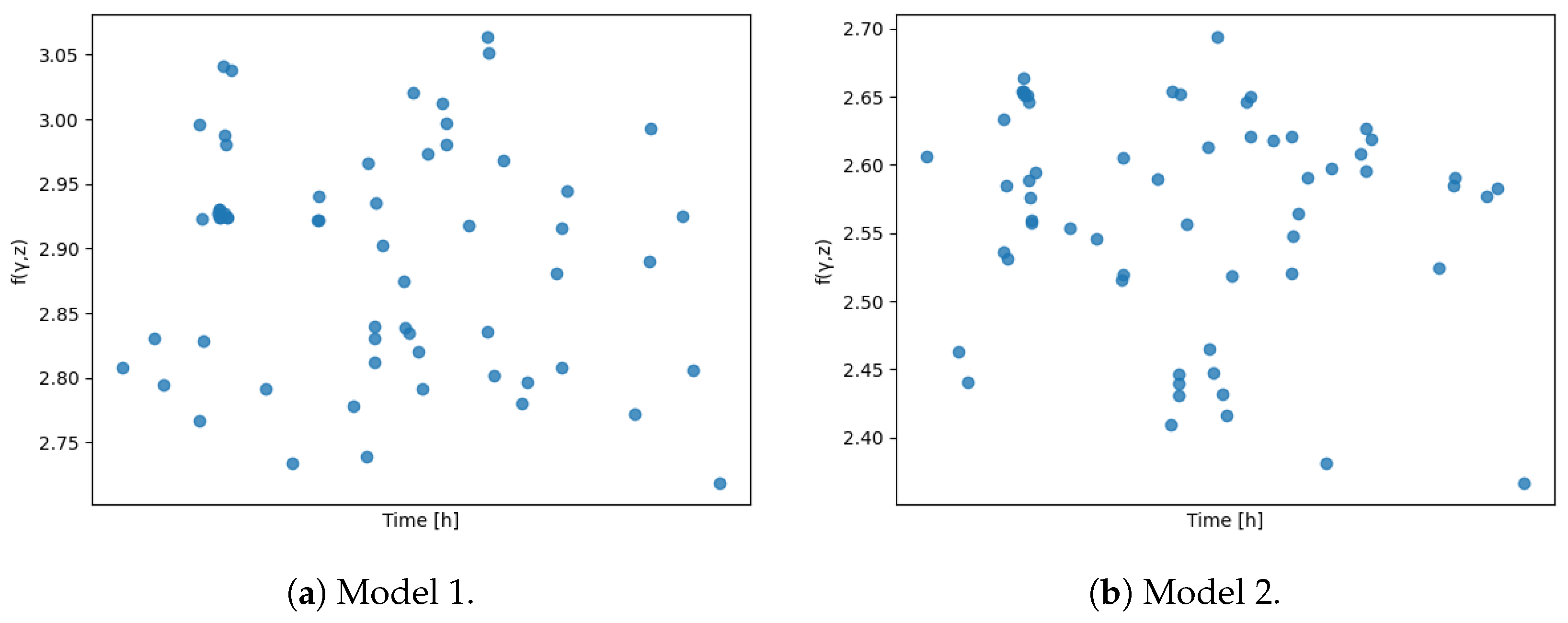
As result of these weights, the composite is computed and shown in Figure 2.
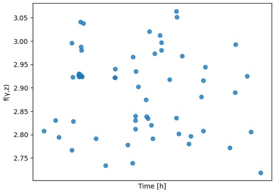
Figure 2.
using the covariate weights from Table 2.
4.2.1. Covariate Weights and Clustering
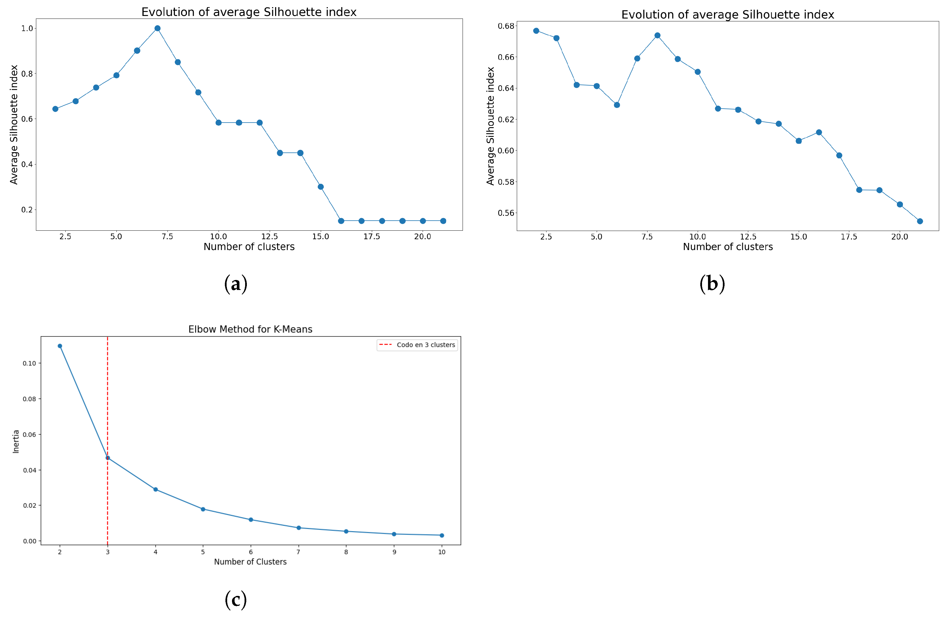
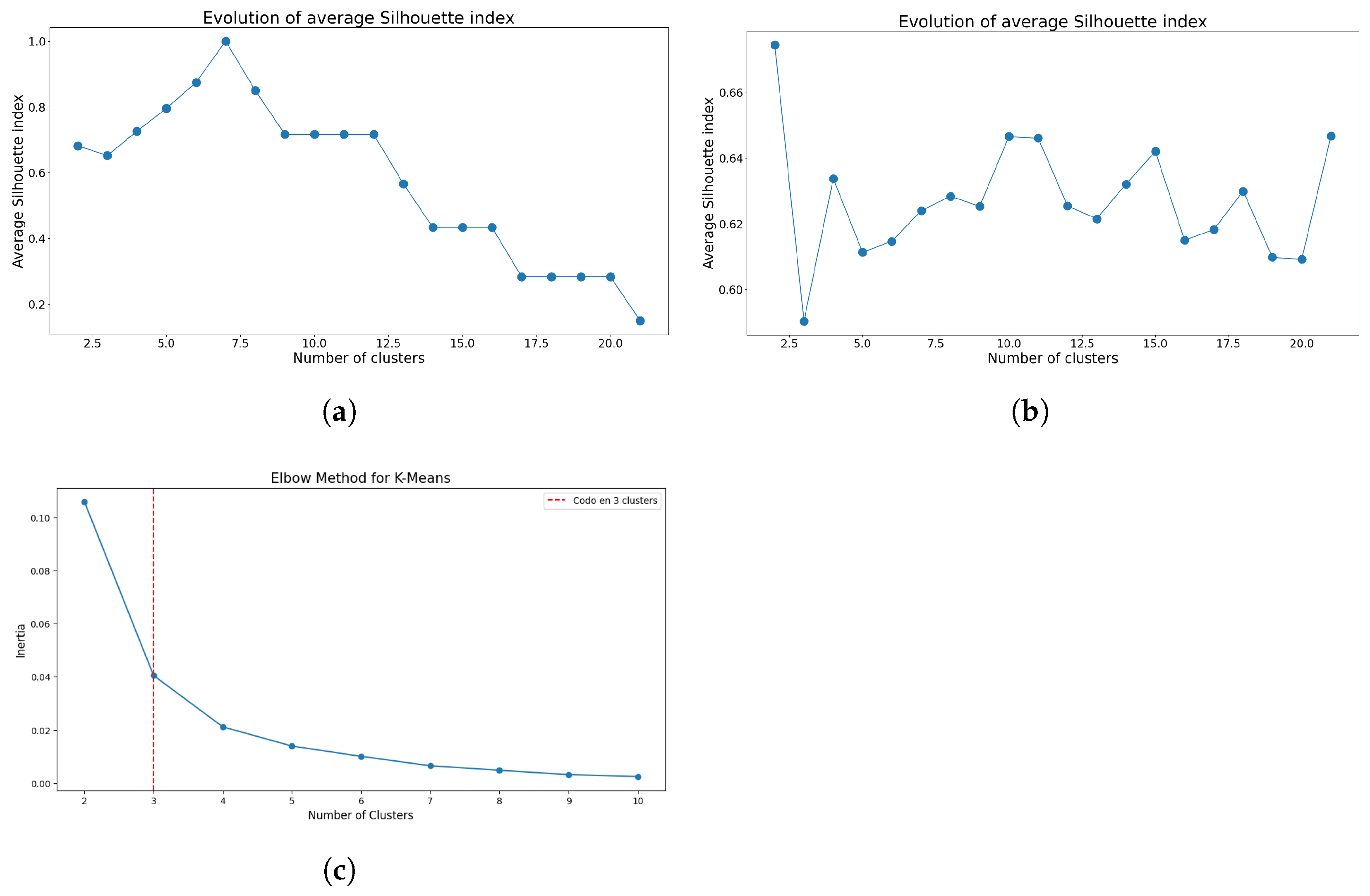
The preliminary analysis focused on determining the optimal number of clusters for both K-means and GMM. Figure 3 and Figure 4 present the respective index results used to ascertain the optimal cluster numbers.
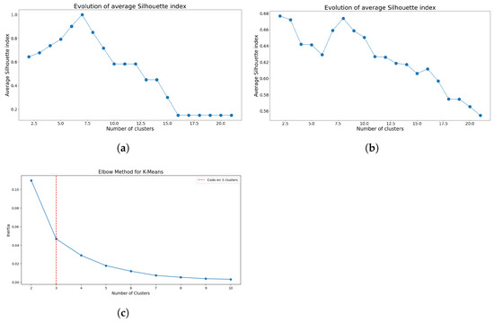
Figure 3.
Indices used to determine the optimal number of clusters using K-means for Model 1. (a) Evolution of silhouette index means using Sturges’ class interval method. (b) Evolution of silhouette index means considering all the data points. (c) Elbow method using inertia index considering all the data points.
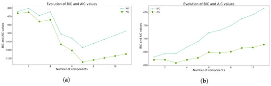
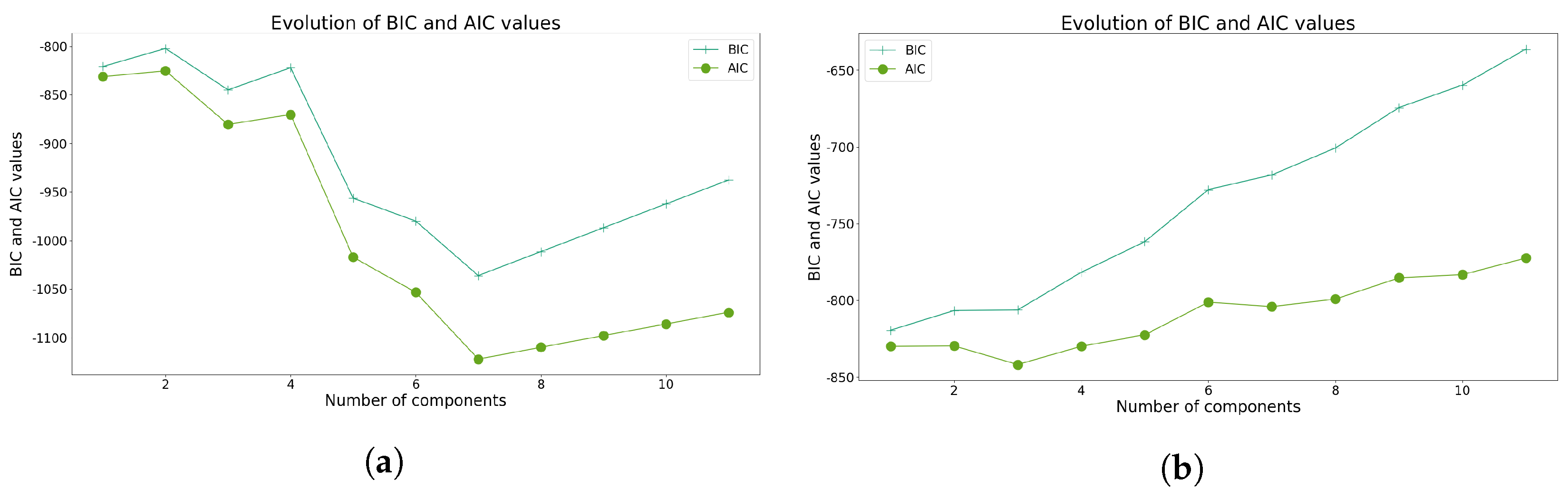
Figure 4.
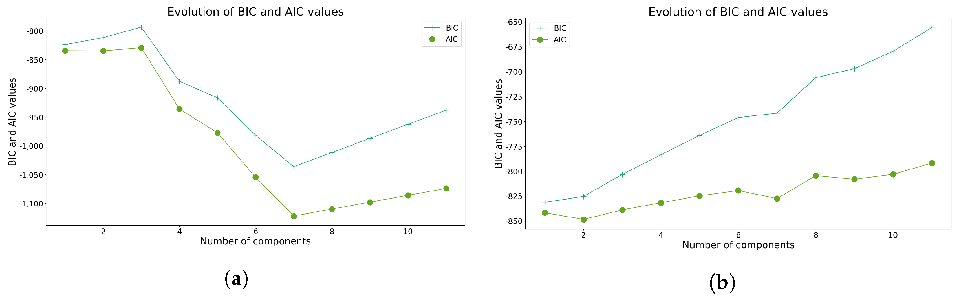
Indices used to determine the optimal number of clusters using GMM for Model 1. (a) Evolution of BIC and AIC scores using Sturges’ class interval method. (b) Evolution of BIC and AIC scores considering all the data points.
The initial findings suggest that class intervals can introduce biases when identifying the optimal number of clusters. Specifically, for K-means, Figure 3a suggests the use of seven clusters, aligning with the number of class intervals generated for the dataset. However, when assessing the silhouette index evolution without applying Sturges’s rule, as illustrated in Figure 3b, that bias disappears, but now the optimal cluster number becomes less definitive and relies on more subjective decision criteria. Nonetheless, employing the elbow method, both with and without class intervals, consistently identifies three as the optimal number of clusters, as depicted in Figure 3c.
In the case of GMM, utilizing class intervals produces results analogous to those obtained without class intervals, as illustrated in Figure 4a, suggesting the adoption of seven clusters. However, employing subjective criteria could justify the selection of three clusters. In contrast, in the absence of class intervals, the optimal AIC value is achieved when opting for three clusters, as evidenced in Figure 4b.
As evidenced, both methodologies encounter difficulties when Sturges’s rule is employed, validating the inherent bias introduced by limited data. Upon eliminating this rule, GMM exhibits enhanced robustness without necessitating an additional index. Nevertheless, three clusters were selected for both models.
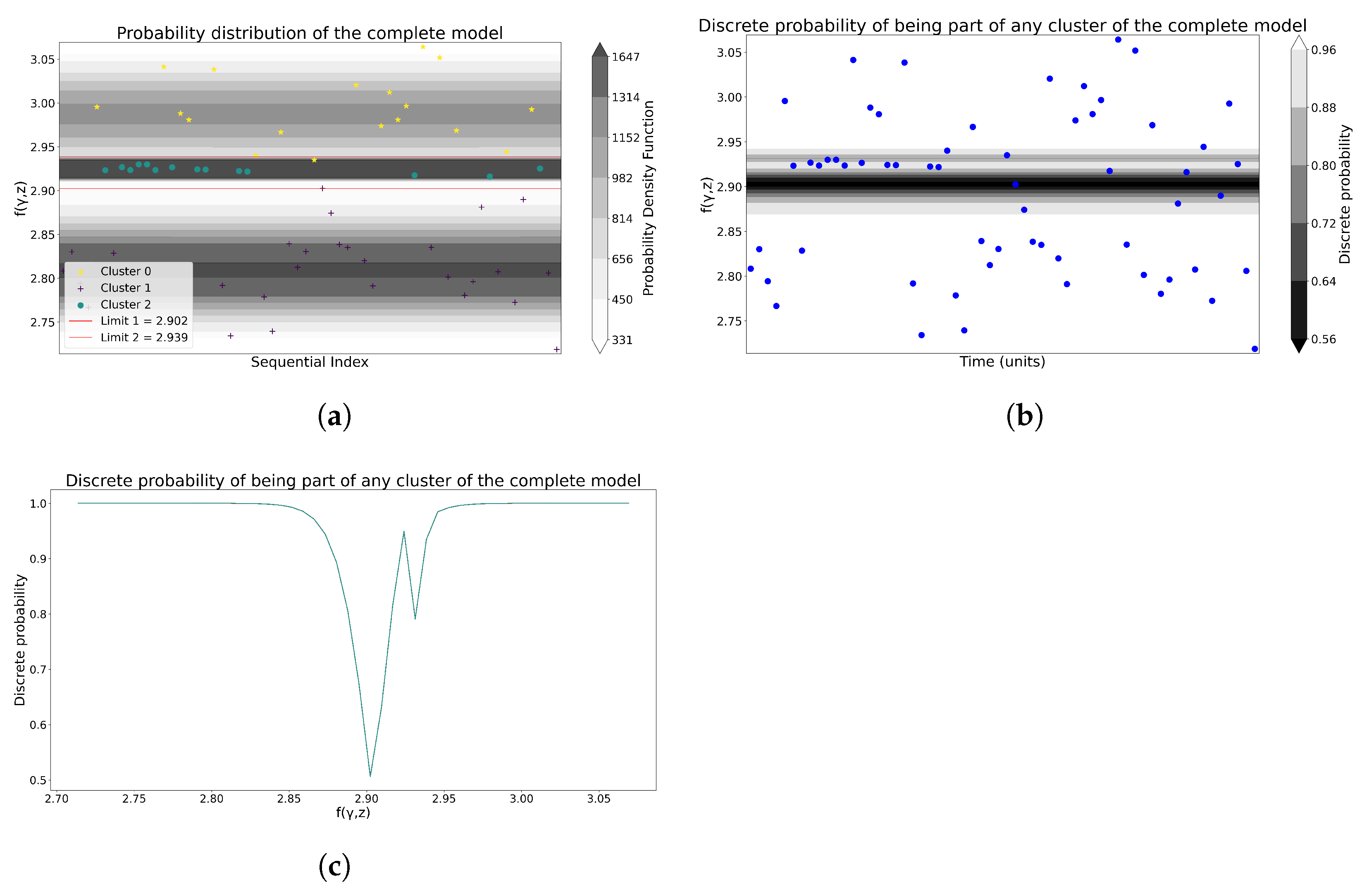
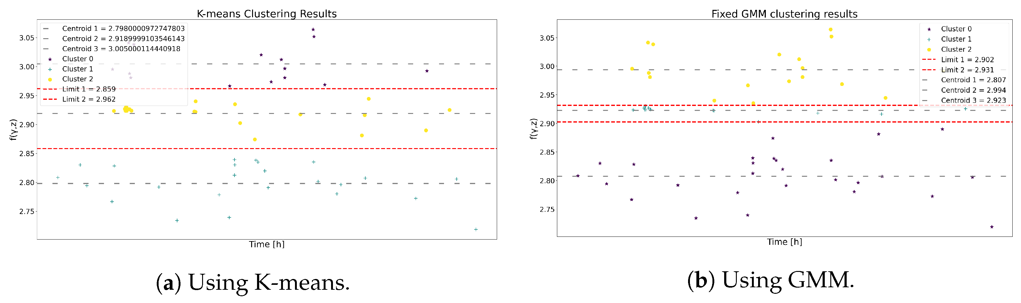
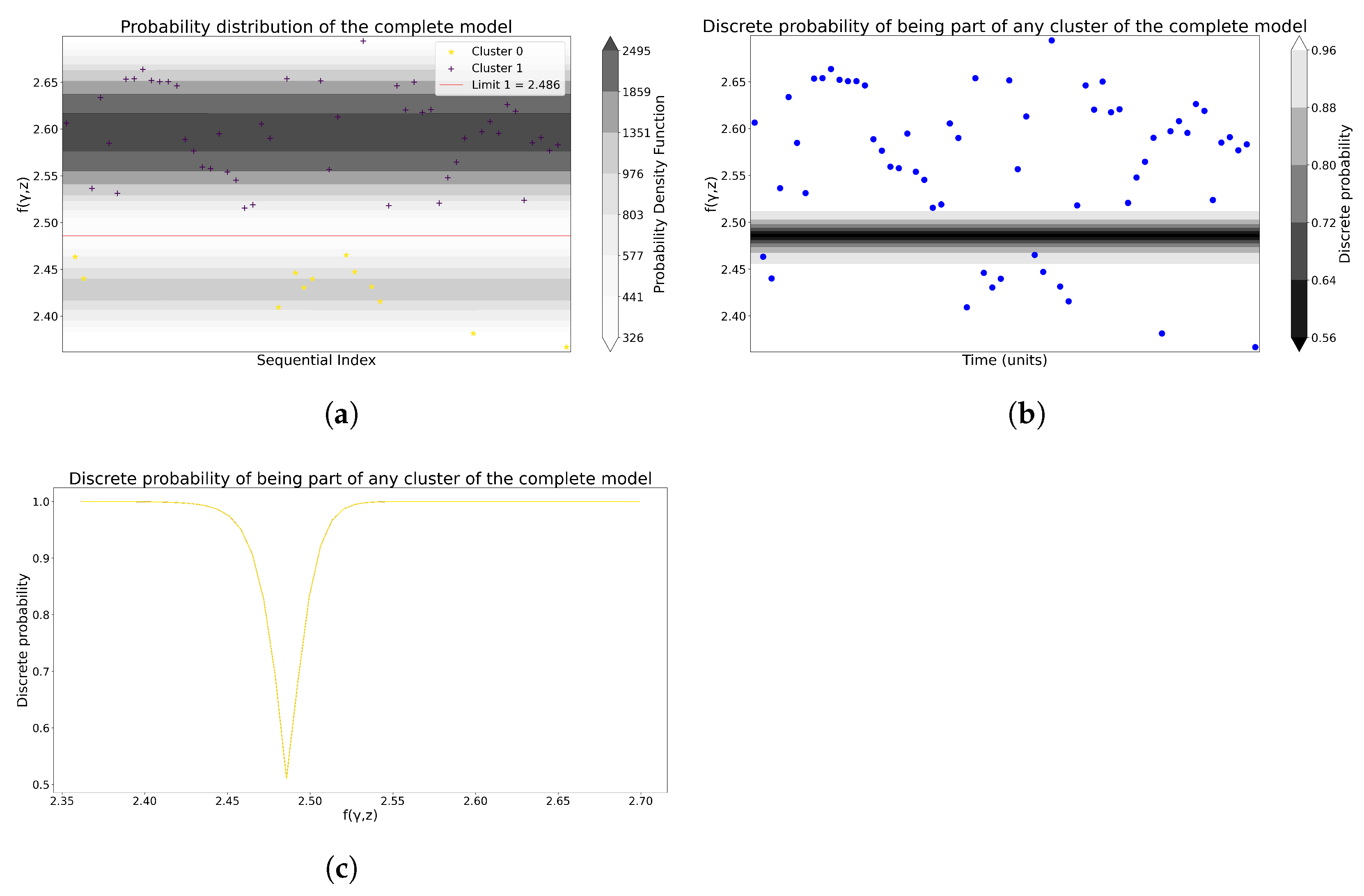
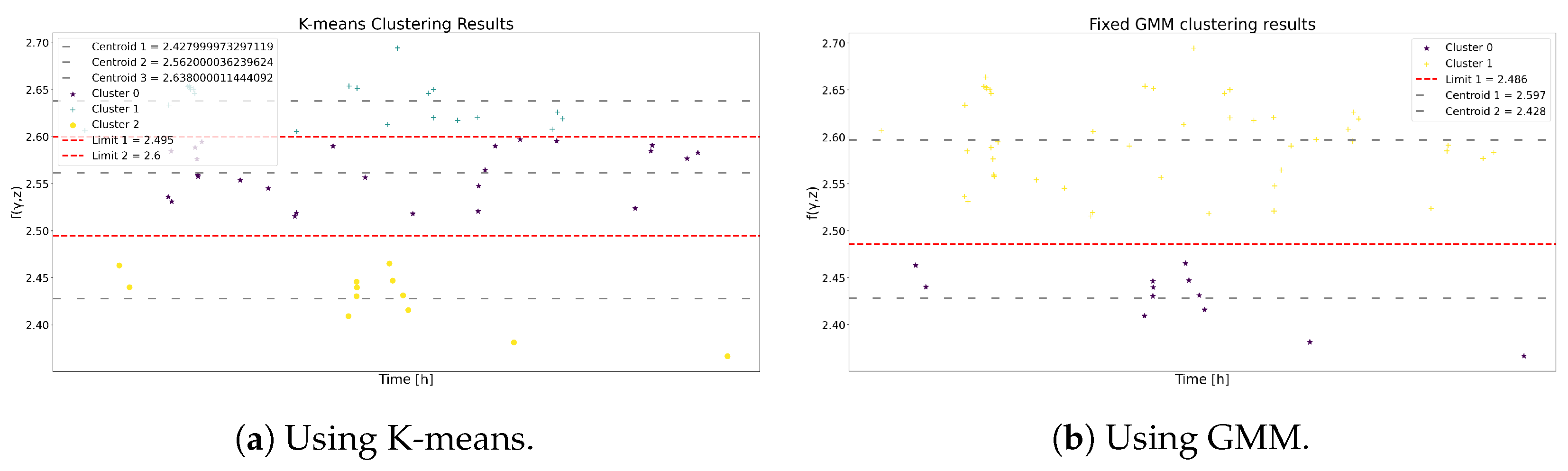
In the case of the GMM, the process in Section 3.3.2 is followed to generate the probability of membership in Figure 5a, as well as the discrete probability of non-membership in Figure 5b,c. Then, Figure 6a and Figure 6b display the cluster boundaries and centroids produced by K-means and GMM, respectively.
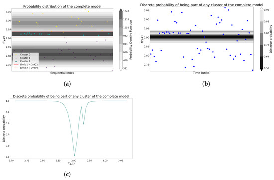
Figure 5.
Joint and discrete probabilities provided by GMM for Model 1. (a) The probability distribution of the entire GMM model. (b) The discrete probability of a GMM being part of any cluster. (c) The discrete probability, from a different perspective, of a GMM being a part of any cluster.
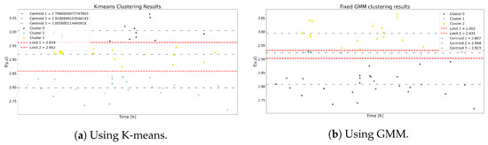
Figure 6.
The clustering results using K-means and GMM for Model 1.
Table 3 and Table 4 show the centroids and the ranges of each state for K-means and GMM. Although the boundary ranges differ, the centroids demonstrate notable similarity. As a result, this resemblance yields comparable outcomes in the state transition probabilities matrix for both methodologies, as depicted in Table 5 and Table 6. Consequently, it is anticipated that the ensuing metrics yield analogous results.
Table 3.
State band limits for each state using K-means for Model 1.
Table 4.
State band limits for each state using GMM for Model 1.
Table 5.
Probability transition matrix using K-means for Model 1.
Table 6.
Probability transition matrix using GMM for Model 1.
4.2.2. Reliability Metrics
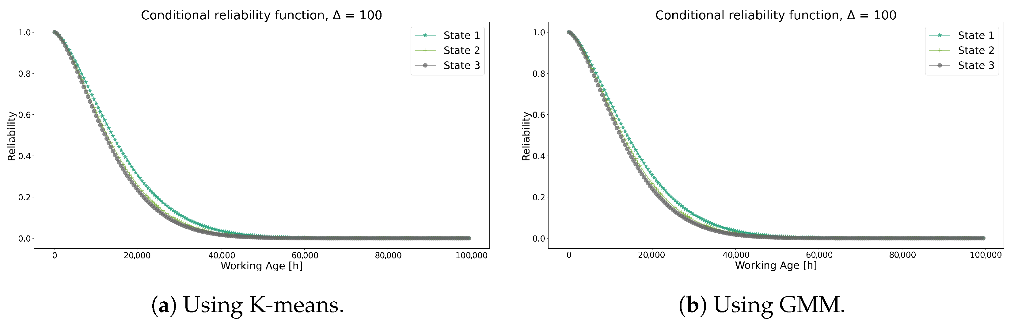
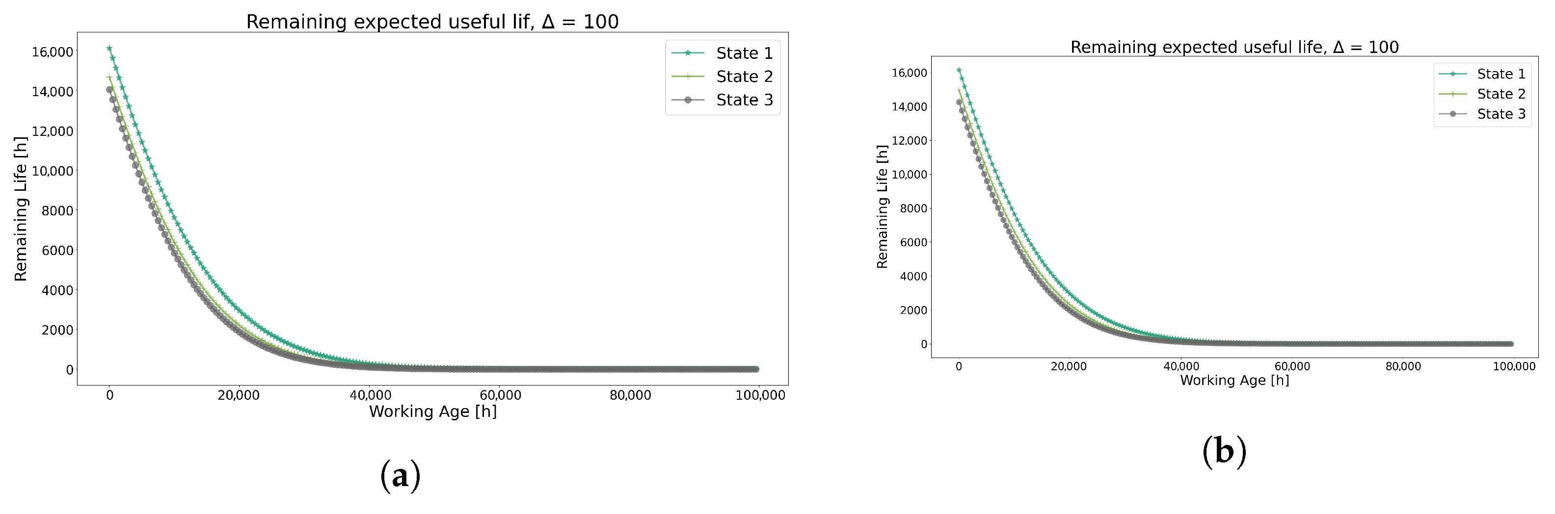
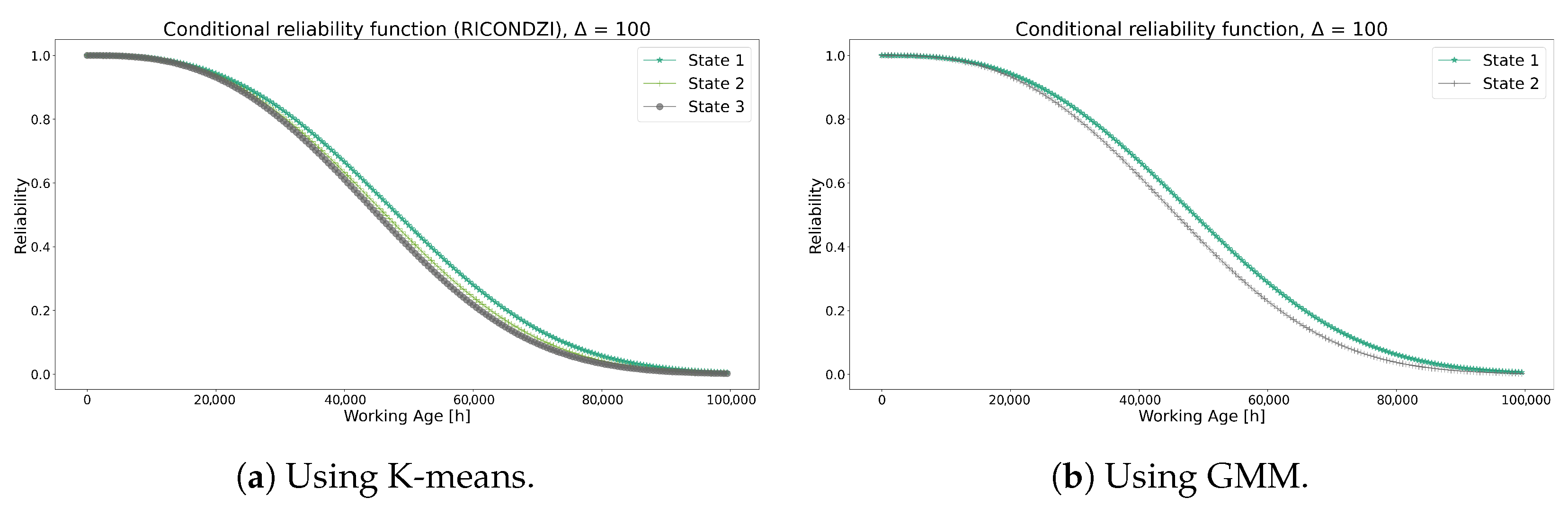
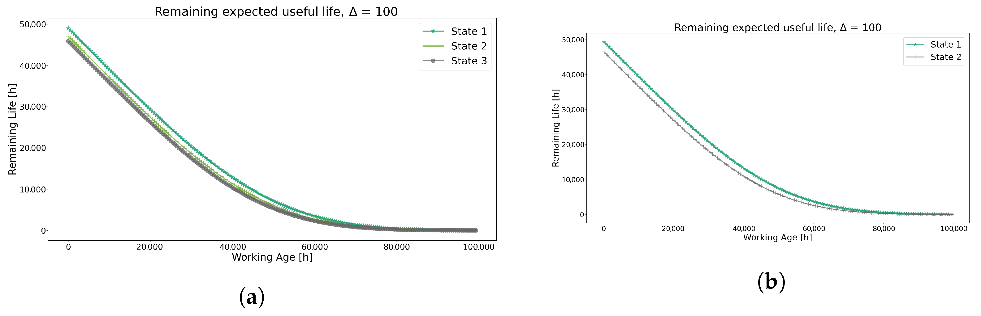
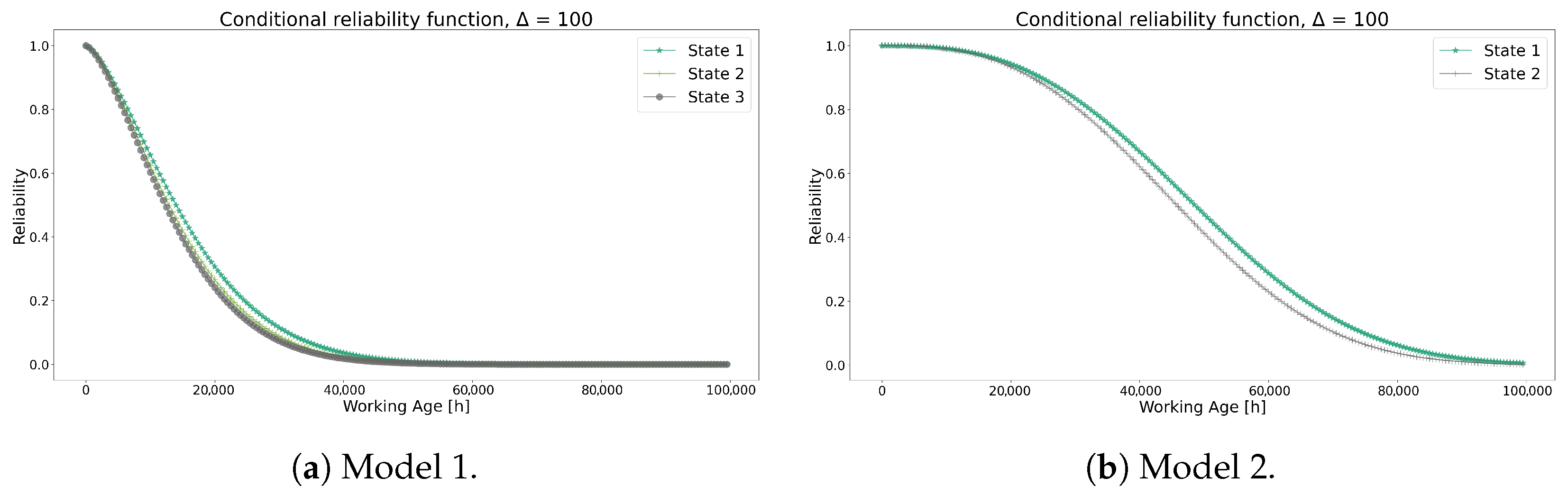
Figure 7 shows the conditional reliability obtained from the K-means and GMM methods where state 1 indicates the most favorable condition from the transformers, and state 3 indicates the least favorable. Comparing both methods results in comparable conditional reliability curves, showing a minor difference between states 3 and 2. While it was expected that the ranges of each state would impact this curve significantly, the transition probability matrices in Table 5 and Table 6 are remarkably similar, as well as the centroids from both algorithms, suggesting the influences of these parameters on the dispersion of each curve state.
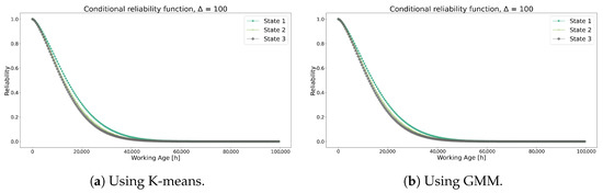
Figure 7.
Conditional reliability functions using each method for Model 1.
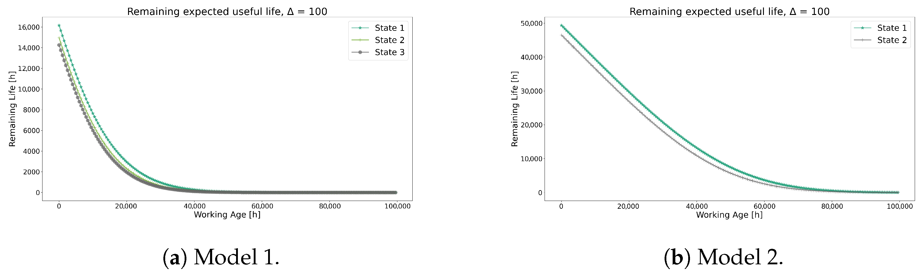
Similar behaviors are observed on the RUL values in Figure 8 for both methods, showing similar curve state dispersion as found in the conditional reliability. These trends are also shown in the MTBI and MTBF values.
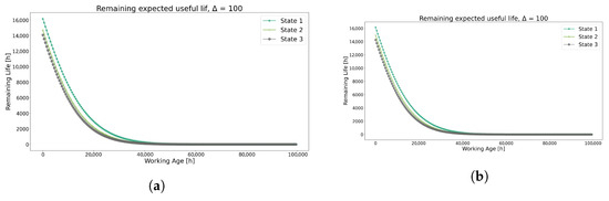
Figure 8.
Prediction of RUL using each method for Model 1. (a) Remaining Useful Life prediction using the K-means method. (b) Remaining Useful Life prediction using the GMM method.
The analysis of the optimal time obtained through the cost function reveals comparable outcomes for both algorithms, as demonstrated in Table 7, which exhibit identical optimal times and show a close similarity between each state time.
Table 7.
Optimal time considering the cost function results using each method for Model 1.
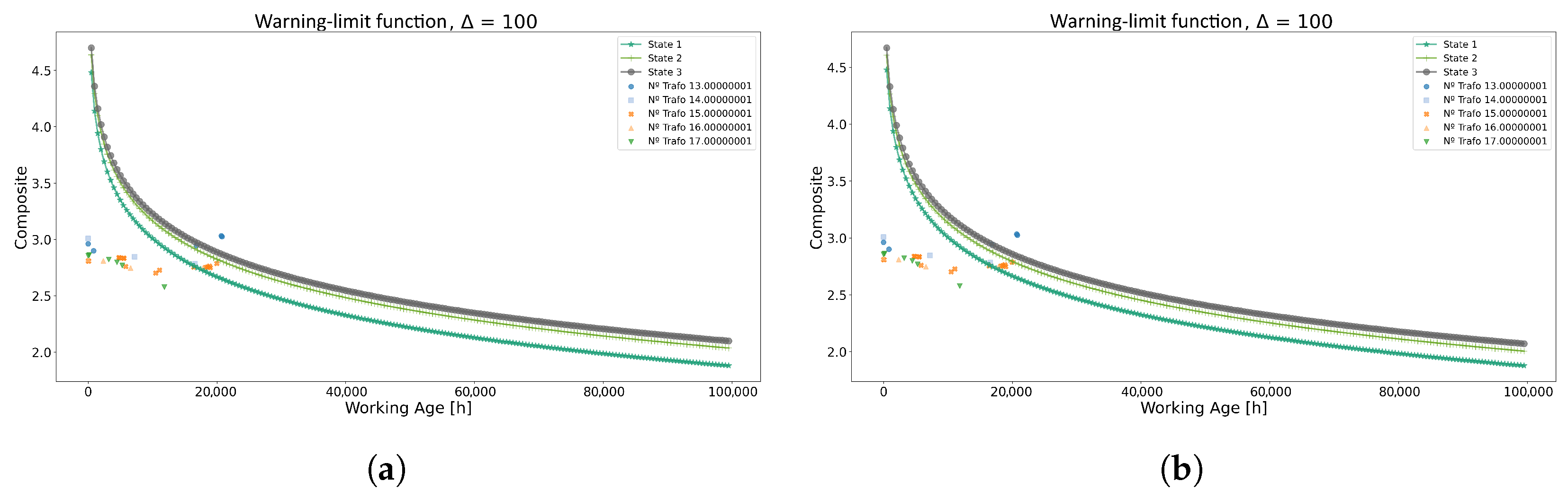
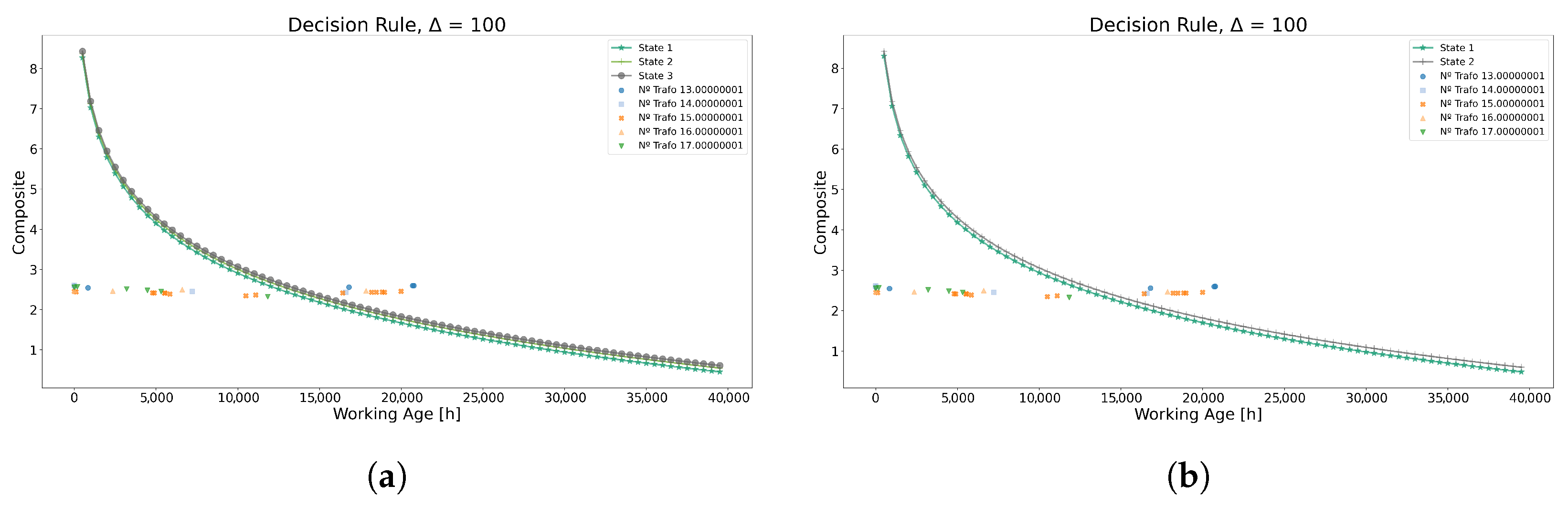
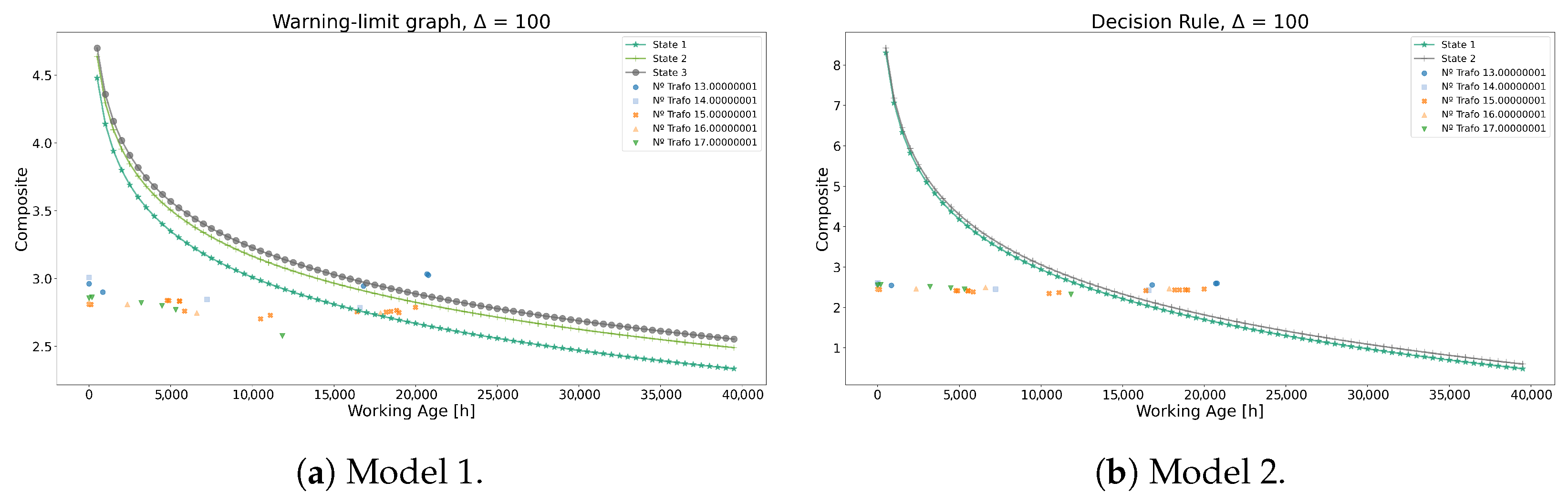
Based on these findings, the maintenance policies derived from both methodologies exhibit striking similarities, as illustrated in Figure 9. Moreover, data points from the test dataset are overlaid above the decision policy graph: data points representing normal operations fall below the curve of state 1. Conversely, data points situated between states 1 and 3 indicate a need for caution and preparation for replacement, while those above the curve of state 3 signify an imminent risk of failure, necessitating immediate intervention.
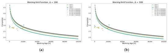
Figure 9.
Warning limit function using each method for Model 1. (a) Warning-limit function using the K-means method. (b) Warning-limit function using the GMM method.
As observed in Figure 9, both graphs indicate that power transformer 13 requires immediate intervention at the 20,000 h mark. Conversely, power transformers 14 and 15 are situated in the caution zone at the 18,000 h and 20,000 h marks, respectively, suggesting a need for replacement in the near future. As for the remaining transformers, no intervention is necessary as they are operating within acceptable parameters.
Finally, the policies formulated from both approaches were compared with the maintenance policy employed internally by the Chilean company, revealing nearly identical intervention decisions.
4.2.3. Results Discussion
Based on the findings of this first analysis, several takeaways emerged:
Initially, it is demonstrated that the quantity of available data plays a pivotal role in determining the optimal number of clusters. In the context of K-means clustering, the incorporation of additional indices was found to be essential to avoid subjectivity in cluster determination. In contrast, GMM demonstrated a higher degree of robustness by solely relying on AIC and BIC scores for identifying the objective optimal number of clusters. Consequently, the GMM emerges as a preferable approach for minimizing potential biases inherent in the data.
Secondly, despite the differences in state ranges produced by the two algorithms, the reliability metrics generated were remarkably consistent and similar. This result can be explained by the parallelism observed in the probability transition matrix, which was largely led by the centroid values of each model. Although these findings are not expected, they may be influenced by the selected covariates and weights of this model. Consequently, in the following analysis, the second model is used to assess whether the selection of covariates significantly impacts the performance of the resultant policy.
Finally, the collection of the warning limit function can facilitate the development of a decision rule to intervene with the power transformers and formulate a predictive maintenance policy, thereby achieving the established goal of this study.
4.3. Model 2: Self-Generated Covariate Weights
In the second model, as stated in the pre-model preparation section, a different combination of significant covariates and less significant ones is employed to assess whether different performance in reliability metrics can be achieved. Specifically, the covariates , , , and are used. Additionally, the optimization parameters utilized include the IPOPT optimization with the NS scaler and IPCRidge, resulting in the covariate weights presented in Table 8.
Table 8.
Covariate weights and Weibull parameters obtained by fmincon and NS scaler for Model 2.
Based on these weights, the composite is calculated and displayed in Figure 10. This composition exhibits a distinct structure compared to the one derived from the previous model, as illustrated in Figure 2.
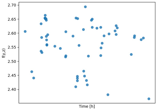
Figure 10.
using the covariate weights from Table 8.
4.3.1. Covariate Weights and Clustering
Consistent with the previous analysis, the primary focus is on identifying the optimal number of clusters for both K-means and GMM. Figure 11 and Figure 12 show the respective index results utilized to determine the optimal cluster configurations.
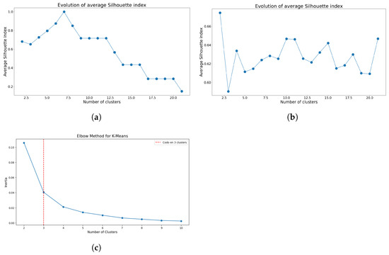
Figure 11.
Indices used to determine the optimal number of clusters using K-means for Model 2. (a) Evolution of silhouette index means using Sturges’ class interval method. (b) Evolution of silhouette index means considering all the data points. (c) Elbow method using inertia index considering all the data points.
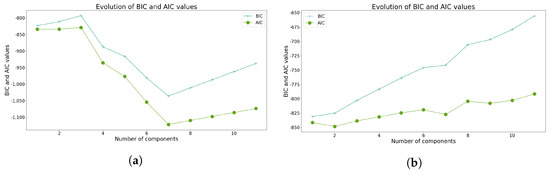
Figure 12.
Indices used to determine the optimal number of clusters using GMM. for Model 2. (a) Evolution of BIC and AIC scores using Sturges’ class interval method. (b) Evolution of BIC and AIC scores considering all the data points.
The trend related to the bias introduced by class intervals remains consistent. For K-means, Figure 11a suggests seven clusters, aligning with the number of class intervals. Without applying Sturges’s rule, Figure 11b presents a less definitive optimal cluster number. As anticipated, the elbow method consistently identifies three clusters as optimal, as illustrated in Figure 11c.
In the case of the GMM, the use of class intervals reintroduces the previously observed bias, as illustrated in Figure 12a, suggesting the adoption of seven clusters. However, subjective criteria could justify opting for two clusters. In contrast, without class intervals, the optimal AIC value is achieved with two clusters, as shown in Figure 12b. Furthermore, these results differ from those of the previous model, indicating that changes in covariates can lead to varying outcomes.
For GMM, the distribution probabilities are shown in Figure 13. Figure 14a,b display the cluster boundaries and centroids generated by K-means and GMM, respectively.
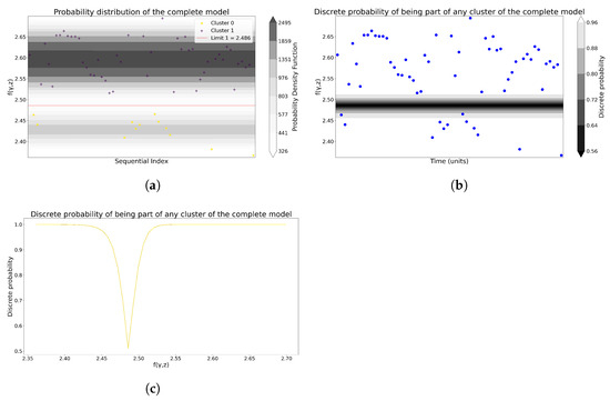
Figure 13.
Joint and discrete probabilities provided by the GMM model for Model 2. (a) The probability distribution of the entire GMM model. (b) The discrete probability of a GMM being part of any cluster. (c) The discrete probability, from a different perspective, of a GMM being a part of any cluster.
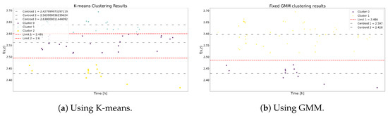
Figure 14.
The clustering results using K-means and GMM for Model 2.
Table 9 and Table 10 demonstrate that, despite differences in state and band ranges, the magnitudes of the centroids are closely aligned. This discrepancy has a negligible impact on the transition probabilities matrix for both methodologies, as shown in Table 11 and Table 12. Therefore, it is anticipated that the subsequent metrics produce similar results.
Table 9.
State band limits for each state using K-means for Model 2.
Table 10.
State band limits for each state using GMM for Model 2.
Table 11.
Probability transition matrix using K-means for Model 2.
Table 12.
Probability transition matrix using GMM for Model 2.
4.3.2. Reliability Metrics
Figure 15 illustrates comparable behavior between the two clustering methods, with the exception that GMM has fewer conditional states than K-means. Similar trends are observed in the RUL values depicted in Figure 16 for both methods.
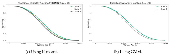
Figure 15.
Conditional reliability functions using each method for Model 2.
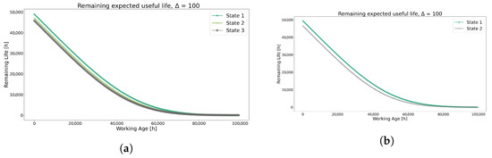
Figure 16.
Prediction of RUL using each method for Model 2. (a) Remaining Useful Life prediction using the K-means method. (b) Remaining Useful Life prediction using the GMM method.
The analysis of optimal times reveals that the instances where costs are minimized are clustered closely together for both clustering techniques, as evidenced in Table 13.
Table 13.
Optimal time considering the cost function results using each method for Model 2.
These findings confirm that maintenance policies derived from both methodologies share significant similarities, as illustrated in Figure 17. Regarding the intervention policy, both decision rules suggest that the power transformers numbered 13, 14, 15, and 16 should have been subject to an intervention at the 15,000 h mark as they are located in the warning zone. Meanwhile, only transformer 17 is located in the safe zone. However, due to the close dispersion of the conditional states, it is also expected to be subject to an intervention when it surpasses the 15,000 h mark.
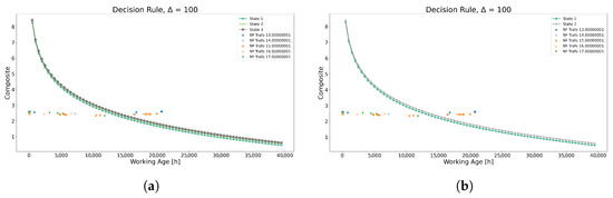
Figure 17.
Warning limit function using each method for Model 2. (a) Warning-limit function using the K-means method. (b) Warning-limit function using the GMM method.
4.3.3. Results Discussion
Based on the findings of this second analysis, several takeaways emerged:
Initially, it is confirmed that the amount of available data significantly impacts the optimal number of clusters. As seen in both models, K-means necessitates additional indices to avoid subjective criteria when determining the optimal cluster count. In contrast, GMM demonstrates greater robustness by relying solely on the AIC and BIC scores. Therefore, careful selection is crucial when choosing between these algorithms. Overall, GMM proves to be the preferred option over K-means in this context.
Secondly, this analysis again reveals that the difference between state bands and centroids has minimal impact on reliability metrics. This second model was essential to understand that this effect was not caused by the centroid values themselves, but rather by the closeness in their magnitudes. This is evident in the examples of K-means and GMM, where the centroid values do not perfectly align.
While both clustering algorithms might suggest minimal difference in application, previous studies have shown that GMM and K-means can yield different results with more data. For this paper, GMM is a more suitable choice due to its use of membership probabilities, which creates more intuitive boundaries.
With the new selection of covariates, the decision rules suggest more aggressive interventions than the first model. Nevertheless, it still demonstrates that the proposed model can assist in defining predictive maintenance policies, with its performance dependent on the conditions alternative.
4.4. Performance Comparison between Both Models
This final section is focused on evaluating the performance of both models by comparing their reliability metrics and final decision rules. Through this analysis, a better understanding of the importance of covariate selection can be obtained, and further insight into the covariate weight and band estimation process can also be gained. Consequently, both models applied in the previous analyses are compared using the GMM clustering technique.
Table 14 shows the covariate weights obtained from both models. The first noticeable difference is the significant variance in the values, indicating that selecting the covariates of Model 2 leads to an overall worse deterioration of the power transformers compared to those selected in Model 1. However, while the magnitudes of are similar between the models, it is noteworthy that Model 2 exhibits a slightly larger value than Model 1, compensating slightly for the high degradation rate it exhibits. Regarding the covariate weights, both models exhibit similar magnitudes for the covariates and . Furthermore, the covariate emerges as the most significant covariate with the highest weight values, partly confirming expert judgment regarding the high significance of these covariates.
Table 14.
Weibull parameters and covariate weights for Model 1 and Model 2.
4.4.1. Covariate Weights and Clustering
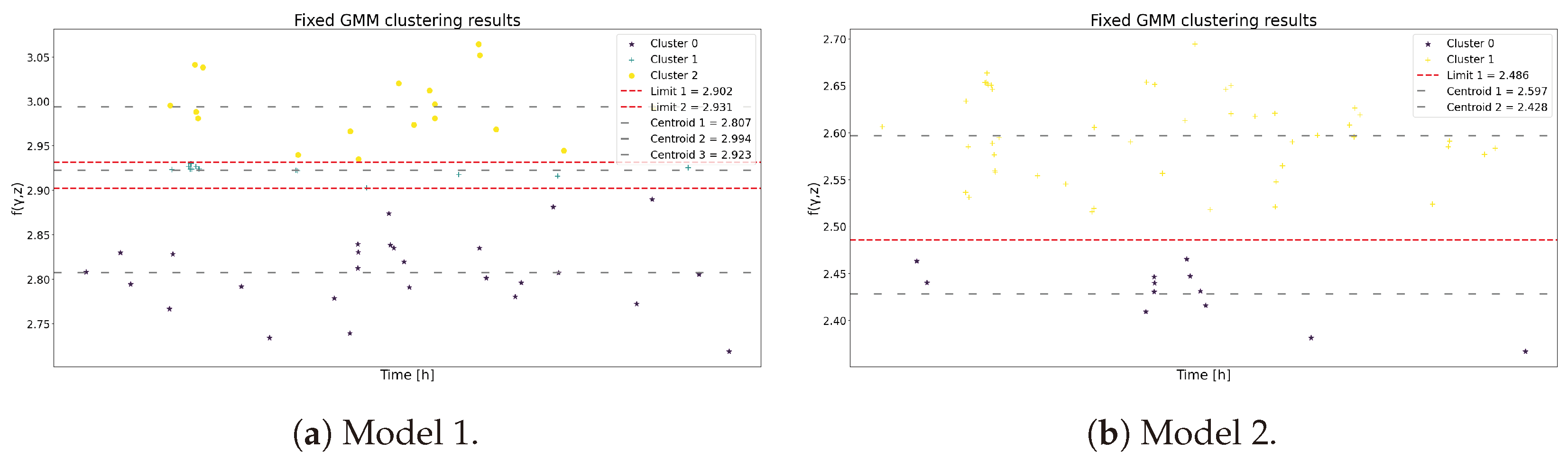
As shown in the previous analysis, the composite of both models can be compared in Figure 18. It is evident that the selection of different covariates results in distinct data compositions. In Model 1, the data are more evenly distributed, whereas in Model 2, the data tend to accumulate in the upper zone. Notably, Model 2 makes the potential segmentation of the data more visually apparent, which is confirmed in Figure 19. Furthermore, both models exhibit distinct operational states when using GMM as the clustering technique, with Model 2 presenting a smaller cluster. This may indicate that Model 2 favors simplicity compared to the original model based on expert criteria. However, despite the similar magnitudes of the composites, the results from the previous analyses suggest that the models yield different outcomes. Finally, the probability transition matrices are compared in Table 15.
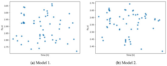
Figure 18.
for Model 1 and Model 2 using the covariate weights from Table 14.
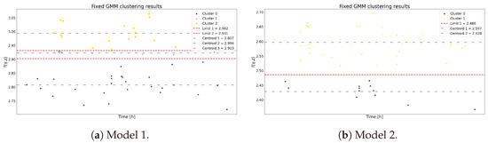
Figure 19.
The clustering results for Model 1 and Model 2 using GMM.
Table 15.
Probability transition matrix for Model 1 and Model 2.
4.4.2. Reliability Metrics
Figure 20 compares the conditional reliability of both models, highlighting noticeable differences. Initially, even though Model 1 exhibits a lower value than Model 2, it produces reliability curves with a greater penalization. As observed in the separate analysis of each model, the combination of values and the transition probabilities in Table 15 likely resulted in the more optimistic reliability curves seen in Model 2. Furthermore, this behavior is also reflected in the RUL values shown in Figure 21.
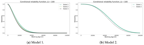
Figure 20.
Conditional reliability functions for Model 1 and Model 2.
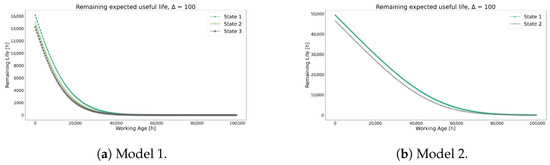
Figure 21.
Prediction of RUL for Model 1 and Model 2.
Continuing the comparison, Table 16 presents the optimal replacement times, revealing a notable contrast between the models. This divergence manifests in distinct warning limit graphs illustrated in Figure 22. Model 2 demonstrates a significantly more aggressive approach compared to Model 1, necessitating earlier interventions for transformers 13, 14, 15, and 16 at the 15,000 h mark, whereas in Model 1, only transformer 13 requires intervention at the 21,000 h mark. Additionally, Model 1’s curves exhibit greater dispersion, offering additional insights into the equipment’s operational states within the caution zone, whereas Model 2’s curves display less dispersion, suggesting diminished information quality and a nearly binary decision-making process. Despite these disparities, Model 2, deemed less optimal according to expert judgment, achieves relatively similar outcomes, serving as a viable alternative when expert recommendations are unavailable.
Table 16.
Optimal time considering the cost function results for Model 1 and Model 2.
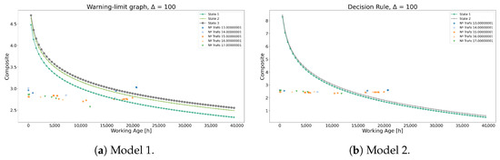
Figure 22.
Decision rules under Model 1 and Model 2.
4.4.3. Results Discussion
Based on the results of this final analysis, several insights have emerged:
The comparison between both models across various reliability metrics highlights the significant impact of selecting different covariates. Even when keeping two covariates fixed, differences in weights are sufficient to generate distinct data compositions, cluster numbers, and reliability metrics. This outcome underscores the importance of developing new strategies for achieving optimal and non-arbitrary covariate selection.
Regarding the results themselves, it was anticipated that the model recommended by expert criteria would outperform a sub-optimal model. However, while Model 2 yields more optimistic conditional reliability than Model 1, it fails to capitalize on this optimism when generating maintenance policies, resulting in a more conservative approach. This discrepancy may be influenced by data composition or state transition probabilities and warrants further investigation in future research.
Finally, it is noteworthy that Model 2 is not entirely distant from Model 1’s performance, and both models generate feasible policies. This result suggests that in cases where expert criteria are not available, the proposed model can produce robust results. Moreover, this finding underscores the capabilities of the covariate weight and band state estimation processes to adapt to multi-condition scenarios without expert knowledge. This adaptability is evident in Model 1, where expert criteria lacked information about covariate values or state band ranges. Thus, this analysis demonstrates that jointly using these processes can provide significant value to the maintenance area in scenarios where such information is absent.
5. Conclusions
This study presents a comprehensive model of clustering techniques to determine the most suitable algorithm for developing advanced predictive maintenance policies in multi-covariate scenarios in industries where real-time data are readily available. Two models were formulated, each featuring distinct covariates and weights. Hence, decision rules for both models are generated to evaluate their predictive intervention performance.
The in-depth analysis revealed the critical role of data quantity in determining the optimal number of clusters for both techniques. Notably, unlike K-means, GMM demonstrated greater robustness, eliminating the need for additional indices and subjective criteria. Moreover, GMM’s cluster segmentation, based on probability distributions, is more interpretable. The study found that the magnitude of data variation has a greater impact than the state band and centroid values, as shown by the significant similarity of the K-means and GMM policies. Furthermore, when comparing both models, while the one suggested by expert criteria yields a reasonable maintenance policy, the latter demonstrates strong performance. Especially in cases where expert knowledge is absent, the proposed model is extremely useful and a vital guide for condition-based maintenance under a predictive approach. This research also highlights the robustness of the covariate weight and band state estimation processes in multi-condition scenarios, suggesting their ability to identify near-optimal solutions regardless of specific covariate selections and their replicability across different datasets.
In summary, this research has identified the best overall clustering algorithm for a multi-covariate industrial scenario. It has demonstrated that the condition weight estimation process can achieve robust results, highlighting the potential value of integrating covariate weight and state band processes. Consequently, further works could prioritize the implementation of these methods and explore novel approaches for selecting optimal covariates. Finally, seamlessly integrating all these processes into a PHM-ML scheme capable of cross-industry applications strengthens the guidance in pursuit of advanced predictive maintenance decisions.
Author Contributions
Conceptualization, D.R.G.; Methodology, D.R.G.; Validation, D.R.G., C.M., R.M., F.K. and P.V.; Formal analysis, D.R.G.; Investigation, D.R.G. and C.M.; Writing—original draft preparation, D.R.G. and C.M.; Writing—review and editing, D.R.G., C.M., R.M., F.K. and P.V.; Supervision, D.R.G.; Project administration and Funding acquisition, D.R.G. All authors have read and agreed to the published version of the manuscript.
Funding
This research was supported by ANID through FONDEF—Concurso IDeA I+D (Chile). Grant Number: ID22I10348.
Data Availability Statement
Data is contained within the article.
Acknowledgments
The authors wish to acknowledge the financial support of this study by Agencia Nacional de Investigación y Desarrollo (ANID) through Fondo de Fomento al Desarrollo Científico y Tecnológico (FONDEF) of the Chilean Government (Project FONDEF IDeA ID22I10348).
Conflicts of Interest
The authors declare no conflict of interest.
References
- Ali, A.; Abdelhadi, A. Condition-Based Monitoring and Maintenance: State of the Art review. Appl. Sci. 2022, 12, 688. [Google Scholar] [CrossRef]
- Jardine, A.K.S.; Group, T.F.; Tsang, A.H.C.; Taghipour, S. Maintenance Replacement and Reliability: Theory and Applications, 3rd ed.; CRC Press: Boca Ratón, FL, USA, 2021. [Google Scholar]
- Godoy, D.R.; Álvarez, V.; López-Campos, M. Optimizing Predictive Maintenance Decisions: Use of Non-Arbitrary Multi-Covariate Bands in a Novel Condition Assessment under a Machine Learning Approach. Machines 2023, 11, 418. [Google Scholar] [CrossRef]
- Godoy, D.R.; Álvarez, V.; Mena, R.; Viveros, P.; Kristjanpoller, F. Adopting New Machine Learning Approaches on Cox’s Partial Likelihood Parameter Estimation for Predictive Maintenance Decisions. Machines 2024, 12, 60. [Google Scholar] [CrossRef]
- Hastings, N.A.J. Physical Asset Management; Springer: Berlin/Heidelberg, Germany, 2015. [Google Scholar]
- Maletič, M.; Maletič, M.; Al-Najjar, B.; Gomišček, B. An analysis of physical asset management core practices and their influence on operational performance. Sustainability 2020, 12, 9097. [Google Scholar] [CrossRef]
- Alsyouf, I.; Alsuwaidi, M.; Hamdan, S.; Shamsuzzaman, M. Impact of ISO 55000 on organisational performance: Evidence from certified UAE firms. Total Qual. Manag. Bus. Excell. 2018, 32, 134–152. [Google Scholar] [CrossRef]
- Mendes, C.C.; Raposo, H.; Ferraz, R.; Farinha, J.T. The economic management of physical assets: The practical case of an urban passenger transport company in Portugal. Sustainability 2023, 15, 11492. [Google Scholar] [CrossRef]
- Broek, M.a.J.U.H.; Teunter, R.H.; De Jonge, B.; Veldman, J. Joint condition-based maintenance and condition-based production optimization. Reliab. Eng. Syst. Saf. 2021, 214, 107743. [Google Scholar] [CrossRef]
- Dai, J.; Tian, L.; Chang, H. An Intelligent Diagnostic Method for Wear Depth of Sliding Bearings Based on MGCNN. Machines 2024, 12, 266. [Google Scholar] [CrossRef]
- Molęda, M.; Małysiak-Mrozek, B.; Ding, W.; Sunderam, V.; Mrozek, D. From Corrective to Predictive Maintenance—A Review of Maintenance Approaches for the Power Industry. Sensors 2023, 23, 5970. [Google Scholar] [CrossRef]
- Alaswad, S.; Xiang, Y. A review on condition-based maintenance optimization models for stochastically deteriorating system. Reliab. Eng. Syst. Saf. 2017, 157, 54–63. [Google Scholar] [CrossRef]
- Villarroel, A.; Zurita, G.; Velarde, R. Development of a Low-Cost Vibration Measurement System for Industrial Applications. Machines 2019, 7, 12. [Google Scholar] [CrossRef]
- Li, J.; King, S.; Jennions, I. Intelligent Fault Diagnosis of an Aircraft Fuel System Using Machine Learning—A Literature Review. Machines 2023, 11, 481. [Google Scholar] [CrossRef]
- Coronado, M.; Kadoch, B.; Contreras, J.; Kristjanpoller, F. Reliability and availability modelling of a retrofitted Diesel-based cogeneration system for heat and hot water demand of an isolated Antarctic base. Eksploat. Niezawodn. Maint. Reliab. 2023, 25. [Google Scholar] [CrossRef]
- Cox, S.R. Regression Models and Life-Tables. J. R. Stat. Soc. Ser. Methodol. 1972, 34, 187–202. [Google Scholar] [CrossRef]
- Joubert, M.; Verster, T.; Raubenheimer, H.; Schutte, W.D. Adapting the Default Weighted Survival Analysis Modelling Approach to Model IFRS 9 LGD. Risks 2021, 9, 103. [Google Scholar] [CrossRef]
- Chen, C.; Liu, Y.; Wang, S.; Sun, X.; Di Cairano-Gilfedder, C.; Titmus, S.; Syntetos, A.A. Predictive maintenance using cox proportional hazard deep learning. Adv. Eng. Inform. 2020, 44, 101054. [Google Scholar] [CrossRef]
- Vlok, P.J.; Coetzee, J.L.; Banjević, D.; Jardine, A.; Makiš, V. Optimal component replacement decisions using vibration monitoring and the proportional-hazards model. J. Oper. Res. Soc. 2002, 53, 193–202. [Google Scholar] [CrossRef]
- Makiš, V.; Jardine, A. Optimal Replacement In The Proportional Hazards Model. INFOR Inf. Syst. Oper. Res. 1992, 30, 172–183. [Google Scholar] [CrossRef]
- Wong, E.L.; Jefferis, T.; Montgomery, N. Proportional hazards modeling of engine failures in military vehicles. J. Qual. Maint. Eng. 2010, 16, 144–155. [Google Scholar] [CrossRef]
- Grigoras, C.C.; Zichil, V.; Ciubotariu, V.A.; Cosa, S.M. Machine Learning, Mechatronics, and Stretch Forming: A History of Innovation in Manufacturing Engineering. Machines 2024, 12, 180. [Google Scholar] [CrossRef]
- Bastías, O.A.A.; Díaz, J.; Fenner, J.L. Exploring the Intersection between Software Maintenance and Machine Learning—A Systematic Mapping Study. Appl. Sci. 2023, 13, 1710. [Google Scholar] [CrossRef]
- Zonta, T.; Da Costa, C.A.; Da Rosa Righi, R.; De Lima, M.J.; Da Trindade, E.S.; Li, G. Predictive maintenance in the Industry 4.0: A systematic literature review. Comput. Ind. Eng. 2020, 150, 106889. [Google Scholar] [CrossRef]
- Gertsbakh, I. Reliability Theory: With Applications to Preventive Maintenance; Engineering Online Library; Springer: Berlin/Heidelberg, Germany, 2000. [Google Scholar]
- Banjevic, D.; Jardine, A.K.S.; Makis, V.; Ennis, M. A Control-Limit Policy and Software for Condition-Based Maintenance Optimization. INFOR Inf. Syst. Oper. Res. 2001, 39, 32–50. [Google Scholar] [CrossRef]
- Sharma, G.; Rai, R.N. Reliability parameter estimation of repairable systems with imperfect maintenance, repair and overhaul. Int. J. Qual. Reliab. Manag. 2021, 38, 892–907. [Google Scholar] [CrossRef]
- Gámiz, M.L.; Limnios, N.; del Carmen Segovia-García, M. Hidden markov models in reliability and maintenance. Eur. J. Oper. Res. 2023, 304, 1242–1255. [Google Scholar] [CrossRef]
- Fahad, A.; Alshatri, N.; Tari, Z.; Alamri, A.; Khalil, I.; Zomaya, A.Y.; Foufou, S.; Bouras, A. A Survey of Clustering Algorithms for Big Data: Taxonomy and Empirical Analysis. IEEE Trans. Emerg. Top. Comput. 2014, 2, 267–279. [Google Scholar] [CrossRef]
- Lloyd, S. Least Squares Quantization in PCM. IEEE Trans. Inf. Theory 1982, 28, 129–137. [Google Scholar] [CrossRef]
- Cai, J.; Hao, J.; Yang, H.; Zhao, X.; Yang, Y. A Review on Semi-Supervised Clustering. Inf. Sci. 2023, 632, 164–200. [Google Scholar] [CrossRef]
- Rodriguez, P.C.; Martí-Puig, P.; Caiafa, C.F.; Serra-Serra, M.; Cusidó, J.; Solé-Casals, J. Exploratory Analysis of SCADA Data from Wind Turbines Using the K-Means Clustering Algorithm for Predictive Maintenance Purposes. Machines 2023, 11, 270. [Google Scholar] [CrossRef]
- Liu, J.; Cheng, C.; Zheng, C.; Wang, X.; Wang, L. Rutting Prediction Using Deep Learning for Time Series Modeling and K-Means Clustering Based on RIOHTrack Data. Constr. Build. Mater. 2023, 385, 131515. [Google Scholar] [CrossRef]
- Huang, Y.; Englehart, K.; Hudgins, B.; Chan, A.C. A Gaussian Mixture Model Based Classification Scheme for Myoelectric Control of Powered Upper Limb Prostheses. IEEE Trans. Biomed. Eng. 2005, 52, 1801–1811. [Google Scholar] [CrossRef] [PubMed]
- Feng, Y.; Li, W.; Zhang, K.; Li, X.; Cai, W.; Liu, R. Morphological Component Analysis-Based Hidden Markov Model for Few-Shot Reliability Assessment of Bearing. Machines 2022, 10, 435. [Google Scholar] [CrossRef]
- Li, M.; Zhang, J.; Zuo, G.; Feng, G.; Zhang, X. Assist-As-Needed Control Strategy of Bilateral Upper Limb Rehabilitation Robot Based on GMM. Machines 2022, 10, 76. [Google Scholar] [CrossRef]
- Matsui, T.; Yamamoto, K.; Ogata, J. Study on Improvement of Lightning Damage Detection Model for Wind Turbine Blade. Machines 2022, 10, 9. [Google Scholar] [CrossRef]
- Liu, H.; Makis, V. Cutting-tool reliability assessment in variable machining conditions. IEEE Trans. Reliab. 1996, 45, 573–581. [Google Scholar]
- Houssein, H.; Garnotel, S.; Hecht, F. Frictionless Signorini’s Contact Problem for Hyperelastic Materials with Interior Point Optimizer. Acta Appl. Math. 2023, 187. [Google Scholar] [CrossRef]
- Banjević, D.; Jardine, A. Calculation of reliability function and remaining useful life for a Markov failure time process. IMA J. Manag. Math. 2006, 17, 115–130. [Google Scholar] [CrossRef]
- Shah, J.A.; Saleh, J.H.; Hoffman, J.A. Analytical basis for evaluating the effect of unplanned interventions on the effectiveness of a human–robot system. Reliab. Eng. Syst. Saf. 2008, 93, 1280–1286. [Google Scholar] [CrossRef]
Disclaimer/Publisher’s Note: The statements, opinions and data contained in all publications are solely those of the individual author(s) and contributor(s) and not of MDPI and/or the editor(s). MDPI and/or the editor(s) disclaim responsibility for any injury to people or property resulting from any ideas, methods, instructions or products referred to in the content. |
© 2024 by the authors. Licensee MDPI, Basel, Switzerland. This article is an open access article distributed under the terms and conditions of the Creative Commons Attribution (CC BY) license (https://creativecommons.org/licenses/by/4.0/).