Kinematic Parameter Identification and Error Compensation of Industrial Robots Based on Unscented Kalman Filter with Adaptive Process Noise Covariance

Abstract

Kinematic calibration plays a pivotal role in enhancing the absolute positioning accuracy of industrial robots, with parameter identification and error compensation constituting its core components. While the conventional parameter identification method, based on linearization, has shown promise, it suffers from the loss of high-order system information. To address this issue, we propose an unscented Kalman filter (UKF) with adaptive process noise covariance for robot kinematic parameter identification. The kinematic model of a typical 6-degree-of-freedom industrial robot is established. The UKF is introduced to identify the unknown constant parameters within this model. To mitigate the reliance of the UKF on the process noise covariance, an adaptive process noise covariance strategy is proposed to adjust and correct this covariance. The effectiveness of the proposed algorithm is then demonstrated through identification and error compensation experiments for the industrial robot. Results indicate its superior stability and accuracy across various initial conditions. Compared to the conventional UKF algorithm, the proposed approach enhances the robot’s accuracy stability by 25% under differing initial conditions. Moreover, compared to alternative methods such as the extended Kalman algorithm, particle swarm optimization algorithm, and grey wolf algorithm, the proposed approach yields average improvements of 4.13%, 26.47%, and 41.59%, respectively.

1. Introduction

With the development of industrial automation and flexibility in recent years, the demand for industrial robots has been increasing rapidly, and the requirements for the accuracy of robots are also growing, especially in the automotive and aerospace industries [1]. The positioning accuracy of industrial robots can be divided into absolute positioning accuracy and repeated positioning accuracy [2]. The repeated positioning accuracy of most industrial robots can reach the 0.01 mm grade [3]. However, the absolute accuracy of industrial robots is much lower, typically 1–2 mm [4]. Industrial applications based on absolute positioning accuracy are becoming wider nowadays, such as for off-line programming, measurement, machining, etc. The kinematic parameter error accounts for about 90% of the total error of industrial robots [5], so kinematic calibration can effectively improve the absolute positioning accuracy of industrial robots.

Kinematic calibration consists of four steps: kinematic modeling, pose measurement, parameter identification, and error compensation [6]. The current research in the field of robot calibration mainly focuses on kinematic modeling and parameter identification. Kinematic models of robots are commonly built using the standard Denavit–Hartenberg (SD-H) model [7], the modified Denavit–Hartenberg model (MD-H) [8], or the product of exponentials (POE) model [9]. The POE modeling method describes the motion between two links using six parameters (rotation matrix and translation vector), making it more suitable for research in robot dynamics and control. D-H modeling is one of the commonly used methods in robot kinematics, utilizing four parameters (a, alpha, d, theta) to depict the rotational and translational relationships between two links. However, modeling non-continuous motions or robots with non-continuous joints requires additional techniques or coordinate systems. The MD-H method ensures modeling continuity by introducing rotational parameters in parallel joints, overcoming singularity issues. To ensure modeling continuity, this paper adopts the MD-H modeling method.

The robot kinematic model obtained based on the MD-H modeling method is highly non-linear, and this model has many parameter identification methods. Bai et al. [10] presented a calibration method that incorporated the Least-Squares (LS) algorithm and Vector Regression to identify the geometric parameters of the IRB1410 robot. LS linearizes the problem using the Jacobian matrix to compute optimal parameters. Wang et al. [11] used the particle swarm algorithm (PSO) to screen out the optimal pose data for calibration and used improved PSO to increase the accuracy of the robot. Peng et al. [12] adopted the elite reverse learning strategy to enhance the initial parameters of the gray wolf algorithm (GWO) and used the algorithm to improve the trajectory accuracy of the robot. PSO and GWO search for optimal parameters through iterative searching methods.

The effect of search algorithms such as PSO and GWO is closely related to the initial conditions, and the efficiency of parameter identification is low. When the data are free of noise interference, LS can iterate quickly and works well, but measurement noise is inevitably introduced during the robot calibration process [13]. For noisy data, using a parameter identification method with filtering functions, such as the extended Kalman filter (EKF), iterative extended Kalman filter (IEKF), unscented Kalman filter (UKF), and particle filter (PF), is an effective method [14,15,16]. Both the EKF and IEKF linearize non-linear systems using Jacobian matrices, resulting in the loss of higher-order information. However, the UKF is based on unscented transformation and retains the information of high-order terms, so it theoretically has higher estimation accuracy and is widely used. However, when the UKF is used to estimate the constant parameters, the process noise covariance matrix significantly influences it [17]. Therefore, this paper proposes an adaptive process noise covariance strategy to overcome this problem.

According to the previous discussion, the commonly used algorithms and characteristics of robot calibration are summarized as shown in

Table 1. Characteristics of commonly used algorithms in previous works.

Algorithms	Characteristics
PSO	PSO and GWO search for optimal solutions without the need for linearization and lack of noise resistance.
GWO
EKF	EKF and IEKF can resist noise but require linearization, resulting in the loss of high-order information.
IEKF
PF	PF enables the estimation of the state of a non-linear system by approximating the probability density function by using a set of randomly sampled state particles
UKF	The UKF can resist noise without linearization, approximating non-linear functions by sampling on the Gaussian distribution, thus preserving high-order information.

.

The main contributions of this paper are as follows:

(1)

An unscented Kalman filter with Adaptive Process Noise Covariance (APNC-UKF) algorithm for robot kinematic parameter identification is proposed to address the loss of high-order system information of conventional kinematic parameter identification algorithms and improve the identification accuracy.

(2)

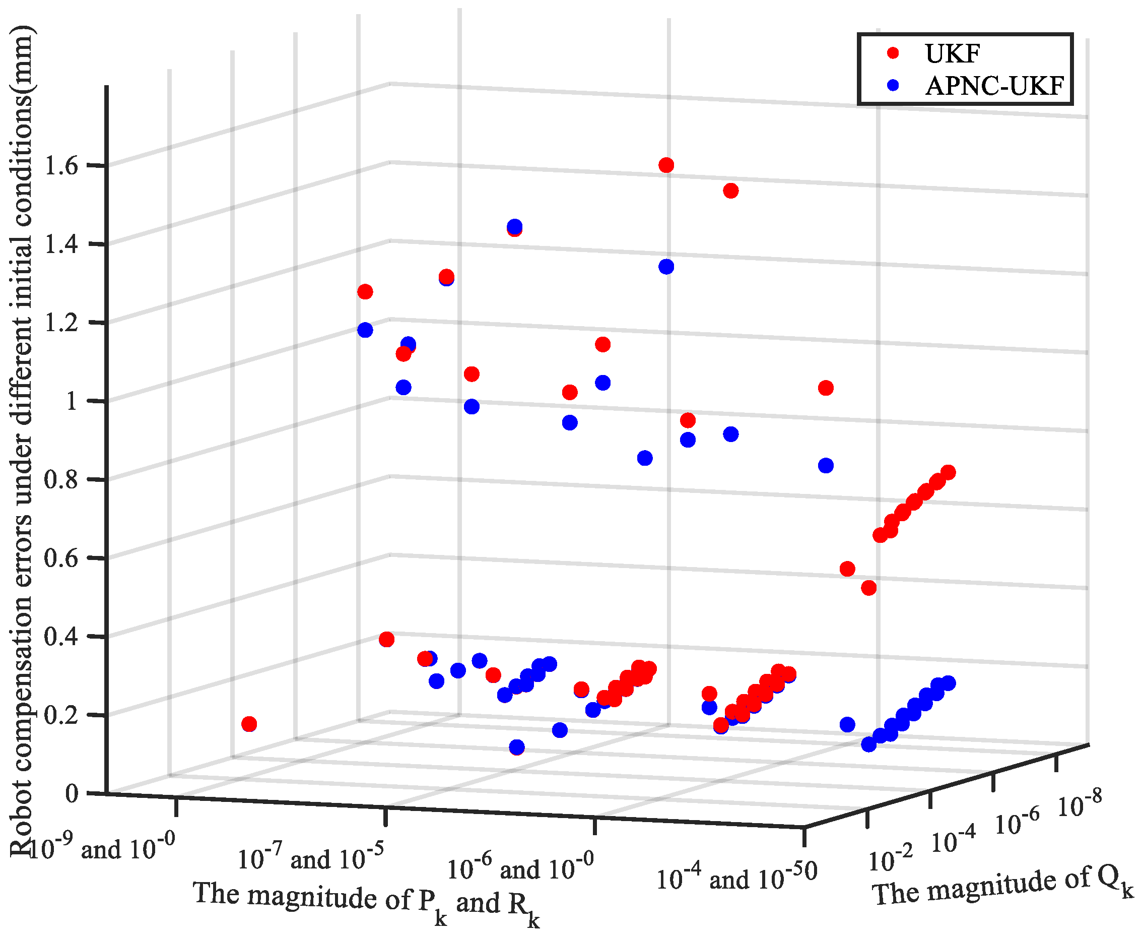
By comparing the conventional UKF and the APNC-UKF with different initial parameters, the stability of APNC-UKF parameter identification is proved, which can effectively reduce the number of adjustments of initial parameters.

(3)

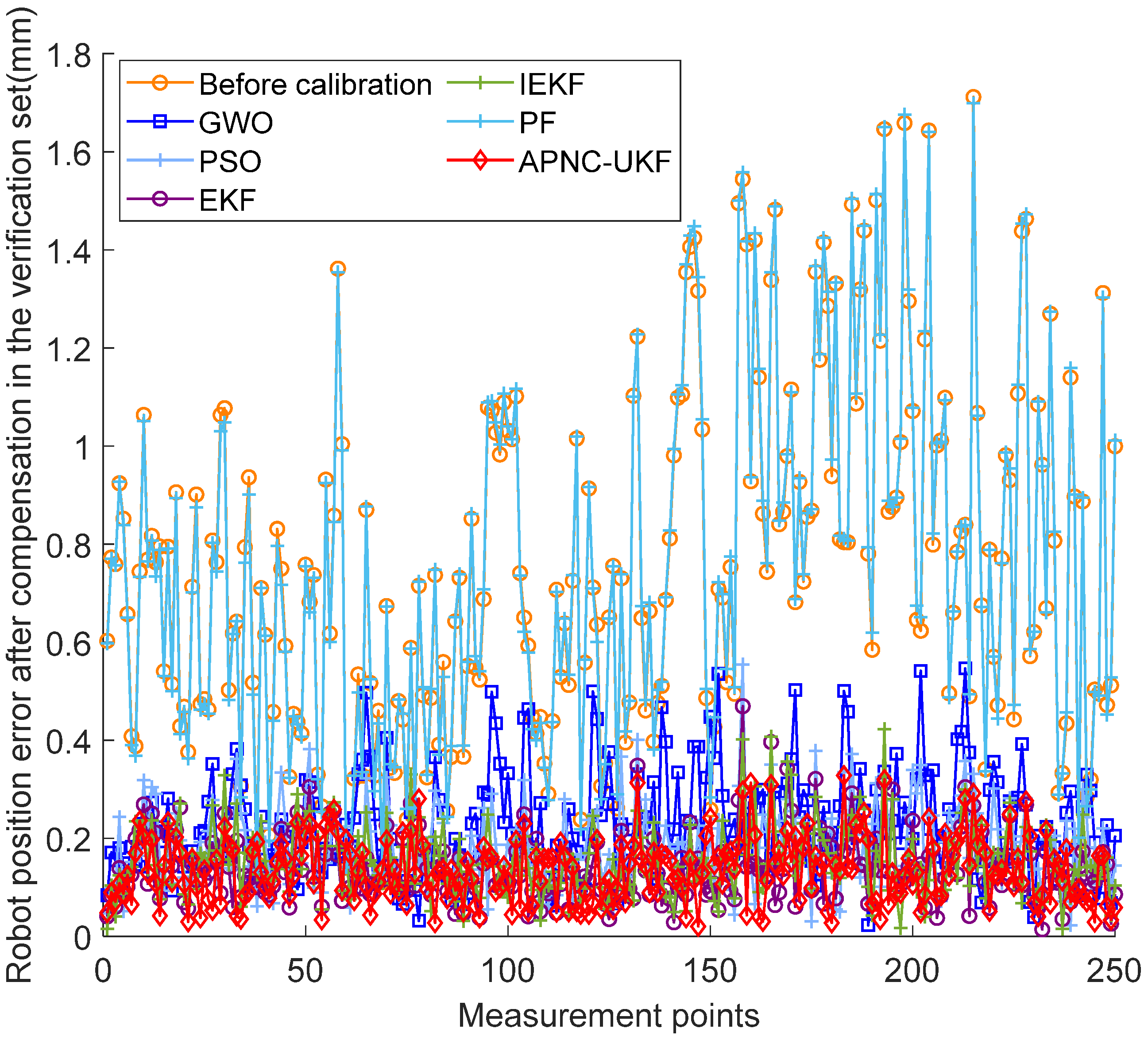
Compared with the EKF, IEKF, PF, PSO, and GWO algorithms commonly used in robot calibration, the APNC-UKF proposed in this paper has advantages in the three indicators of maximum, average value, and standard deviation, and the robot compensation accuracy is higher.

The rest of this paper is organized as follows, Section 2 provides a brief overview of related work on the kinematic and error modeling of robotic calibration systems. Section 3 presents the proposed APNC-UKF algorithm for estimating geometric parameters. Section 4 verifies the effectiveness of the proposed method in experiments by comparing it with four other algorithms. Section 5 concludes the paper.

2. Modeling and Problem Formulation

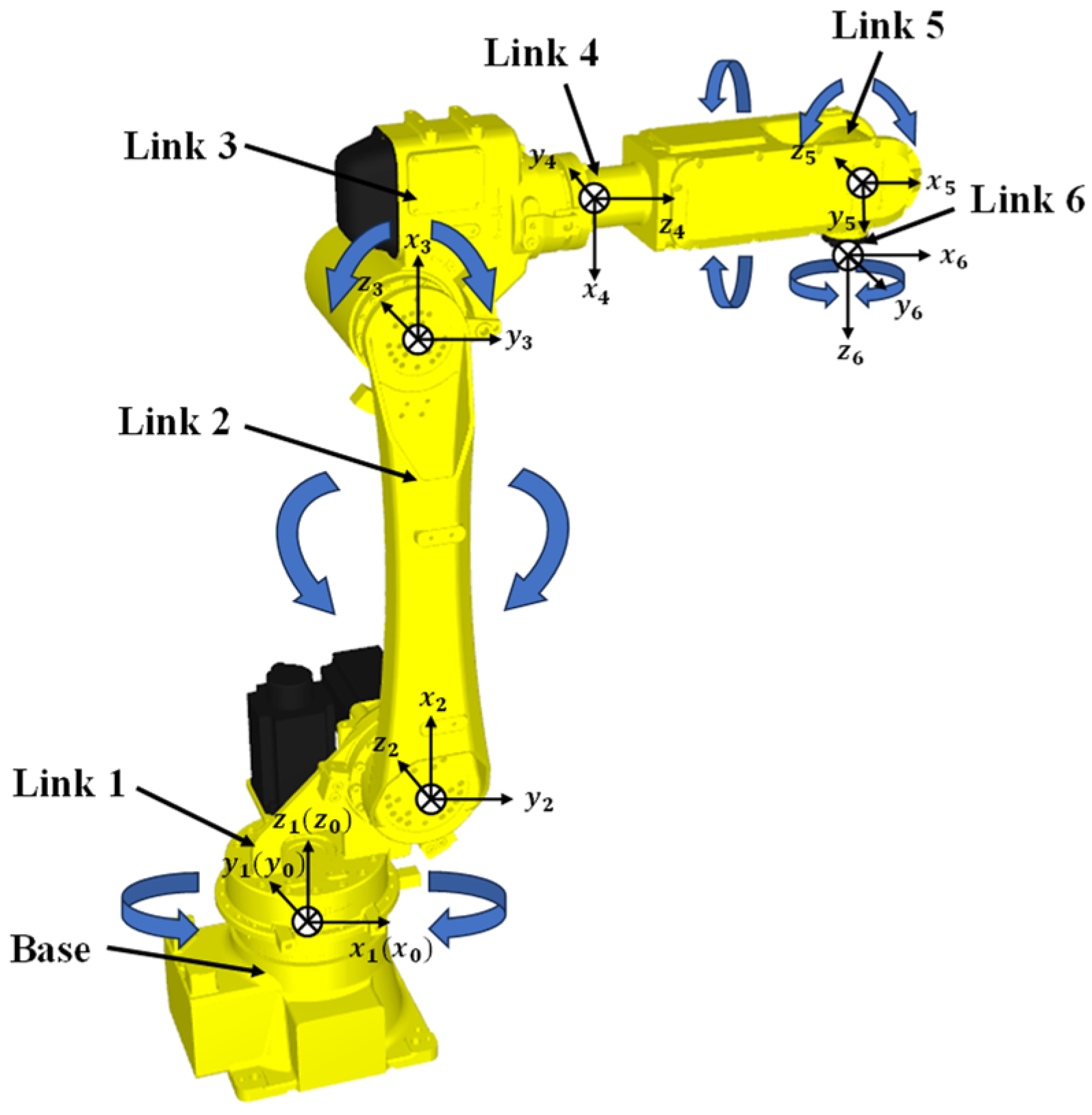
2.1. Robot Kinematic Modeling

This paper uses a 6R general industrial robot as an example to test the proposed method, as shown in Figure 1. Firstly, the robot’s coordinate system is established based on the MD-H method [18]. In turn, the kinematic parameters of the robot are obtained, as shown in

Table 2. The nominal structural parameters of EFORT ER20-C10 robot.

i	αi−1 (°)	ai−1 (mm)	di (mm)	θi (°)
1	0	0	540.000	θ1
2	−90	166.605	0	θ2
3	0	782.270	0	θ3
4	−90	138.826	761.350	θ4
5	90	0	0	θ5
6	0	0	125.000	θ6

, where ${\alpha }_{i-1}$ denotes the link length of joint i − 1, i.e., the length of the common vertical line between joint axis i − 1 and joint axis I; a_i−1 denotes the link twist angle, i.e., the angle between the two axes of axis i − 1 rotating to axis i around a_i−1; θ_i denotes the joint rotation angle of joint i, i.e., the angle between the two adjacent linkages rotating around the common axis; and d_i denotes the link i offset, i.e., the distance along the common axis of two adjacent links.

According to the principle of coordinate homogeneous transformation, the coordinate system relationship between link i − 1 and link i can be represented by the homogeneous transformation matrix ${}_i{}^{i-1}T$:

$$\begin{array}{ll}{}_{i\hspace{1em} }{}^{i-1}T& =\mathrm{Rot}(x,{\alpha }_{i-1})·\mathrm{Trans}(x,a_{i-1})·\mathrm{Rot}(z,{\theta }_i)·\mathrm{Trans}(z,d_i)\\ & =\left[\begin{array}{cccc}1& 0& 0& 0\\ 0& \mathrm{c}{\alpha }_{i-1}& -\mathrm{s}{\alpha }_{i-1}& 0\\ 0& \mathrm{s}{\alpha }_{i-1}& \mathrm{c}{\alpha }_{i-1}& 0\\ 0& 0& 0& 1\end{array}\right]·\left[\begin{array}{cccc}1& 0& 0& a_{i-1}\\ 0& 1& 0& 0\\ 0& 0& 1& 0\\ 0& 0& 0& 1\end{array}\right]·\left[\begin{array}{cccc}\mathrm{c}\theta & -\mathrm{s}\theta & 0& 0\\ \mathrm{s}\theta & \mathrm{c}\theta & 0& 0\\ 0& 0& 1& 0\\ 0& 0& 0& 1\end{array}\right]·\left[\begin{array}{cccc}1& 0& 0& 0\\ 0& 1& 0& 0\\ 0& 0& 1& d_i\\ 0& 0& 0& 1\end{array}\right]\\ & =\left[\begin{array}{cccc}\mathrm{c}{\theta }_i& -\mathrm{s}{\theta }_i& 0& a_{i-1}\\ \mathrm{s}{\theta }_i\mathrm{c}{\alpha }_{i-1}& \mathrm{c}{\theta }_i\mathrm{c}{\alpha }_{i-1}& -\mathrm{s}{\alpha }_{i-1}& -\mathrm{s}{\alpha }_{i-1}{d}_i\\ \mathrm{s}{\theta }_i\mathrm{s}{\alpha }_{i-1}& \mathrm{c}{\theta }_i\mathrm{s}{\alpha }_{i-1}& \mathrm{c}{\alpha }_{i-1}& \mathrm{c}{\alpha }_{i-1}{d}_i\\ 0& 0& 0& 1\end{array}\right]\end{array}$$

(1)

where s represents sin (•) and c represents cos (•). The homogeneous transformation matrix of the robot’s tool center point (TCP) relative to the robot’s base coordinate system (BCS) can be calculated by multiplying the homogeneous transformation matrix between the adjacent links, as shown in (1); then, the position of the robot’s TCP can be obtained by (2).

$${}_6{}^{0}T{=}_1^{0}T{·}_2^{1}T{·}_3^{2}T{·}_4^{3}T{·}_5^{4}T{·}_6^{5}T$$

(2)

2.2. Calibration System Modeling

When using a laser tracker for robot kinematic calibration, the spherical mounted retroreflector (SMR) needs to be mounted on the robot’s end, and the laser tracker collects the position data of the SMR. Thus, the collected data are the position of the SMR in the measuring coordinate system (MCS). Therefore, it is necessary to add the transformation of the BCS to the MCS and the SMR coordinate system to the coordinate system of the robot’s end to (2), which can be modified as:

$${}_{\mathrm{tool} }{}^{\mathrm{word}}T{=}_0^{\mathrm{word}}T{·}_1^{0}T{·}_2^{1}T{·}_3^{2}T{·}_4^{3}T{·}_5^{4}T{·}_6^{5}T·p_{\mathrm{tool}}$$

(3)

where p_tool = [lx, ly, lz, 1]^T represents the position offset of the SMR relative to the robot’s end, and ${}_{0\hspace{1em} }{}^{\mathrm{word}}T$ represents the homogeneous transformation matrix from the robot’s BCS to the MCS:

$$\begin{array}{ll}{}_{0\hspace{1em} }{}^{\mathrm{word}}T& =\mathrm{Rot}(z,\theta )·\mathrm{Rot}(y,\beta )·\mathrm{Rot}(x,\gamma )·\mathrm{Trans}(bx,by,bz)\\ & =\left[\begin{array}{cccc}\mathrm{c}\theta & -\mathrm{s}\theta & 0& 0\\ \mathrm{s}\theta & \mathrm{c}\theta & 0& 0\\ 0& 0& 1& 0\\ 0& 0& 0& 1\end{array}\right]·\left[\begin{array}{cccc}\mathrm{c}\beta & 0& \mathrm{s}\beta & 0\\ 0& 1& 0& 0\\ -\mathrm{s}\beta & 0& \mathrm{c}\beta & 0\\ 0& 0& 0& 1\end{array}\right]·\left[\begin{array}{cccc}1& 0& 0& 0\\ 0& \mathrm{c}\gamma & -\mathrm{s}\gamma & 0\\ 0& \mathrm{s}\gamma & \mathrm{c}\gamma & 0\\ 0& 0& 0& 1\end{array}\right]·\left[\begin{array}{cccc}0& 0& 0& bx\\ 0& 0& 0& by\\ 0& 0& 1& bz\\ 0& 0& 0& 1\end{array}\right]\end{array}$$

(4)

where A, β, and γ represent the rotation angle of the robot’s base coordinate system relative to the z-axis, y-axis, and x-axis of the measurement coordinate system, respectively. bx, by, and bz represent the offset of the origin of the robot‘s BCS relative to the x-axis, y-axis, and z-axis of the MCS, so the entire calibration system contains 33 parameters. However, only 8 (θ₂, θ₃, θ₄, θ₅, a₂, a₃, a₄, d₄) of the 24 parameters of the EFORT ER20-C10 robot are open for users to compensate in the robot controller. Thus, 17 parameters are identified in this paper, including 8 for the robot and 9 for the coordinate system conversion from MCS to the robot’s TCP.

The 6 parameters of the conversion of the MCS and the robot‘s BCS and the 3 parameters of the conversion of the robot end coordinate system and the robot’s TCP coordinate system are generally much larger than the others, so they are identified first. This process is called pre-identification in order to align the MCS and the robot’s TCP. After pre-identification, 17 parameters are identified together, including 8 for the robot and 9 for the coordinate system conversion from MCS to the robot’s TCP. This process is called calibration system parameter identification.

3. Calibration System Parameter Identification Based on APNC-UKF

3.1. Parameter Identification Based on UKF

The UKF is used to obtain the influence of non-linear transformation on state estimation through a set of specially selected sigma points [19]. The UKF is different from the conventional Kalman filter and extended Kalman filter. It does not need to expand the Taylor series of the non-linear function (that is, it does not need to calculate the Jacobian matrix for linearization), so it is easier to implement in the high-dimensional state space. It can retain the information of the high-order term so that the identified parameters are more accurate and the calibrated accuracy of the robot is higher.

$$\{\begin{array}{l}{x}_{k+1}=f_k(x_k)+w_k\\ y_k=h_k(x_k)+v_k\\ w_k~\mathcal{N}(0,Q_k),v_k~\mathcal{N}(0,R_k)\end{array}$$

(5)

where x_k represents the state error of the system at time k, y_k is the measured value of the system, f(•) is the state update function, and h(•) is the observation function; both w_k and v_k are normal distribution white noises with zero mean, and their covariance matrices are Q_k and R_k, respectively.

The main steps of the UKF method are as follows:

(1)

Initialization:

$$P_0^{+}=E[(x_0-{\widehat{x}}_0^{+}){(x_0-{\widehat{x}}_0^{+})}^T]$$

(6)

where ${\widehat{x}}_0^{+}$ is the calibration system parameter error (the initial value is 0) at the previous moment, and its covariance matrix is $P_0^{+}$.

(2)

Cycle k = 1, 2, …, n, and completes the following steps.

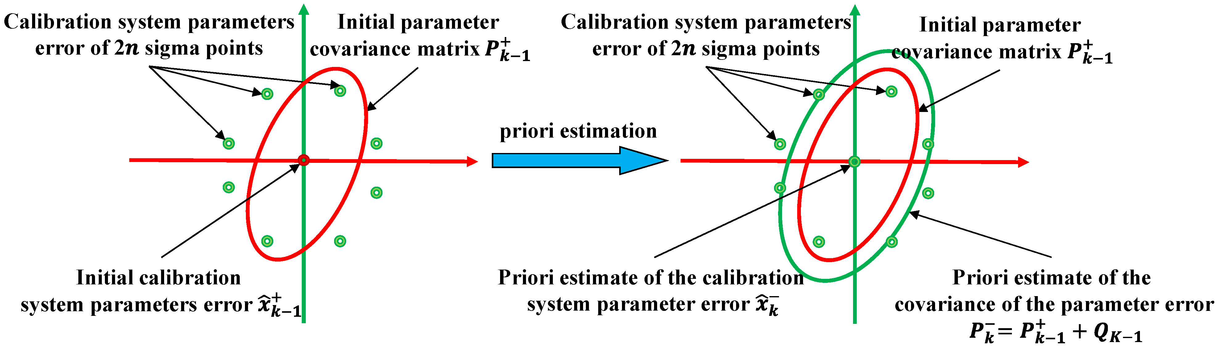
• Select 2n sigma points and obtain 2n priori estimates by non-linear system equations:

$$\{\begin{array}{l}{\tilde{x}}^{(i)}=\{\begin{array}{l}{(\sqrt{n{P}_{k-1}^{+}})}_i^T,i=1,2,\dots ,n\\ -{(\sqrt{n{P}_{k-1}^{+}})}_i^T,i=n+1,n+2,\dots ,2n\end{array}\\ {\widehat{x}}_{k-1}^{(i)}={\widehat{x}}_{k-1}^{+}+{\tilde{x}}^{(i)}\end{array}$$

(7)

$${\widehat{x}}_k^{(i)}=f_k({\widehat{x}}_{k-1}^{(i)})$$

(8)

where n is the dimensions of the calibration system, ${\tilde{x}}^{(i)}$ is the value of 2n sigma points, and ${\widehat{x}}_{k-1}^{(i)}$ is the prior estimate of the parameter of each sigma point at time k − 1. The parameters in the robot calibration are constant. The prior estimate of 2n sigma points at time k remains unchanged after the state update function, so ${\widehat{x}}_{k-1}^{(i)}$ and ${\widehat{x}}_k^{(i)}$ are equal.

b.

Calculate the prior estimation and prior estimation error covariance:

$${\widehat{x}}_k^{-}=\frac{1}{2n}{\displaystyle \sum _{i=1}^{2n}{\widehat{x}}_k^{(i)}}$$

(9)

$$P_k^{-}=\frac{1}{2n}{\displaystyle \sum _{i=1}^{2n}({\widehat{x}}_k^{(i)}-{\widehat{x}}_k^{-}){({\widehat{x}}_k^{(i)}-{\widehat{x}}_k^{-})}^T}+Q_{k-1}$$

(10)

where ${\widehat{x}}_k^{-}$ is the prior estimate of the calibration system parameter error, and $P_k^{-}$ is the prior estimate covariance matrix.

c.

Select 2n sigma points and obtain 2n measured predicted values through the non-linear measurement equation:

$$\{\begin{array}{l}{\tilde{x}}^{(i)}=\{\begin{array}{l}{(\sqrt{n{P}_k^{-}})}_i^T,i=1,2,\dots ,n\\ -{(\sqrt{n{P}_k^{-}})}_i^T,i=n+1,n+2,\dots ,2n\end{array}\\ {\widehat{x}}_k^{(i)}={\widehat{x}}_k^{-}+{\tilde{x}}^{(i)}\end{array}$$

(11)

$${\widehat{y}}_k^{(i)}=h_k(x_{\mathrm{initial}}+{\widehat{x}}_k^{(i)})$$

(12)

where x_initial is the initial parameters of the calibration system. ${\widehat{y}}_k^{(i)}$ is the predicted measurement value obtained by substituting ($x_{initial}+{\widehat{x}}_k^{(i)}$) of 2n sigma into the measurement equation (robot forward kinematic equation).

d.

Calculate measurement estimation, measurement estimation covariance, and cross-covariance:

$$\{\begin{array}{l}{\widehat{y}}_k=\frac{1}{2n}{\displaystyle \sum _{i=1}^{2n}{\widehat{y}}_k^{(i)}}\\ P_y=\frac{1}{2n}{\displaystyle \sum _{i=1}^{2n}({\widehat{y}}_k^{(i)}-{\widehat{y}}_k){({\widehat{y}}_k^{(i)}-{\widehat{y}}_k)}^T}+R_k\\ P_{xy}=\frac{1}{2n}{\displaystyle \sum _{i=1}^{2n}({\widehat{x}}_k^{(i)}-{\widehat{x}}_k^{-}){({\widehat{y}}_k^{(i)}-{\widehat{y}}_k)}^T}\end{array}$$

(13)

where ${\widehat{y}}_k$ is the estimated value of the measurement, $P_y$ is the covariance matrix of ${\widehat{y}}_k$, and $P_{xy}$ is the cross-covariance of ${\widehat{x}}_k^{-}$ and ${\widehat{y}}_k$.

e.

Update posterior state estimation and posterior estimation covariance:

$$\{\begin{array}{l}{K}_k=P_{xy}{P}_y^{-1}\\ {\widehat{x}}_k^{+}={\widehat{x}}_k^{-}+K_k(y_k-{\widehat{y}}_k)\\ P_k^{+}=P_k^{-}-K_k{P}_y{K}_k^T\end{array}$$

(14)

where K_k is the Kalman gain, ${\widehat{x}}_k^{+}$ is the posterior estimate, and $P_k^{+}$ is the covariance matrix of ${\widehat{x}}_k^{+}$.

Finally, the final parameters are obtained by adding the initial parameter $x_{\mathrm{initial}}$ to the iterative geometric parameter error ${\widehat{x}}_k^{+}$.

$$x=x_{\mathrm{initial}}+{\widehat{x}}_k^{+}$$

(15)

3.2. Limitation Analysis of UKF Used in Robot Calibration

According to the steps of Section 3.1, the UKF algorithm can be used to identify the parameter error of the calibration system. 2n sigma points are calculated by (7), in which the parameter error of the calibration system of the first n sigma points and the parameter errors of the calibration system of the last n sigma points are opposite to each other. Since the parameters of the calibration system are all constants, (8) and (9) can be expressed as follows:

$${\widehat{x}}_k^{(i)}=f_k({\widehat{x}}_{k-1}^{(i)})={\widehat{x}}_{k-1}^{(i)}={\widehat{x}}_{k-1}^{+}+{\tilde{x}}^{(i)}$$

(16)

$${\widehat{x}}_k^{-}=\frac{1}{2n}{\displaystyle \sum _{i=1}^{2n}{\widehat{x}}_k^{(i)}}={\widehat{x}}_{k-1}^{+}$$

(17)

which means the prior does not correct the calibration system error parameters. Only the covariance matrix P_k of the parameters is corrected, as shown in Figure 2, and (10) can be expressed as:

$$P_k^{-}=P_{k-1}^{+}+Q_{k-1}$$

(18)

Therefore, the Q_k matrix greatly influences the generation of sigma points in the posterior, which has an essential influence on the measurement estimation value. Through the implementation of the algorithm in Section 3.1, nine parameters of the robot base coordinate system to the coordinate system of the laser tracker are identified, and the P_k matrix in each prior process is recorded.

Figure 3 shows that the order of magnitude of angle and length parameters is very different. The conventional Q_k matrix is a diagonal matrix with the same order of magnitude, so it cannot be applied to robot calibration.

Suppose the Q_k matrix is defined according to the magnitude of the error value of the length parameters. In that case, the Q_k matrix will disturb the angle parameters in each iteration process and cannot converge. Suppose the Q_k matrix is defined according to the magnitude of the angle parameters. In that case, the Q_k matrix has little effect on the convergence of the length parameters, thus weakening the identification accuracy of the UKF algorithm.

3.3. APNC-UKF

The problem with the conventional Q_k matrix is that it cannot be adaptively adjusted by the magnitude of the angle parameter error and the length parameter error, and the magnitude of the angle parameter error and the length parameter error of different robots are unknown. Therefore, only the information in the iterative process of the algorithm can be captured to correct the Q_k matrix. It is known that only a posterior estimation is used to correct the parameter error of the calibration system in each iteration, and the degree of parameter correction in each algorithm iteration is related to the magnitude of the parameter error. Therefore, the magnitude of the parameters can be estimated by the difference between the parameter errors before and after the posterior estimation

$$\delta ={\widehat{x}}_k^{+}-{\widehat{x}}_k^{-}={\left[{\delta }_{angle}\hspace{1em}{\delta }_{length}\right]}^{\mathrm{T}}$$

(19)

where $\delta$ is the difference between the parameters of the prior and the posterior. ${\delta }_{angle}={[{\delta }_{{\theta }_2} {\delta }_{{\theta }_3} {\delta }_{\theta 4} {\delta }_{{\theta }_5} {\delta }_A {\delta }_{\beta } {\delta }_{\gamma }]}^{\mathrm{T}}$ represents the difference in the angle parameters. ${\delta }_{length}={[{\delta }_{a_2} {\delta }_{a_3} {\delta }_{a4} {\delta }_{d_4} {\delta }_{bx} {\delta }_{by} {\delta }_{bz} {\delta }_{lx} {\delta }_{ly} {\delta }_{lz}]}^{\mathrm{T}}$ represents the difference in the length parameters. Due to the unstable convergence of the parameters in the previous algorithm iteration. The ratio of the sum of the angle parameters’ differences to the sum of all parameter differences is used as the weight of the angle parameters, that is, $w_1$, and the weight of the length parameters $w_2$ is the ratio of the sum of the length parameters’ differences to the sum of all parameter differences.

$$w_1={\displaystyle \sum _{J=1}^7{\delta }_{angl{e}_{(J)}}}{({\displaystyle \sum _{J=1}^7{\delta }_{angl{e}_{(J)}}}+{\displaystyle \sum _{L=1}^{10}{\delta }_{lengt{h}_{(L)}}})}^{-1}$$

(20)

$$w_2={\displaystyle \sum _{L=1}^{10}{\delta }_{lengt{h}_{(L)}}}{({\displaystyle \sum _{J=1}^7{\delta }_{angl{e}_{(J)}}}+{\displaystyle \sum _{L=1}^{10}{\delta }_{lengt{h}_{(L)}}})}^{-1}$$

(21)

The specific steps of the improved UKF algorithm are shown in Algorithm 1, in which the Q_k matrix correction formula is expressed as:

$$Q_{angle}=\left[\begin{array}{ccccccc}{Q}_{{\theta }_2}& 0& 0& 0& 0& 0& 0\\ 0& Q_{{\theta }_3}& 0& 0& 0& 0& 0\\ 0& 0& Q_{{\theta }_4}& 0& 0& 0& 0\\ 0& 0& 0& Q_{{\theta }_5}& 0& 0& 0\\ 0& 0& 0& 0& Q_A& 0& 0\\ 0& 0& 0& 0& 0& Q_{\beta }& 0\\ 0& 0& 0& 0& 0& 0& Q_{\gamma }\end{array}\right]$$

(22)

$$Q_{length}=\left[\begin{array}{cccccccccc}{Q}_{a_2}& 0& 0& 0& 0& 0& 0& 0& 0& 0\\ 0& Q_{a_3}& 0& 0& 0& 0& 0& 0& 0& 0\\ 0& 0& Q_{a_4}& 0& 0& 0& 0& 0& 0& 0\\ 0& 0& 0& Q_{d_4}& 0& 0& 0& 0& 0& 0\\ 0& 0& 0& 0& Q_{bx}& 0& 0& 0& 0& 0\\ 0& 0& 0& 0& 0& Q_{by}& 0& 0& 0& 0\\ 0& 0& 0& 0& 0& 0& Q_{bz}& 0& 0& 0\\ 0& 0& 0& 0& 0& 0& 0& Q_{lx}& 0& 0\\ 0& 0& 0& 0& 0& 0& 0& 0& Q_{ly}& 0\\ 0& 0& 0& 0& 0& 0& 0& 0& 0& Q_{lz}\end{array}\right]$$

(23)

$$Q_k=\left[\begin{array}{cc}{Q}_{angle}& 0\\ 0& Q_{length}\end{array}\right]\ast \left[\begin{array}{cccccc}{w}_1& 0& 0& 0& 0& 0\\ 0& \ddots & 0& 0& 0& 0\\ 0& 0& w_1& 0& 0& 0\\ 0& 0& 0& w_2& 0& 0\\ 0& 0& 0& 0& \ddots & 0\\ 0& 0& 0& 0& 0& w_2\end{array}\right]$$

(24)

where Q_angle represents the process noise covariance matrix of the angle parameters. Q_length represents the process noise covariance matrix of the length parameters. The values of the Q_angle and Q_length matrix diagonal are all values initialized by the Q_k matrix, which are adjusted by w₁ and w₂ during the iteration process.

Algorithm 1 APNC-UKF
/∗Initialization∗/
1 Initialize P0, Q0 and R0
2 Initialize $w_1=1$ and $w_2=1$
3 Initialize ${\widehat{x}}_{k-1}^{+}=x_0$
/∗ APNC-UKF Step∗/
for k = 1, 2, …n
	select prior sigma points ${\tilde{x}}^{(i)}$ via (7)
	Calculate ${\widehat{x}}_k^{-}$ base on (9)
	Calculate $Q_k$ base on (24)
	Calculate $P_k^{-}$ base on (10) and Updated Qk
	select posterior sigma points ${\tilde{x}}^{(i)}$ via (11)
	Calculate ${\widehat{y}}_k$, $P_y$ and $P_{xy}$ base on (13)
	Update $K_k$, ${\widehat{x}}_k^{+}$ and $P_k^{+}$ with (14)
	Calculate $\delta$, $w_1$ and $w_2$ base on (19) (20) (21)
end for

The magnitude of the angle parameters is very small, w₂ is almost close to 1, so the magnitude of the Q_k matrix initialization is based on the length parameter error magnitude, and the angle parameters’ magnitude of the Q_k matrix is adaptively adjusted by the weight w₁. In general, the length parameter error of the robot is in the order of 0.1 mm, so the order of ${\tilde{x}}^{(i)}$ added to the prior estimate ${\widehat{x}}_k^{-}$ by the sigma point in (11) should be in the order of 0.1 mm. Through (18), the order of magnitude of the $P_k^{-}$ matrix can be calculated to be 1 × 10⁻⁴, so, the magnitude of the initial Q_k matrix is more appropriate to take 1 × 10⁻⁴. Alternatively, it can be observed from Figure 3b that the length parameters of the P_k matrix are around 1 × 10⁻³ or 1 × 10⁻⁴. To ensure convergence accuracy, choosing 1 × 10⁻⁴ for the $Q_k$ matrix is the optimal selection.

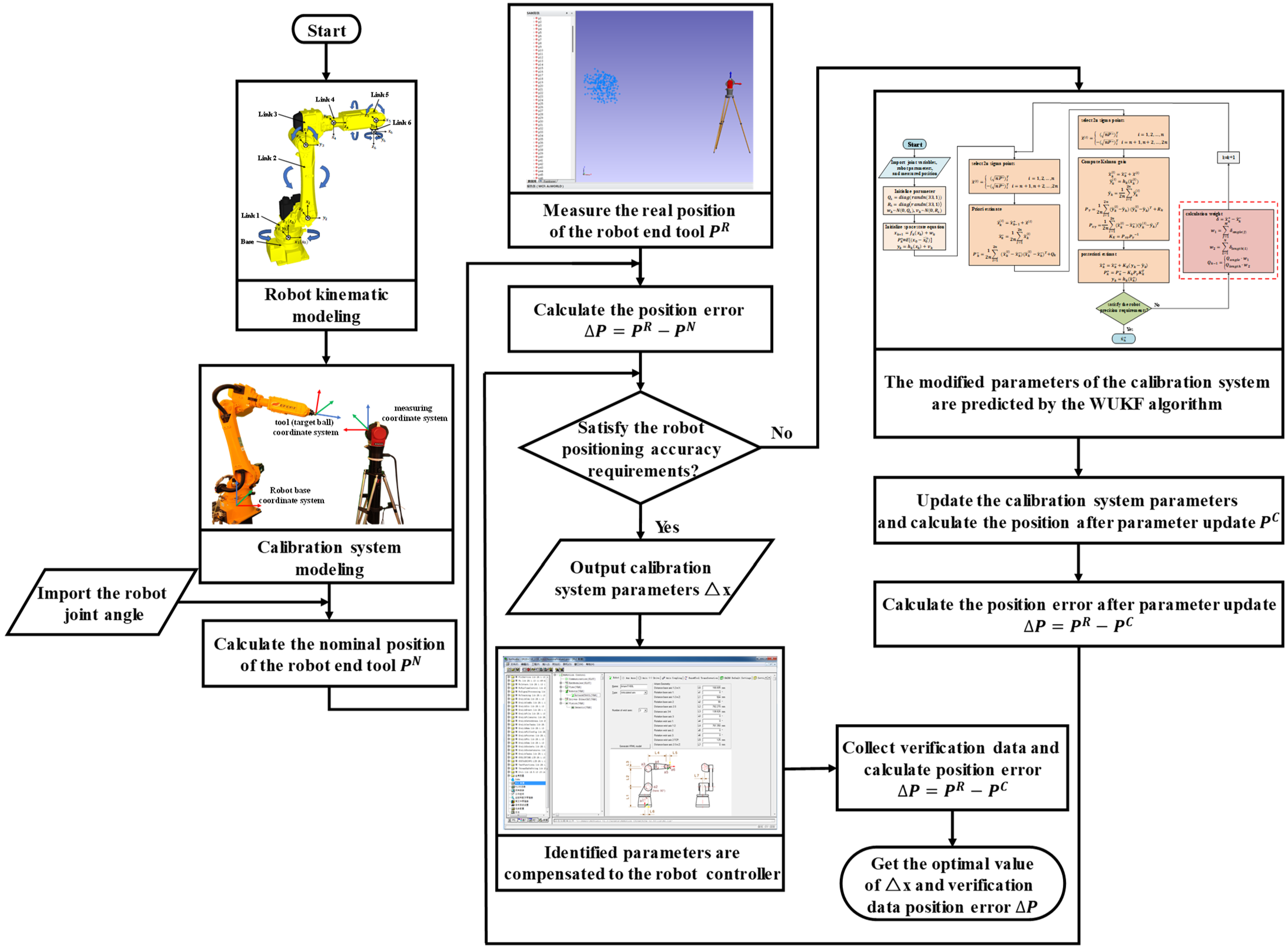
4. Experiments

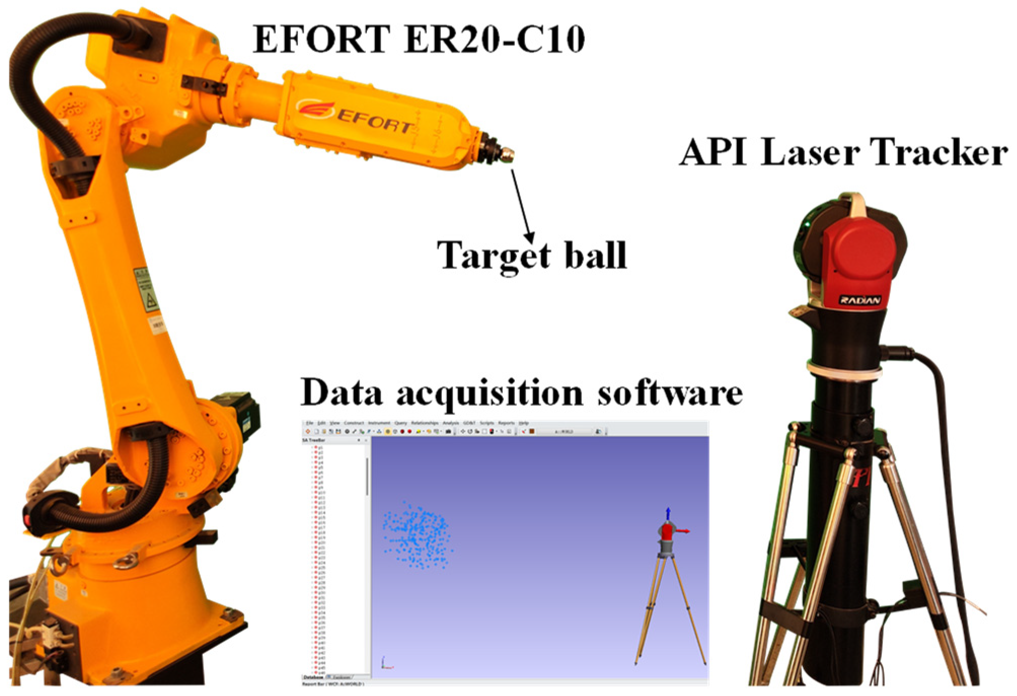
4.1. Experimental Settings

• Data Acquisition.

As shown in Figure 4, this paper uses a laser tracker to collect data sets for the EFORT ER20-C10 robot. In this experiment, a total of 300 sets of sample data of the robot are planned. The measurement range of the laser tracker typically ranges from 2 m to 50 m. In this paper, there is an approximate distance deviation of 4 m between the robot’s BCS and the MCS. By aligning the coordinate systems, the offset in the x-, y-, and z-directions between the two coordinate systems is approximately 3854 mm, 411 mm, and 888 mm. The data collection range is within a cubic volume of 600 mm × 600 mm × 600 mm. In the robot’s base coordinate system, the range is shown in

Table 3. The data collection range.

	x-Direction (mm)	y-Direction (mm)	z-Direction (mm)
max value	1350	800	950
min value	750	200	350

:

b.

Experimental steps.

(1)

The position of the robot’s TCP is collected by the laser tracker and Spatial Analyzer (SA) of version 2017.08.11_29326(x64), and the joint angle of the robot is exported by the robot controller.

(2)

Fifty sets of joint angles and positions are selected as the identification set data, and the parameter error obtained by parameter identification is compensated to the controller of the robot. Then, the parameters of the robot are corrected, and the accuracy of the robot is improved.

(3)

The laser tracker and SA software are used to collect the remaining 250 sets of data, and the robot accuracy before and after kinematic parameter identification and compensation is compared.

c.

Evaluation protocol.

The three evaluation indicators of maximum, mean, and standard deviation are widely used to evaluate the performance of the calibration model involved, and they are primarily practiced in [20,21,22].

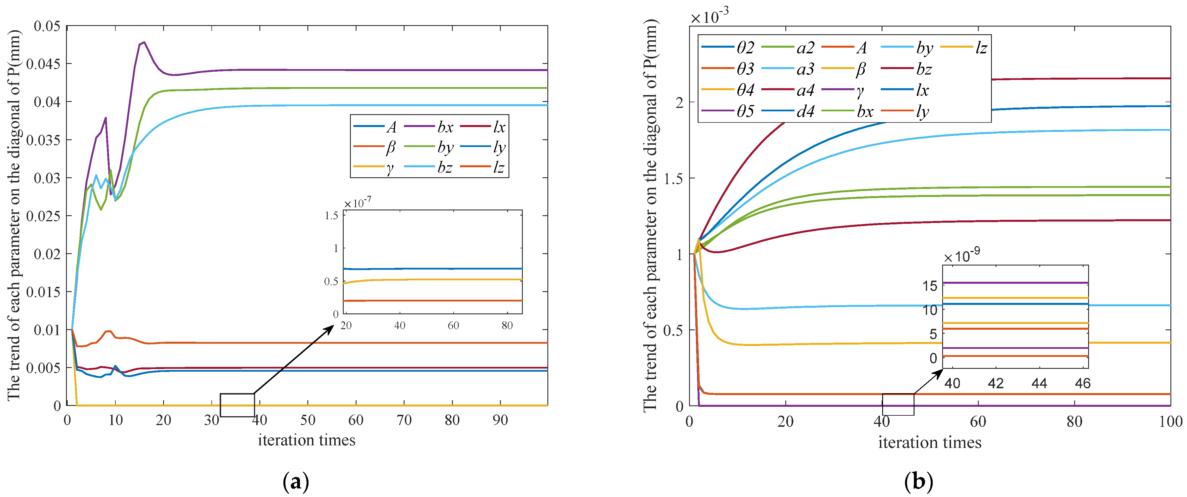
4.2. Adaptive Strategy Validation

In the UKF algorithm, P_k, Q_k, and R_k are the three covariance matrices that need to be input into the system. By adjusting their values, the best effect of the system can be obtained. Therefore, different P_k, Q_k, and R_k values greatly influence the accuracy of the robot system’s identification. In this section, the three matrices of P_k, Q_k, and R_k are valued from ten orders of magnitude of 1 × 10⁻⁰, 1 × 10⁻¹, 1 × 10⁻² … and 1 × 10⁻⁹, and then arranged and combined to identify the parameter error of the robot calibration system for 1000 times. Then, the effects of the APNC-UKF and conventional UKF are compared. Due to the open root formula in the UKF algorithm, some P_k, Q_k, and R_k combinations cannot complete the parameter identification, and some of the identification results of the P_k, Q_k, and R_k combinations do not converge. After calibration, the robot’s accuracy is several hundred millimeters, so these parameter combinations should be eliminated. Only the combination of the robot accuracy within 1 mm after the parameter identification of the conventional UKF and the APNC-UKF is retained, and there are 66 groups of combination results. As shown in Figure 5, the accuracy of the APNC-UKF has been improved compared to the parameter identification accuracy of the UKF, and the specific values are shown in Appendix A.

The APNC-UKF under nine sets of parameter combinations is less effective than the conventional UKF algorithm, but the gap of eight groups is less than 1%, and only one group has a gap of 54.66%. In general, the identification results of the APNC-UKF are more stable, and the identification accuracy can be reduced to less than 0.2 mm in 53 sets of parameter combinations. In 57 sets of parameter combinations, the APNC-UKF has different degrees of improvement compared with the conventional UKF algorithm, so the effectiveness of the proposed method can be proved. It can be seen that when the magnitude of the Q_k matrix is 1 × 10⁻⁴, the improvement of the conventional UKF algorithm is more stable, which is the same as the theory of Section 3.3.

4.3. Performance Evaluation

There are several standard calibration algorithms for performance verification for validating the virtues of the proposed APNC-UKF calibration algorithm:

(1)

M1: GWO is widely used in non-linear non-Gaussian dynamical systems for robot calibration [12].

(2)

M2: PSO is a classical optimization algorithm widely applied to solve various engineering problems [11].

(3)

M3: The EKF is used to solve non-linear state estimation problems and has been successfully applied to non-linear robot calibration systems [15].

(4)

M4: The IEKF algorithm is an improved version of the Kalman filter used for state estimation in non-linear systems [16].

(5)

M5: The PF is a probabilistic and statistical method that is mainly used to solve uncertainty problems. It is a sample-based filtering method that estimates the state of a system by generating a large number of random particles. [14].

(6)

M6: The APNC-UKF algorithm proposed in this study.

Each of the above algorithms iterates to the parameter convergence to obtain the identification result of the parameter, and the identified parameters are compensated by the robot controller. Figure 6 depicts the absolute position error of the validation data set before and after compensation by M1–6.

Table 4. Errors after compensation with different algorithms.

	Algorithms	Before Calibration	GWO	PSO	EKF	IEKF	PF	APNC -UKF
Metrics
Max (mm)		1.7117	0.5466	0.5547	0.4694	0.4227	1.6986	0.3282
Mean (mm)		0.7558	0.2306	0.1832	0.1405	0.1544	0.7581	0.1347
Std (mm)		0.3479	0.1049	0.0826	0.0702	0.0723	0.3518	0.0669

quantifies the results of the parameter compensation by different algorithms in the verification set.

Based on the compensation accuracy of the robot, the following findings can be obtained: M4’s max, mean, and std errors reach 0.3282 mm, 0.1347 mm, and 0.0669 mm, respectively, which are 80.82%, 82.18%, and 80.78% lower than the corresponding errors. The max error of the APNC-UKF is significantly lower than the corresponding errors of M1, M2, M3, M4, and M5 by 39.96%, 40.83%, 30.08%, 22.35%, and 80.68%, respectively, the mean error is lower than the corresponding errors of M1, M2, M3, M4, and M5 by 41.59%, 26.47%, 4.13%, 12.76%, and 82.23%, respectively, and the std error is lower than the corresponding errors of M1, M2, M3, M4, and M5 by 36.22%, 19.01%, 4.71%, 7.67%, and 80.98%, respectively.

Compared with the intelligent optimization algorithms M1 and M2, the numerical optimization algorithms M3 and M4 iterate on the Jacobian matrix, which is an extension of the gradient descent method and does not have the risk of falling into local optimization, so the compensation effect is better. The linearization of the Jacobian matrix causes the M3, M4, and M5 methods to lose some information, while the UKF keeps the information of the higher-order terms by fitting the Jacobian matrix with sigma points. Although different P_k, Q_k, and R_k parameters significantly influence the UKF’s effect, the proposed method can make the UKF’s effect more stable. Hence, the compensation parameters are more stable in the robot workspace. The full-text work is shown in Figure 7. After the parameter identification process, parameters can be compensated using the official compensation software for the EFORT ER20-C10 robot. In the software, ‘a’ represents angular parameters, ‘L’ represents length parameters, ‘a2’, ‘a3’, ‘a4’, and ‘a5’ represent θ₂, θ₃, θ₄, and θ₅, respectively, and ‘L6’, ‘L2’, and ‘L3’ represent a₂, a₃, and a₄. ‘L4’ represents d₄. Initially, these eight parameters are adjusted to the values identified, then input into the robot. Finally, the robot is restarted to complete the parameter compensation process.

5. Conclusions

This paper proposes a UKF algorithm based on adaptive process noise covariance for robot calibration systems. The robot calibration system is constant, and the prior estimate of the system is the same as the last posterior estimate. This leads to a more significant impact of the process noise covariance matrix Q_k on the accuracy of parameter identification, thus affecting the robot’s accuracy after compensation. Thus, in this paper, a kinematic model of a 6-degree-of-freedom robot is established based on the MD-H rule. Then, to solve the problem that the conventional Q_k matrix in the UKF algorithm interferes with the convergence of different magnitude parameters, an adaptive strategy is proposed to correct Q_k matrix. Finally, the APNC-UKF is compared with the EKF, IEKF, PF, PSO, and GWO algorithms, and the results show that the effectiveness of the adaptive strategy and the compensation accuracy of the APNC-UKF are higher than those of other robot calibration systems.

References

- Fu, P.; Miao, Y.; Wang, Y.; Jiang, X.; Xu, C.; Liu, L.; Zhou, L. A Review of Research Progress and Key Technologies of Robotic Drilling in Aviation. CAAI Trans. Intell. Syst. 2022, 17, 874–885. [Google Scholar]
- Gao, G.; Niu, J.; Liu, F.; Na, J. Positioning Error Compensation of 6-Dof Robots Based on Anisotropic Error Similarity. Opt. Precis. Eng. 2022, 30, 1955–1967. [Google Scholar] [CrossRef]
- Zhang, C.T.; Wang, Y. Research on Online Calibration Method of Six-Axis Force Sensor for Industrial Robot. J. Electron. Meas. Instrum. 2021, 35, 161–168. [Google Scholar]
- Feng, L.M.; Yu, J.H.; Wang, Y.Y. Research on Calibration of Absolute Positioning Accuracy of 6-Dof Cooperative Robot. Manuf. Autom. 2022, 44, 25–28. [Google Scholar]
- Ni, H.K.; Yang, Z.Y.; Yang, Y.F. Robot Kinematics Calibration Method Considering Base Frame Error. China Mech. Eng. 2021, 33, 647–655. [Google Scholar]
- Sun, T.; Liu, C.Y.; Lian, B.B. Calibration for Precision Kinematic Control of an Articulated Serial Robot. IEEE Trans. Ind. Electron. 2021, 68, 6000–6009. [Google Scholar] [CrossRef]
- Guo, Y.L.; Zou, L.; Wang, Z.L. A Novel Kinematic Parameters Calibration Method for Industrial Robot Based on Levenberg-Marquardt and Differential Evolution Hybrid Algorithm. Robot. Comput.-Integr. Manuf. 2021, 71, 161–165. [Google Scholar]
- Ping, Y.; Guo, Z.G.; Yang, B.K. Plane Kinematic Calibration Method for Industrial Robot Based on Dynamic Measurement of Double Ball Bar. Precis. Eng. 2021, 62, 265–272. [Google Scholar]
- Jiang, Z.Z.; Zhou, J.; Han, H.Q. A Novel Robot Hand-Eye Calibration Method to Enhance Calibration Accuracy Based on the Poe Model. Adv. Robot. 2023, 37, 1052–1062. [Google Scholar] [CrossRef]
- Bai, M.; Zhang, M.L.; Zhang, H. Calibration Method Based on Models and Least-Squares Support Vector Regression Enhancing Robot Position Accuracy. IEEE Access 2021, 9, 136060–136070. [Google Scholar] [CrossRef]
- Wang, W.D.; Song, H.J.; Yan, Z.Y. A Universal Index and an Improved Pso Algorithm for Optimal Pose Selection in Kinematic Calibration of a Novel Surgical Robot. Robot. Comput.-Integr. Manuf. 2021, 50, 90–101. [Google Scholar] [CrossRef]
- Peng, T.C.; Zhang, T.; Sun, Z.J. Research on Robot Accuracy Compensation Method Based on Modified Grey Wolf Algorithm. In Proceedings of the 2023 8th Asia-Pacific Conference on Intelligent Robot Systems, Xi’an, China, 7–9 July 2023; pp. 1–6. [Google Scholar]
- Lv, H.Y. Application of Process Noise Recursive Least Squares Method. China Instrum. 2021, 1, 1–6. [Google Scholar]
- Deng, X.; Ge, L.; Li, R.; Liu, Z. Research on the Kinematic Parameter Calibration Method of Industrial Robot Based on Lm and Pf Algorithm. 2020. Available online: https://www.semanticscholar.org/paper/Research-on-the-kinematic-parameter-calibration-of-Deng-Ge/fdf9bf2b7c0beece8302fdd9ce5140a648700d2f (accessed on 22 August 2020).
- Le, N.V.; Caverly, R.J. Cable-Driven Parallel Robot Pose Estimation Using Extended Kalman Filtering with Inertial Payload Measurements. IEEE Robot. Autom. Lett. 2021, 6, 3615–3622. [Google Scholar]
- Lee, K.; Kwon, H.; You, K. Iterative Solution of Relative Localization for Cooperative Multi-Robot Using Iekf. Univers. J. Mech. Eng. 2017, 5, 15–19. [Google Scholar] [CrossRef]
- Du, G.L.; Shao, H.K.; Chen, Y.J. An Online Method for Serial Robot Self-Calibration with Cmac and Ukf. Robot. Comput.-Integr. Manuf. 2016, 42, 39–48. [Google Scholar] [CrossRef]
- Urrea, C.; Agramonte, R. Evaluation of Parameter Identification of a Real Manipulator Robot. Symmetry 2022, 14, 1446. [Google Scholar] [CrossRef]
- Geetha, S.; Natarajan, U. Kinematic Parameter Estimation of Vrt 6 Robot Using Unscented Kalman Filter with Adaptive Choice of Scaling Parameter. J. Balk. Tribol. Assoc. 2018, 24, 123–140. [Google Scholar]
- Huang, T.; Zhao, D.; Yin, F.W. Kinematic Calibration of a 6-Dof Hybrid Robot by Considering Multicollinearity in the Identification Jacobian. Mech. Mach. Theory 2019, 131, 371–384. [Google Scholar] [CrossRef]
- Li, M.Y.; Du, Z.J.; Ma, X.X. A Robot Hand-Eye Calibration Method of Line Laser Sensor Based on 3d Reconstruction. Robot. Comput.-Integr. Manuf. 2021, 71, 102–106. [Google Scholar] [CrossRef]
- Li, Z.B.; Li, S.; Bamasag, O.O. Diversified Regularization Enhanced Training for Effective Manipulator Calibration. IEEE Trans. Neural Netw. Learn. Syst. 2023, 34, 8778–8790. [Google Scholar] [CrossRef] [PubMed]