Fault-Tolerant Control Study of Four-Wheel Independent Drive Electric Vehicles Based on Drive Actuator Faults

Abstract

Failure of any of the drive systems in a Four-Wheel Independent Drive (4WID) electric vehicle may affect the control performance and driving safety of the whole vehicle. Therefore, in this paper, a fault-tolerant controller (FTC) for 4WID electric vehicles considering drive actuator failures is proposed. First, a comprehensive characterization of multiple fault types is achieved by establishing a generalized fault model and designing a comprehensive fault factor. Second, based on the comprehensive fault factor, an LPV model with faults is constructed. Further, a fault-tolerant controller based on LPV/H∞ output feedback is designed by combining the weighting function. Finally, the effectiveness of the FTC in this paper is verified by simulation and hardware-in-the-loop (HIL) experiments. The experimental results show that the FTC designed in this paper can improve the stability of the vehicle traveling while ensuring tracking accuracy when the drive system fails.

1. Introduction

With the increasingly serious problems of the energy crisis and environmental pollution, electric vehicles have become one of the effective ways to solve these problems, and 4WID electric vehicles have occupied an important position in the field of electric vehicles due to their unique advantages. 4WID electric vehicles, as an important branch of electric vehicles, represent an important direction for the development of future automobile technology [1]. Since the driving force of each wheel can be controlled independently, 4WID electric vehicles excel in handling performance. The stability and safety of the vehicle can be maintained both at high speeds and low-speed cornering [2,3]. At the same time, this design also allows the vehicle to better adapt to various road conditions, including slippery, rugged, and other complex road conditions. However, it is difficult to avoid the objective existence of failure risk completely. For example, when the drive actuator of a wheel fails, the absence of an effective FTC strategy may lead to the loss of control of the vehicle or a dangerous situation. To reduce the risk of failure and improve the safety of vehicles, it is essential to study fault-tolerant control strategies. By designing a reasonable FTC strategy, when a wheel drive actuator fails, the driving force of other wheels can be adjusted to compensate for the influence of the failed wheel, to maintain the stability and driving safety of the whole vehicle.

The main goal of FTC is to ensure the security and stability of the system, as well as an acceptable level of performance, in the event of a failure or malfunction of one or more critical components of the system [4,5,6]. In an FTC system, when a failure is detected, it can maintain its normal functionality by reconfiguring the control policy or utilizing backup resources. FTC can be divided into two main categories: active FTC (AFTC) and passive FTC (PFTC) [7]. AFTC can proactively deal with failures occurring in the system by reconfiguring the controller or making adjustments to the controller parameters based on real-time fault information fed back from the system but requires higher detection accuracy as well as complex real-time computations [8,9]. In contrast, PFTC reacts to a set of assumed failure modes; the design is fixed and gives robustness only to this assumed set of failure modes without the need for fault detection and diagnosis [10]. Therefore, PFTC is more advantageous than AFTC in practical applications [11].

In the field of vehicle engineering, adaptive control [12], sliding mode control [13], fuzzy control [14], robust control [15,16,17], LPV control, and FTC strategies combining multiple control methods are widely used [18,19,20]. Among them, robust control aims to uphold the stability and optimal performance of a system, despite the uncertainties and variabilities inherent in its parameters [21,22]. LPV control usually approximates a nonlinear system as a time-varying linear system [23], providing technical support for the design of fault-tolerant controllers. In [24], a fault-tolerant control strategy based on H∞ robustness is proposed for the lateral stability control of 4WID electric vehicles with uncertain parameters in the event of actuator and sensor failures. In [25], a novel fault-tolerant control strategy, grounded in LPV control principles, is introduced to address the damper fault challenges encountered in semi-active suspension systems. When both the actuator and sensor fail simultaneously, Raouaa Tayari et al. designed a robust AFTC strategy based on LPV control [26]. Through the above analysis, FTC plays a crucial role in the stable operation and driving safety of the vehicle when the vehicle sensor or actuator fails.

As the actuator of the drive system of 4WID electric vehicles, the hub motor will directly affect the normal operation and driving safety of the vehicle in the case of failure [27,28]. In [29], a fault-tolerant stabilization control algorithm including torque distribution and stability control is proposed for keeping the motor healthy in response to the motor or inverter failure problem in 4WID electric vehicles. In [30], a fault-tolerant control algorithm based on optimal allocation is proposed for the faulty 4WID electric vehicle actuator problem to ensure the safety of vehicle operation. Aiming at the problem that the cooperative control of the drive system and steering system cannot be fully considered when the motor fails, a model-free 4WID adaptive AFTC strategy for electric vehicles with multiple inputs and multiple outputs has been proposed [31].

Based on the above analysis, FTC strategies for 4WID electric vehicle drive systems mainly focus on fault-tolerant control by redistributing drive forces [32,33]. However, this type of strategy usually pays little attention to the effect of the fault itself on the performance of the FTC [34]. It may affect the control performance of fault-tolerant controllers under specific fault conditions and thus requires further research and optimization [35]. To address the fault problem of drive actuators, this paper investigates three common fault types, i.e., add-on faults, failure faults, and stuck-at faults [36,37], establishes a generalized fault model encompassing multiple drive actuators, and subsequently crafts fault factors tailored specifically for these actuators. Secondly, the generalized fault model was used to design a comprehensive fault factor for both sides of the vehicle, which was used to determine the state of the drive system so that the drive torque could be distributed efficiently. Then, a FTC based on LPV/H∞ output feedback is designed to assure the stability and safety of the 4WID electric vehicles when the drive actuator fails.

The main contributions of this paper are as follows:

(1) A FTC based on LPV/H∞ output feedback is proposed to address the fault problem of the drive actuator of 4WID electric vehicles. Compared with the H∞ output feedback control strategy that does not consider the changing parameters, the controller designed in this paper can better improve the stability and safety of the vehicle when the drive actuator fails;

(2) This paper develops a generalized fault model for drive actuators and characterizes the state of the drive system of 4WID electric vehicles using a comprehensive fault factor for both sides of the designed vehicle. A polyhedral LPV model with four vertices is developed and weighting functions are introduced by using the integrated fault factor as variation parameters. Finally, based on the output feedback, the linear matrix inequality is solved to obtain the integrated controller.

2. Vehicle Dynamic Model

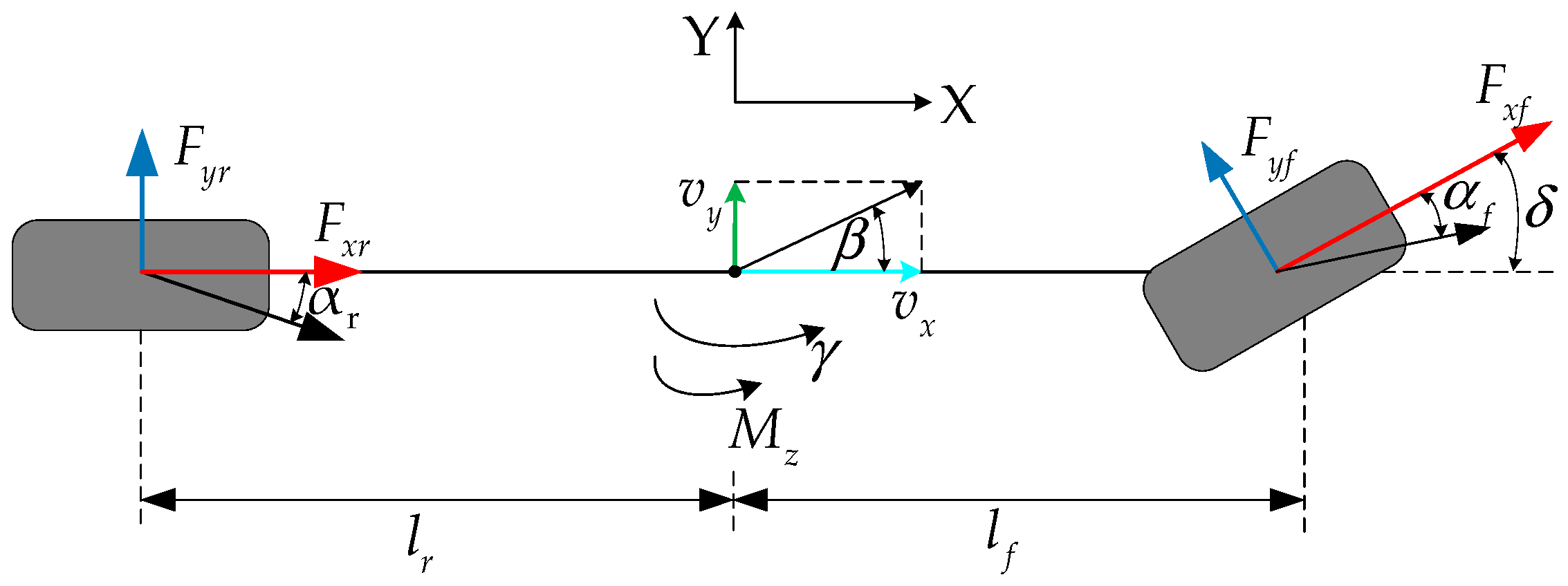
2.1. Two-Degree-of-Freedom Vehicle Dynamics Model

Under the assumption that the wheelbase of the vehicle is equal, the mechanical characteristics of the tires are consistent, and the steering wheels have equal turning angles, the vertical, pitch, and roll spatial movements of the vehicle are ignored, and the air resistance in the driving process is considered to establish a two-degree-of-freedom dynamics model of 4WID electric vehicles [38]. A simplified model of the car is shown in Figure 1.

First, the kinematic equations of the longitudinal and yaw directions of the vehicle are established [39]:

$${\dot{v}}_x=\gamma v_y-\frac{1}{m}\left(C_a{v}_x^2-F_x\right)$$

(1)

$$\dot{\gamma }=\frac{1}{I_z}\left(l_f{F}_{yf}\cos \delta -l_r{F}_{yr}+M_z\right)$$

(2)

where $v_x$ and $v_y$ represent the speed of the vehicle in the longitudinal and lateral directions, respectively; $m$ is the total mass; $\gamma$ stands for yaw rate; $I_z$ represents the moment of inertia; $C_a$ indicates the coefficient of air resistance; $l_f$ and $l_r$ represent the distance from the center of mass of the vehicle to the front and rear axles, respectively; $\delta$ is the front wheel angle; $F_x$ is the total longitudinal force of the driving wheel; $M_z$ is the additional yaw moment; $F_{yf}$ represents the lateral force on the front side wheel; and $F_{yr}$ represents the lateral force on the rear side wheel.

The total wheel longitudinal force and additional yaw moment in Equations (1) and (2) can be expressed by Equations (3) and (4):

$$F_x=\left(F_{xfl}+F_{xfr}\right)\cos \delta +F_{xrl}+F_{xrr}$$

(3)

$$M_z=\left(F_{xfl}+F_{xfr}\right)l_f\sin \delta -\left(F_{xfl}-F_{xfr}\right)l_s\cos \delta -F_{xrl}{l}_s+F_{xrr}{l}_s$$

(4)

where $F_{ii}$ represents the longitudinal force of the wheel $\left(i=fl, rl, fr, rr\right)$ and $l_s$ is half the wheelbase. Torque is calculated as positive to the left and counterclockwise. The calculation of driving torque for each driving wheel is as follows:

$$T_i=R_t{F}_{xi}$$

(5)

where $T_i$ represents the driving torque of the wheel and $R_t$ is the rolling radius of the wheel.

From the linear tire model:

$$F_{yi}=C_i{\alpha }_i, i=f,r$$

(6)

where $C_i$ represents the lateral stiffness of the wheel and ${\alpha }_i$ represents the side deflection angle of the wheel. According to the small angle theorem, the front and rear wheel side angles can be described as [40]

$$\left\{\begin{array}{l}{\alpha }_f=\frac{1}{v_x}\left(-\gamma l_f-v_y\right)+\delta \\ {\alpha }_r=\frac{1}{v_x}\left(\gamma l_r-v_y\right)\end{array}\right.$$

(7)

Using the sum of the vehicle’s left-hand wheel torque and the sum of the right-hand wheel torque as control variables, it can be described as

$$\left\{\begin{array}{l}{u}_1=T_{fl}\cos \delta +T_{rl}\\ u_2=T_{fr}\cos \delta +T_{rr}\end{array}\right.$$

(8)

In combination with Equations (1)–(8), the kinematic equations of the vehicle can be re-expressed as:

$$\left\{\begin{array}{l}{\dot{v}}_x=\gamma v_y-\frac{C_a{v}_x}{m}{v}_x+\frac{1}{m{R}_t}\left(u_1+u_2\right)\\ \dot{\gamma }=\frac{\left(C_r{l}_r-C_f{l}_f\right)v_y}{v_x^2{I}_z}-\frac{C_f{l}_f^2+C_r{l}_r^2}{v_x{I}_z}\gamma +\frac{C_f{l}_f}{I_z}\delta +\frac{l_s}{I_z{R}_t}\left(-u_1+u_2\right)\end{array}\right.$$

(9)

According to Formula (9), the dynamic state-space model of the vehicle is represented as:

$${\dot{x}}_0=A_0{x}_0+B_{\delta }\delta +B_{u}u$$

(10)

where ${x_0=\left[v_x,\gamma \right]}^T$, ${u=\left[u_1,u_2\right]}^T$,

$$A_0=\left[\begin{array}{cc}-\frac{C_a{v}_x}{m}& v_y\\ \frac{\left(C_r{l}_r-C_f{l}_f\right)v_y}{v_x^2{I}_z}& -\frac{C_f{l}_f^2+C_r{l}_r^2}{v_x{I}_z}\end{array}\right], B_{\delta }=\left[\begin{array}{c}0\\ \frac{C_f{l}_f}{I_z}\end{array}\right], B_u=\left[\begin{array}{cc}\frac{1}{m{R}_t}& \frac{1}{m{R}_t}\\ -\frac{l_s}{R_t{I}_z}& \frac{l_s}{R_t{I}_z}\end{array}\right]$$

The desired longitudinal rate and yaw rate are introduced as $x_d={\left[v_{xd}, {\gamma }_d\right]}^T$ and the new state vector redefined:

$$x={\left[{\left(x_0-x_d\right)}^T, {\left({\displaystyle {\int }_0^t\left(x_0-x_d\right)dt}\right)}^T\right]}^T$$

(11)

Thus, an augmented system can be obtained:

$$\dot{x}=Ax+B_1\varpi +B_{2}u$$

(12)

where $A=\left[\begin{array}{cc}{A}_0& 0\\ I_1& 0\end{array}\right], B_1=\left[\begin{array}{ccc}{B}_{\delta }& A_0& -I_1\\ 0& 0& 0\end{array}\right], B_2=\left[\begin{array}{c}{B}_u\\ 0\end{array}\right], \varpi ={\left[\begin{array}{ccc}\delta & x_d& {\dot{x}}_d\end{array}\right]}^T$, and $\varpi$ is the amount of system interference.

2.2. Tracking Model

Vehicle road tracking refers to the design of control inputs for a system that enables a vehicle to track a desired trajectory at a desired speed according to the relevant control theory. Therefore, the vehicle road tracking model can be represented by the following formula [41]:

$$\left\{\begin{array}{l}\dot{e}=v_x\sin \psi +v_y\cos \psi \\ e_p=e+L\sin \psi \\ \dot{\psi }={\dot{\psi }}_r-{\dot{\psi }}_d=\gamma -\rho v_x\end{array}\right.$$

(13)

where $e$ is the lateral offset; $\psi$ is the course angle error; ${\dot{\psi }}_r$ is the actual course angle; ${\dot{\psi }}_d$ is the expected course angle; $L$ is the pre-sight distance; $e_p$ is the previewing error at the previewing point; and $\rho$ is the curvature of the road.

Based on the classical two-degree-of-freedom model, combined with the road tracking model, the vehicle–road error dynamics model is established, and the corresponding controller can be solved by using the LQR method to obtain the front wheel angle required in this paper, which is expressed as follows:

$$\delta =k\xi +{\delta }_b$$

(14)

where $k$ is the matrix of feedback coefficients; $\xi$ is the state quantity, including lateral offset $e$, lateral offset rate of change $\dot{e}$, heading angle error $\psi$, and heading angle error rate of change $\dot{\psi }$; and ${\delta }_b$ is the cornering compensation quantity, ${\delta }_b=\rho \left(L-l_{r}k\left(3\right)-\frac{m{v}_x}{L}\left(\frac{l_r}{C_f}\right)+\frac{l_f\left(k\left(3\right)-1\right)}{C_r}\right)$.

2.3. Vehicle Expected Yaw Speed Reference Model

The reference model is used to describe the desired traverse angular velocity of the vehicle during traveling. Based on the driving task and road conditions, the desired driving trajectory is determined, and then combined with the vehicle dynamics equations, the desired traverse angular velocity is calculated, so the desired traverse angular velocity reference model can be described as

$${\gamma }_d=\frac{v_x}{L\left(1+K{v}_x^2\right)}\delta$$

(15)

where $L=l_f+l_r$ is the distance from the front axle to the rear axle and $K=\frac{m}{L^2}\left(\frac{l_r}{C_f}-\frac{l_f}{C_r}\right)$ is the stability factor.

2.4. Vertical Load Dynamics Model of the Wheel

Vertical loads are used to determine the maximum drive torque for each wheel and accordingly distribute the drive torque appropriately to the individual drive wheels. Because the load is constantly transferred when driving, the vertical load is described as [42]:

$$\left\{\begin{array}{l}{F}_{zfl}=\frac{m}{2L}\left(g{l}_r-{\dot{v}}_x{h}_g-h_g{l}_r\frac{{\dot{v}}_y+v_x\gamma }{l_s}\right)\\ F_{zfr}=\frac{m}{2L}\left(g{l}_r-{\dot{v}}_x{h}_g+h_g{l}_r\frac{{\dot{v}}_y+v_x\gamma }{l_s}\right)\\ F_{zrl}=\frac{m}{2L}\left(g{l}_r+{\dot{v}}_x{h}_g-h_g{l}_r\frac{{\dot{v}}_y+v_x\gamma }{l_s}\right)\\ F_{zrr}=\frac{m}{2L}\left(g{l}_r+{\dot{v}}_x{h}_g+h_g{l}_r\frac{{\dot{v}}_y+v_x\gamma }{l_s}\right)\end{array}\right.$$

(16)

where $F_{zi}$ represents the vertical load of the wheel $\left(i=fl, rl, fr, rr\right)$; $g$ is the gravitational acceleration; and $h_g$ is the height of the vehicle’s center of mass.

3. Drive Actuator Fault Model

When the partial drive motor of the drive system fails, the actual motor torque control signal will be greatly different from the expected motor output torque control signal, so the following actuator fault model can be established:

$$\left\{\begin{array}{l}{u}_1={\lambda }_1{u}_{d1}+\Delta u_1\\ u_2={\lambda }_2{u}_{d2}+\Delta u_2\end{array}\right.$$

(17)

where ${\lambda }_i\in \left[0,1\right]$ is the combined failure factor for one side of the vehicle; $u_{di}$ is the sum of the desired unilateral moments; and $\Delta u_i$ is additional faults $\left(i=1,2\right)$.

The driving torque ratio of each wheel is expressed as:

$$T_i={\phi }_i{T}_{di}+\Delta T_i$$

(18)

where ${\phi }_i$ is the fault factor of the actuator, representing the severity of the fault of the actuator. $T_{di}$ is the expected torque value of the actuator and $\Delta T_i$ indicates an additional fault.

The fault model described in Equation (16) can be divided into four different fault conditions: (1) ${\phi }_i=1, {\lambda }_i=1, \Delta u_i=0$, no fault; (2) ${\phi }_i=1, {\lambda }_i=1, \Delta u_i \ne 0$, additional fault; (3) ${\phi }_i\in \left(0,1\right), {\lambda }_i\in \left(0,1\right), \Delta u_i=0$ or ${\phi }_i\in \left(0,1\right), {\lambda }_i\in \left(0,1\right), \Delta u_i \ne 0$, failure fault; (4) ${\phi }_i=0, {\lambda }_i=0, \Delta u_i=k$, stuck fault.

The sum of the left and right desired torques $u_{d1}$, $u_{d2}$ can be described as

$$\left\{\begin{array}{l}{u}_{d1}=T_{dfl}\cos \delta +T_{drl}\\ u_{d2}=T_{dfr}\cos \delta +T_{drr}\end{array}\right.$$

(19)

The driving torque distribution laws for the front and rear wheels are designed as follows:

$$\epsilon =\frac{T_{dfl}}{T_{drl}}=\frac{T_{dfr}}{T_{drr}}$$

(20)

By combining Formula (8) and Formulas (16)–(19), the synthetic fault factors and additional faults on both sides of the vehicle can be introduced.

$$\left\{\begin{array}{l}{\lambda }_1=\frac{{\phi }_{fl}\epsilon \cos \delta +{\phi }_{rl}}{1+\epsilon \cos \delta }\\ \Delta u_1=\Delta T_{fl}\cos \delta +\Delta T_{rl}\end{array}\right.$$

(21)

$$\left\{\begin{array}{l}{\lambda }_2=\frac{{\phi }_{fr}\epsilon \cos \delta +{\phi }_{rr}}{1+\epsilon \cos \delta }\\ \Delta u_2=\Delta T_{rl}\cos \delta +\Delta T_{rr}\end{array}\right.$$

(22)

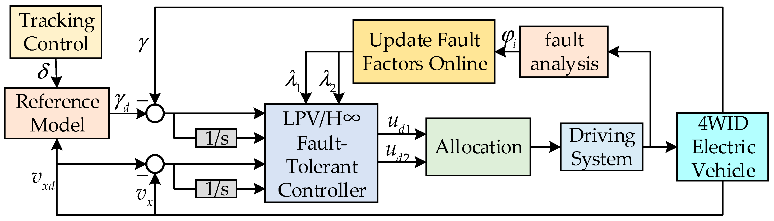
4. Fault-Tolerant Controller Design

The LPV/H∞ fault-tolerant controller is a proposed control strategy for dynamic systems possessing parameter uncertainty and the possibility of faults. This design approach improves the robustness and fault-tolerant performance of the system by considering the variation of the system parameters as a time variable, which is incorporated into the model during the design of the controller. The fault-tolerant control strategy scheme is shown in Figure 2.

4.1. LPV Model

Taking the combined failure factor of both sides of the vehicle as a variation parameter, Equation (10) can be described as the LPV model.

$$\dot{x}=Ax+B_1\varpi +B_2\Gamma \left(\lambda \right)u_d+B_2\Delta u$$

(23)

where $\Gamma \left(\lambda \right)=\mathit{diag}\left\{{\lambda }_1,{\lambda }_2\right\}$, $u_d={\left[u_{d1},u_{d2}\right]}^T, \Delta u={\left[\Delta u_1,\Delta u_2\right]}^T$.

Based on the LPV/H∞ control theory, a reasonable weighting function is designed to make the system maintain good performance and robustness in the face of disturbances and uncertainties of different frequencies.

(I) Longitudinal rate error weighting function $W_{\Delta v}$:

$$W_{\Delta v}=\frac{1}{E{T}_1}\frac{T_{1}s+2\pi f_1}{s+2\pi f_1}$$

(24)

where $T_1$ is the maximum allowed steady-state error, $T_1=0.1$, $E$ is the peak sensitivity, $E=2$, and $f_1$ is the cut-off frequency of longitudinal rate error, $f_1=0.1$.

(II) Expected yaw rate follows the error weighting function $W_{\Delta \gamma }$:

$$W_{\Delta \gamma }=\frac{1}{E{T}_2}\frac{T_{2}s+2\pi f_2}{s+2\pi f_2}$$

(25)

where $T_2=0.1$, $E=2$, $f_2=0.1$.

(III) Left driving torque weighting function $W_{u_{d1}}$:

$$W_{u_{d1}}=\frac{s+{\omega }_3}{T_3+10{\omega }_3}$$

(26)

where $T_3=0.1$ and ${\omega }_3$ is the response bandwidth, ${\omega }_3=100$.

(IV) Right driving torque weighting function $W_{u_{d2}}$:

$$W_{u_{d2}}=\frac{s+{\omega }_4}{T_4+10{\omega }_4}$$

(27)

where $T_4=0.1$, ${\omega }_4=100$.

Combined with the designed weighting function, Equation (22) can be augmented into the following form:

$$\left\{\begin{array}{l}\dot{\zeta }=\overline{A}\zeta +{\overline{B}}_1\sigma +{\overline{B}}_2(\lambda )u_d\\ z={\overline{C}}_1\zeta +{\overline{D}}_{11}\sigma +{\overline{D}}_{12}{u}_d\\ y={\overline{C}}_2\zeta +{\overline{D}}_{21}\sigma +{\overline{D}}_{22}{u}_d\end{array}\right.$$

(28)

where $\zeta$ is the augmented state vector, $\sigma$ is the system disturbance vector, $u_d$ is the control inputs, $u_d={\left[u_{d1},u_{d2}\right]}^T$, $z$ is the weighted controlled outputs vector, $z={\left[z_1, z_2, z_3, z_4\right]}^T$, and $y$ is the system output vector, $y={\left[{\Delta v}_x, \Delta \gamma , {\dot{\Delta v}}_x, \dot{\Delta \gamma }\right]}^T$.

Note that to satisfy the assumptions of the LPV/H∞ control theory that the time-varying parameters cannot depend on matrix 1, the problem can be solved by applying a prefilter to the control inputs [43]. The new control inputs are defined as shown below:

$$\left\{\begin{array}{l}{\dot{x}}_u=A_u{x}_u+B_u\widehat{u}\\ u=C_u{x}_u\end{array}\right.$$

(29)

where $A_u$ is the stable matrix.

As a result, LPV models are widely used:

$$\left\{\begin{array}{l}\dot{\tilde{x}}=\tilde{A}\tilde{x}+{\tilde{B}}_1\sigma +{\tilde{B}}_2(\lambda )u_d\\ z={\tilde{C}}_1\tilde{x}+{\tilde{D}}_{11}\sigma +{\tilde{D}}_{12}{u}_d\\ y={\tilde{C}}_2\tilde{x}+{\tilde{D}}_{21}\sigma +{\tilde{D}}_{22}{u}_d\end{array}\right.$$

(30)

where $\tilde{x}=\left[\begin{array}{c}\zeta \\ x_u\end{array}\right], \tilde{A}=\left[\begin{array}{cc}\overline{A}& {\overline{B}}_2(\lambda )C_u\\ 0& A_u\end{array}\right], {\tilde{B}}_1=\left[\begin{array}{c}{\overline{B}}_1\\ 0\end{array}\right], {\tilde{B}}_2=\left[\begin{array}{c}0\\ B_u\end{array}\right]$, ${\tilde{C}}_1=\left[\begin{array}{cc}{\overline{C}}_1& {\overline{D}}_{12}{C}_u\end{array}\right],$ ${\tilde{C}}_2=\left[\begin{array}{cc}{\overline{C}}_2& 0\end{array}\right], {\tilde{D}}_{11}=0, {\tilde{D}}_{12}={\overline{D}}_{12}, {\tilde{D}}_{21}=0, {\tilde{D}}_{22}=0$.

4.2. LPV/H∞ Output Feedback Fault-Tolerant Controller Design

Based on the LPV multicell type theory and H∞ theory, an output feedback control rate K is designed to include the fault factor λ:

$$K\left(\lambda \right)\left\{\begin{array}{l}{\dot{x}}_k=A_k(\lambda )x_k+B_k(\lambda )y\\ u=C_k(\lambda )x_k+D_k(\lambda )y\end{array}\right.$$

(31)

By bringing the controller $K\left(\lambda \right)$ into Equation (28), the closed-loop system can be obtained:

$$\left\{\begin{array}{l}{\dot{x}}_{kl}=A_{kl}{x}_{kl}+B_{kl}\sigma \\ z=C_{kl}{x}_{kl}+D_{kl}\sigma \end{array}\right.$$

(32)

Constraining the H∞ norm of the closed-loop transfer function to ${‖H‖}_{\infty }<\gamma$ is helpful to enhance the robustness of the system and play a role in resisting disturbances. According to the bounded real theorem [44], the closed-loop system in Equation (32) is stable and the H∞ paradigm of the closed-loop transfer function is less than $\gamma$ if and only if there exists a positive definite matrix $P$ satisfying the following inequality:

$$\left[\begin{array}{ccc}{A}_{kl}^{T}P+P{A}_{kl}& P{B}_{kl}& C_{kl}^T\\ B_{kl}^{T}P& -\gamma I& D_{kl}^T\\ C_{kl}& D_{kl}& -\gamma I\end{array}\right]<0, P>0$$

(33)

4.3. Control Rate Solving

The positive definite matrix $P$ and its inverse matrix $P^{-1}$ are written as follows:

$$P=\left[\begin{array}{cc}Y& N\\ N^T& \ast \end{array}\right], P^{-1}=\left[\begin{array}{cc}X& M\\ M^T& \ast \end{array}\right]$$

(34)

thus, the following equation can be obtained:

$$P{\tau }_1={\tau }_2$$

(35)

as defined below:

$${\tau }_1=\left[\begin{array}{cc}X& I\\ M^{\mathrm{T}}& 0\end{array}\right], {\tau }_2=\left[\begin{array}{cc}I& Y\\ 0& N^{\mathrm{T}}\end{array}\right]$$

(36)

The inequality in Equation (32) is first multiplied by left and right by the diagonal matrices $\mathit{diag}\left({\tau }_1^T, I, I\right)$ and $\mathit{diag}\left({\tau }_1, I, I\right)$, and then by congruent transformations to obtain the matrix inequality shown below:

$$\left\{\begin{array}{l}\left[\begin{array}{cccc}\tilde{A}X+X{\tilde{A}}^{\mathrm{T}}+{\tilde{B}}_2{\widehat{C}}_k+{\left({\tilde{B}}_2{\widehat{C}}_k\right)}^{\mathrm{T}}& {{\widehat{A}}_k}^{\mathrm{T}}+\left(\tilde{A}+{\tilde{B}}_2{\widehat{D}}_k{\tilde{C}}_2\right)& {\tilde{B}}_1+{\tilde{B}}_2{\widehat{D}}_k{\tilde{D}}_{21}& {\left({\tilde{C}}_{1}X+{\tilde{D}}_{12}{\widehat{C}}_k\right)}^{\mathrm{T}}\\ {\widehat{A}}_k+{\left(\tilde{A}+{\tilde{B}}_2{\widehat{D}}_k{\tilde{C}}_2\right)}^{\mathrm{T}}& {\tilde{A}}^{\mathrm{T}}Y+Y\tilde{A}+{\widehat{B}}_k{\tilde{C}}_2+{\left({\widehat{B}}_k{\tilde{C}}_2\right)}^{\mathrm{T}}& Y{\tilde{B}}_1+{\widehat{B}}_k{\tilde{D}}_{21}& {\left({\tilde{C}}_1+{\tilde{D}}_{12}{\widehat{D}}_k{\tilde{C}}_2\right)}^{\mathrm{T}}\\ {\left({\tilde{B}}_1+{\tilde{B}}_2{\widehat{D}}_k{\tilde{D}}_{21}\right)}^{\mathrm{T}}& {\left(Y{\tilde{B}}_1+{\widehat{B}}_k{\tilde{D}}_{21}\right)}^{\mathrm{T}}& -\gamma I& {\left({\tilde{D}}_{11}+{\tilde{D}}_{12}{\widehat{D}}_k{\tilde{D}}_{21}\right)}^{\mathrm{T}}\\ {\tilde{C}}_{1}X+{\tilde{D}}_{12}{\widehat{C}}_k& {\tilde{C}}_1+{\tilde{D}}_{12}{\widehat{D}}_k{\tilde{C}}_2& {\tilde{D}}_{11}+{\tilde{D}}_{12}{\widehat{D}}_k{\tilde{D}}_{21}& -\gamma I\end{array}\right]<0\\ \left[\begin{array}{cc}X& I\\ I& Y\end{array}\right]>0\end{array}\right.$$

(37)

The controller $K$ is solved by solving the linear matrix inequality and the deformed controller coefficient matrix is defined as follows:

$$\left\{\begin{array}{l}{\widehat{A}}_k=N{A}_k{M}^{\mathrm{T}}+Y{\tilde{B}}_2{C}_k{M}^{\mathrm{T}}+N{B}_k{\tilde{C}}_{2}X+Y\left(\tilde{A}+{\tilde{B}}_2{D}_k{\tilde{C}}_2\right)X\\ {\widehat{B}}_k=N{B}_k+Y{\tilde{B}}_2{D}_k\\ {\widehat{C}}_k=C_k{M}^{\mathrm{T}}+D_k{\tilde{C}}_{2}X\\ {\widehat{D}}_k=D_k\end{array}\right.$$

(38)

From Equation (34), it can be deduced that:

$$M{N}^T=I-XY$$

(39)

To calculate the matrix coefficients of the controller, $M, N$ can be solved by the method of singular value decomposition so that it satisfies the inequality (32).

Finally, by solving the linear matrix inequality (35), the controller coefficient matrix of vertices $A_{ki}$, $B_{ki}$, $C_{ki}$ and $D_{ki}$ can be described as

$$\left\{\begin{array}{l}{D}_{ki}={\widehat{D}}_{ki}\\ C_{ki}=\left({\widehat{C}}_{ki}-D_{ki}{\tilde{C}}_{2}X\right)M^{-\mathrm{T}}\\ B_{ki}=N^{-1}\left({\widehat{B}}_{ki}-Y{\tilde{B}}_2{D}_{ki}\right)\\ A_{ki}=N^{-1}\left[\widehat{A}-Y\left(\tilde{A}+{\tilde{B}}_2{D}_{ki}{\tilde{C}}_2\right)X\right]M^{-\mathrm{T}}-N^{-1}Y{\tilde{B}}_2{C}_{ki}-B_{ki}{\tilde{C}}_{2}X{M}^{-\mathrm{T}}\end{array}\right.$$

(40)

Based on the solution of the optimal H∞ controller for the output feedback of each polycell vertex of the LPV system, combined with the polycell theory, the integrated controller of the LPV system can be obtained:

$$K\left(\lambda \right)={\alpha }_1{K}_1+{\alpha }_2{K}_2+{\alpha }_3{K}_3+{\alpha }_4{K}_4$$

(41)

where $K_i$ is the feedback gain of each polycell-type vertex.

The weight function corresponding to the vertices of each polycell type is expressed as

$$\left\{\begin{array}{l}{\alpha }_1=\left|{\lambda }_1-{\lambda }_{1\max }\right|\left|{\lambda }_2-{\lambda }_{2\max }\right|/\Delta \lambda \\ {\alpha }_2=\left|{\lambda }_1-{\lambda }_{1\max }\right|\left|{\lambda }_2-{\lambda }_{2\min }\right|/\Delta \lambda \\ {\alpha }_3=\left|{\lambda }_1-{\lambda }_{1\min }\right|\left|{\lambda }_2-{\lambda }_{2\max }\right|/\Delta \lambda \\ {\alpha }_4=\left|{\lambda }_1-{\lambda }_{1\min }\right|\left|{\lambda }_2-{\lambda }_{2\min }\right|/\Delta \lambda \end{array}\right.$$

(42)

where $\Delta \lambda =\left({\lambda }_{1\max }-{\lambda }_{1\min }\right)\left({\lambda }_{2\max }-{\lambda }_{2\min }\right)$; the weight function needs to be calculated online based on real-time fault factors.

4.4. Driver Distribution Scheme

The upper fault-tolerant controller calculates the sum of the driving torque on both sides of the vehicle. In this paper, a driving torque distribution strategy is designed by combining the vertical load of the wheels and the maximum driving torque.

The maximum driving torque of the driving wheel can be described as:

$$T_{ij\max }=R_t\mu F_{zij}$$

(43)

The wheel expected driving torque distribution strategy is as follows:

$$\left\{\begin{array}{l}{T}_{dfl}=\min \left(\frac{F_{zfl}}{F_{zfl}+F_{zrl}}{u}_{d1},T_{11\max }\right)\\ T_{dfr}=\min \left(\frac{F_{zfr}}{F_{zfr}+F_{zrr}}{u}_{d2},T_{12\max }\right)\\ T_{drl}=\min \left(\frac{F_{zrl}}{F_{zfl}+F_{zrl}}{u}_{d1},T_{21\max }\right)\\ T_{drr}=\min \left(\frac{F_{zrr}}{F_{zfr}+F_{zrr}}{u}_{d2},T_{22\max }\right)\end{array}\right.$$

(44)

The actual wheel torque with a fault can be obtained by combining this with the Formula (17).

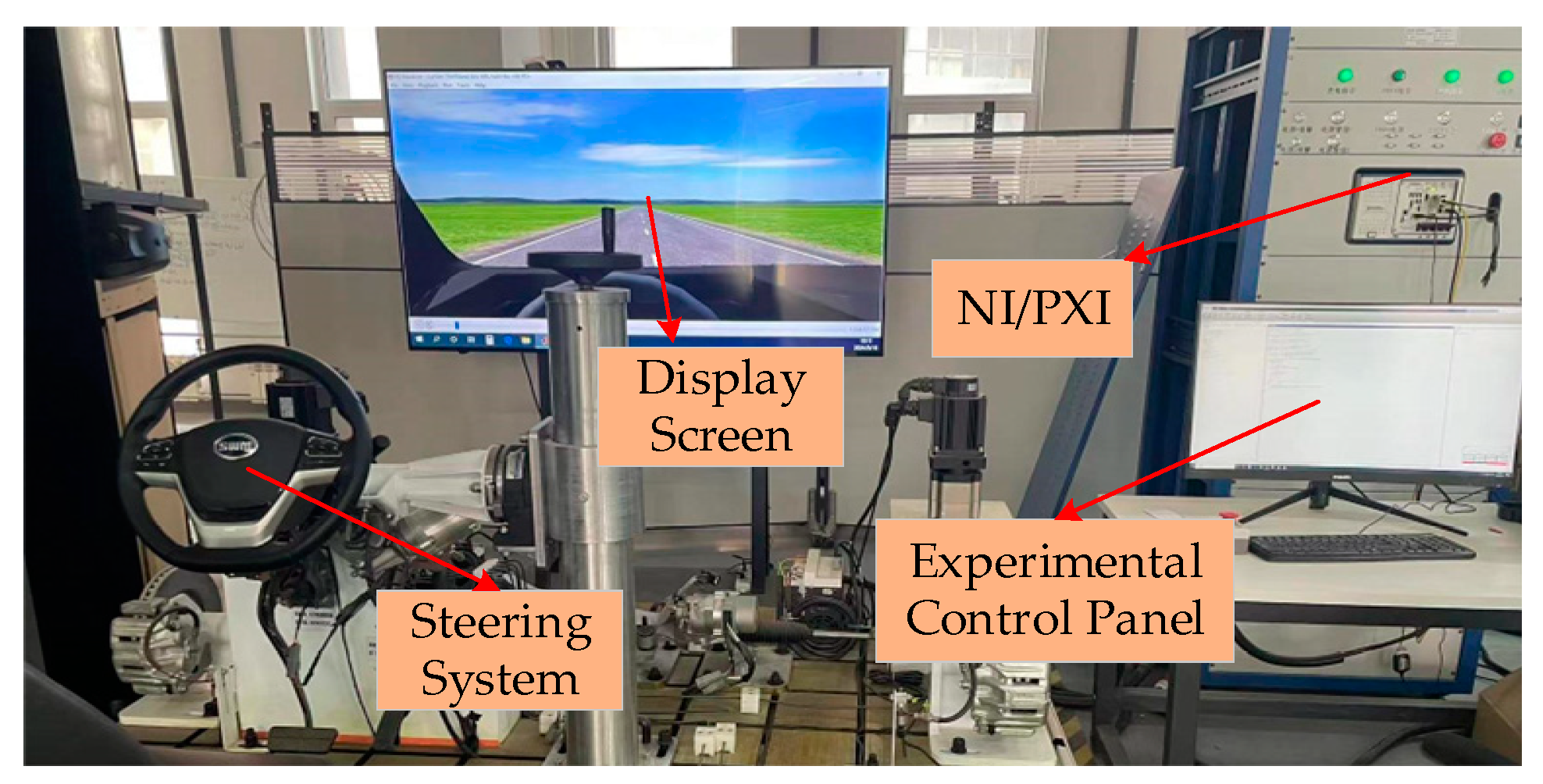
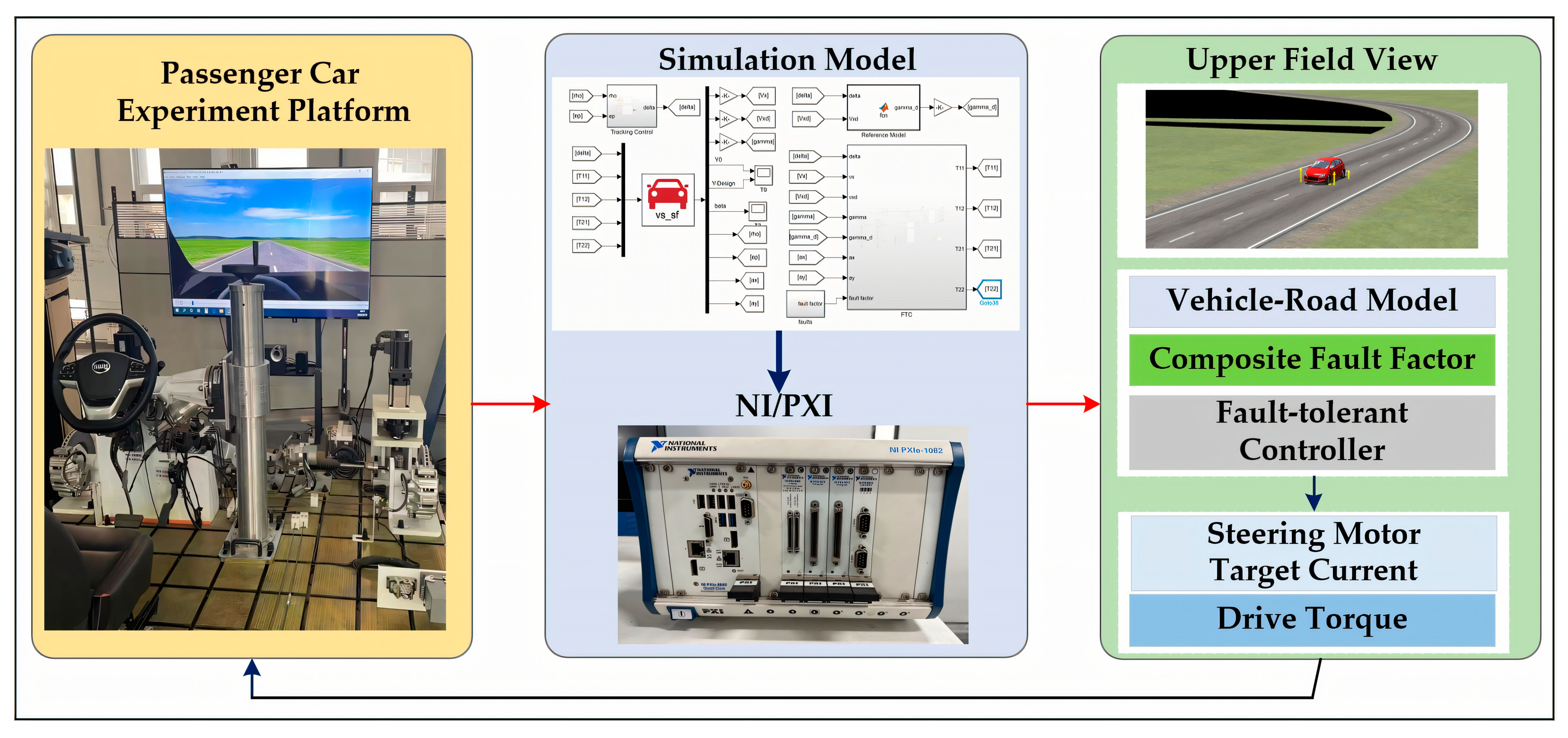
5. Co-Simulation and HIL Experiments

In this paper, the LPV/H∞ output feedback fault-tolerant controller is designed to solve the problem of drive actuator failure while driving and to improve the performance of the vehicle in case of drive actuator failure. To verify the performance of the designed fault-tolerant controller, simulation comparison experiments with the H∞ fault-tolerant controller were conducted in CarSim and Simulink, and experimental verification was carried out in the HIL environment. The parameters required in the experiments are all given by the B-class vehicle model in the CarSim software and can be found in

Table 1. Vehicle dynamics parameters.

Parameter	Value	Units	Parameter	Value	Units
m	1274	kg	$l_r$	1.523	m
Ca	0.3	Null	$h_g$	0.375	m
$C_f$	120,000	N/rad	$d_t$	1.739	m
$C_r$	100,000	N/rad	$R_t$	0.303	m
$l_f$	1.016	m	$I_z$	1523	kg·m2

The relation equation for the rotational inertia $I_z$ in the table is $I_z=m\ast R_z^2$, where $R_z$ is the radius of gyration and the size is 1.093 m.

. In addition, to ensure the fairness of the experiments, the parameters of the vehicles and the experimental environments were the same when the comparison experiments were conducted, except for the different control methods. In the simulation and experimental results, (*) indicates the presence of an actuator fault.

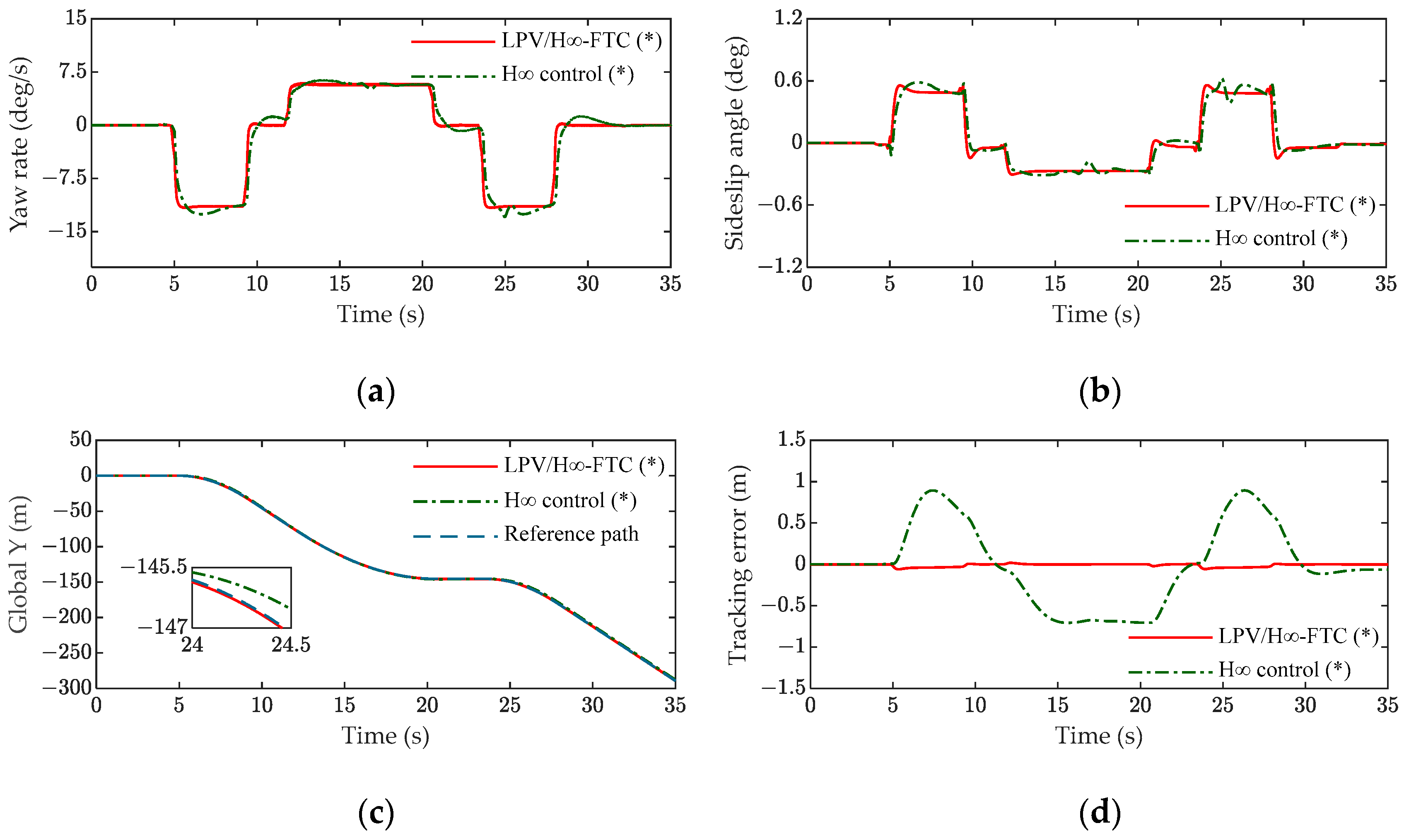
5.1. Analysis of Simulation Results

To verify the performance of the FTC under 4WID electric vehicle path tracking, this section adopts three different path tracking driving environments of a straight line, single shift line, and S-turn to conduct simulation experiments, and analyzes the results accordingly. The vehicle parameters and external environment are the same in the experiments.

Scene A: In the experiment, the vehicle traveled at a speed of 72 km/h in an S-turn with an adhesion coefficient of 0.85; the vehicle’s path is shown in Figure 3c. The fault situation of the actuator was as follows: at 4s, the left front wheel had a stuck fault ${\phi }_{fl}=0$, and at 10 s, the right rear wheel had an additional fault, ${\Delta T}_{rr}=10 \mathrm{N}/\mathrm{m}$. (a) and (b) in Figure 3 are respectively the yaw rate of the vehicle and the side slip angle. When the fault occurred, the vehicle state parameters of the LPV/H∞ controller were relatively stable, while the H∞ controller had large fluctuations when passing the curve. As shown in Figure 3c,d, both controllers had obvious tracking effects, but the maximum tracking error of the LPV/H∞ controller was only 6.59% of that of the H∞ controller (the maximum tracking error can be found in

Table 2. Performance comparison of different control schemes in simulation experiments.

Experimental Scene	Control Strategy	Fault Status	Performance Comparison
			$\mathbf{max}\left(\left|\mathit{\gamma }\right|\right)$	$\mathbf{max}\left(\left|\mathit{\beta }\right|\right)$	$\mathbf{max}\left(\left|\mathit{e}\right|\right)$
S-turn	$\mathit{LPV}/H\infty \text{-}\mathrm{FTC}$	Status 2, 4	12.8166 deg/s	0.5765°	0.0603 m
	$H\infty$ Control	Status 2, 4	14.7888 deg/s	0.6926°	0.9205 m
Change lanes	$\mathit{LPV}/H\infty \text{-}\mathrm{FTC}$	Status 3 4	5.9135 deg/s	0.3150°	0.0471 m
	$H\infty$ Control	Status 3, 4	6.8536 deg/s	0.3585°	0.5239 m
Straight line	$\mathit{LPV}/H\infty \text{-}\mathrm{FTC}$	Status 3	0.0372 deg/s	0.0071°	0.0002 m
	$H\infty$ Control	Status 3	0.3837 deg/s	0.0553°	0.0613 m

), and the tracking effect was better.

Scene B: In the experiment, the vehicle was subjected to lane changing (and a single shift line condition) at a speed of 72 km/h on a road surface with a coefficient of adhesion of 0.85; the driving path is shown in Figure 4c. The actuator failure was as follows: at 3 s, the left front wheel had a failure fault ${\phi }_{fl}=0.5$, and at 5 s, the right rear wheel had a stuck fault ${\phi }_{rr}=0$. (a) and (b) in Figure 4 are the vehicle state parameters, including the yaw rate and side slip angle. When a fault occurred, the state parameters of the LPV/H∞ controller were relatively stable, while the state parameters of the H∞ controller had obvious changes. As shown in Figure 4c,d, the maximum tracking error of the LPV/H∞ controller was 8.99% of that of the H∞ controller, and the tracking error was limited to 0.05. Therefore, the tracking effect of the LPV/H∞ controller was better.

Scene C: In the experiment, the vehicle was driven at a speed of 72 km/h on a straight road with a coefficient of adhesion of 0.85; the driving path is shown in Figure 5c. The actuator failure was as follows: at 3 s, the left front wheel had a failure fault ${\phi }_{fl}=0.6$, and at 10 s, the right rear wheel had a failure fault ${\phi }_{rr}=0.4$. (a) and (b) in Figure 5 are the vehicle state parameters. Combined with Table 2, when a fault occurs, the yaw rate of the LPV/H∞ controller was restricted within 0.005 and the side slip angle was restricted within 0.05. The state parameters were very stable, while the state parameters of the H∞ controller changed significantly. As shown in Figure 5c,d, both controllers had good tracking effects, but the maximum tracking error of the LPV/H∞ controller was only 2.07% that of the H∞ controller, and the tracking performance was better.

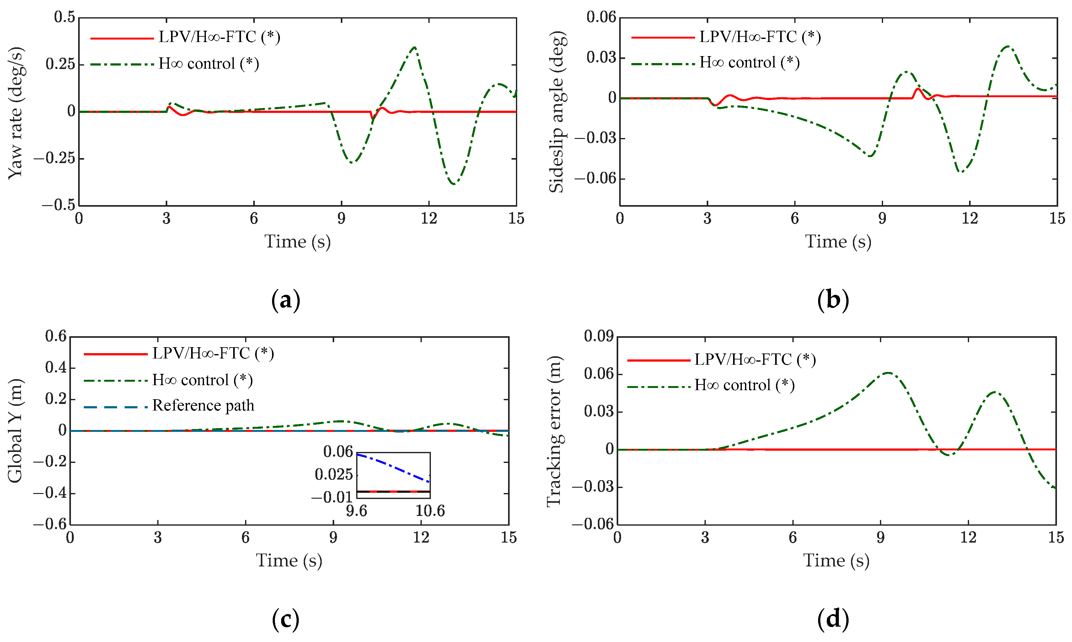
5.2. Analysis of HIL Experiment Results

To verify the real-time performance of the fault-tolerant control strategy, HIL experiments were conducted. The passenger car HIL experimental platform mainly consisted of a steering system, NI/PXI, a display screen, and an experimental control panel, as shown in Figure 6.

Figure 7 shows the specific architecture diagram for realizing the fault-tolerant control hardware-in-the-loop system. The realization process was as follows: first, the designed controller simulation model was embedded into the LabVIEW program, and the NI/PXI sent the calculated front wheel angle to the underlying steering controller according to the real-time calculation of vehicle state information. Secondly, the calculated driving torques of the four driving wheels were sent to the lower layer controller. After the steering system and drive actuators worked, NI/PXI received real-time feedback from the processing pedestal via CAN bus, and then the CarSim in it generated the new vehicle state information to form the closed-loop control. Finally, the vehicle’s trajectory could be observed in real-time through the display screen, and the data curve generated by the data acquisition module could be observed on the experimental control panel.

The HIL experiment in this paper includes two experimental environments: S-turn and change lanes (single shift line). As shown in (c) and (d) in Figure 8, both controllers could maintain a good tracking effect when the vehicle was driving at high speed in curve S. After the fault occurred when the vehicle passed through the curve, the tracking error of the LPV/H∞ controller was controlled within 0.1m, while the H∞ controller produced a large tracking error (the maximum tracking error value can be found in

Table 3. Performance comparison of different control schemes in the HIL experiments.

Experimental Scene	Control Strategy	Fault Status	Performance Comparison
			$\mathbf{max}\left(\left|\mathit{\gamma }\right|\right)$	$\mathbf{max}\left(\left|\mathit{\beta }\right|\right)$	$\mathbf{max}\left(\left|\mathit{e}\right|\right)$
S-turn	$\mathit{LPV}/H\infty \text{-}\mathrm{FTC}$	Status 2, 4	11.6386 deg/s	0.5594°	0.0589 m
	$H\infty$ Control	Status 2, 4	12.9392 deg/s	0.6256°	0.8937 m
Change lanes	$\mathit{LPV}/H\infty \text{-}\mathrm{FTC}$	Status 3 4	6.9521 deg/s	0.2748°	0.1663 m
	$H\infty$ Control	Status 3 4	9.5229 deg/s	0.3414°	0.5013 m

Status 2: additional failure, Status 3: failure fault, Status 4: stuck fault.

). Figure 8a,b show the yaw speed and side yaw angle of the vehicle. Compared with the H∞ controller, the maximum yaw speed and the maximum side yaw angle of the LPV/H∞ controller were reduced by 10.05% and 10.58%. As shown in Figure 9c,d, in the process of a high-speed lane change, the trajectory offset of the LPV/H∞ controller was controlled within 0.17 m, while the maximum trajectory offset of the H∞ controller was 0.5 m. As shown in Figure 9a,b, compared with the H∞ controller, the maximum yaw rate of the LPV/H∞ controller was reduced by 27.00%, and that of the LPV/H∞ controller was reduced by 19.51%. In general, both controllers could maintain the tracking effect after the failure occurred, and the LPV/H∞ controller performed better.

6. Conclusions

In this paper, an output feedback-based LPV/H∞ fault-tolerant controller is proposed for the faulty 4WID electric vehicles drive actuator to improve the driving stability and safety of the vehicle. Firstly, a generalized fault model of the drive system is established, the most common fault types of the drive motor are analyzed, and the comprehensive fault factors of both sides of the vehicle are designed from this, to obtain the LPV model containing the drive actuator faults; secondly, a weighting function is introduced and an LPV/H∞ output feedback fault-tolerant controller is designed, which is solved by solving the matrix inequality for the controller; Finally, the effectiveness of the controller designed in this paper was verified through simulation and hardware-in-the-loop experiments, which proved that the controller can redistribute the driving torque when the drive actuator fails, thus improving the driving stability and safety of the vehicle. In future research work, we will continue to explore the impact of drive actuator failure on other aspects of the vehicle, which will help us to more accurately assess and deal with drive actuator failure, thus improving the overall stability and driving safety of the vehicle.

References

1. Barari, A.; Afshari, S.S.; Liang, X. Coordinated control for path-following of an autonomous four in-wheel motor drive electric vehicle. Proc. Inst. Mech. Eng. Part C J. Mech. Eng. Sci. 2022, 236, 6335–6346. [Google Scholar] [CrossRef] [PubMed]
2. Xie, Y.; Li, C.; Jing, H.; An, W.; Qin, J. Integrated control for path tracking and stability based on the model predictive control for four-wheel independently driven electric vehicles. Machines 2022, 10, 859. [Google Scholar] [CrossRef]
3. Li, Z.; Jiao, X.; Zhang, T. Robust H∞ Output Feedback Trajectory Tracking Control for Steer-by-Wire Four-Wheel Independent Actuated Electric Vehicles. World Electr. Veh. J. 2023, 14, 147. [Google Scholar] [CrossRef]
4. Baldini, A.; Felicetti, R.; Freddi, A.; Longhi, S.; Monteriù, A. Actuator fault-tolerant control architecture for multirotor vehicles in presence of disturbances. J. Intell. Robot. Syst. 2020, 99, 859–874. [Google Scholar] [CrossRef]
5. You, Z. Fault Tolerant Control Method of Power System of Tram Based on PLC. Jordan J. Mech. Ind. Eng. 2021, 15, 133–142. [Google Scholar]
6. Zhu, S.; Li, H.; Wang, G.; Kuang, C.; Chen, H.; Gao, J.; Xie, W. Research on Fault-Tolerant Control of Distributed-Drive Electric Vehicles Based on Fuzzy Fault Diagnosis. Actuators 2023, 12, 246. [Google Scholar] [CrossRef]
7. Zhang, B.; Lu, S. Fault-tolerant control for four-wheel independent actuated electric vehicle using feedback linearization and cooperative game theory. Control Eng. Pract. 2020, 101, 104510. [Google Scholar] [CrossRef]
8. Liu, Y.; Zong, C.; Zhang, D.; Zheng, H.; Han, X.; Sun, M. Fault-tolerant control approach based on constraint control allocation for 4WIS/4WID vehicles. Proc. Inst. Mech. Eng. Part D J. Automob. Eng. 2021, 235, 2281–2295. [Google Scholar] [CrossRef]
9. Wu, C.; Sehab, R.; Akrad, A.; Morel, C. Fault diagnosis methods and Fault tolerant control strategies for the electric vehicle powertrains. Energies 2022, 15, 4840. [Google Scholar] [CrossRef]
10. Li, H.; Zhang, N.; Wu, G.; Li, Z.; Ding, H.; Jiang, C. Active Fault-Tolerant Control of a Four-Wheel Independent Steering System Based on the Multi-Agent Approach. Electronics 2024, 13, 748. [Google Scholar] [CrossRef]
11. Hu, C.; Wei, X.; Ren, Y. Passive fault-tolerant control based on weighted LPV tube-MPC for air-breathing hypersonic vehicles. Int. J. Control Autom. Syst. 2019, 17, 1957–1970. [Google Scholar] [CrossRef]
12. El-Bakkouri, J.; Ouadi, H.; Giri, F.; Saad, A. Optimal control for anti-lock braking system: Output feedback adaptive controller design and processor in the loop validation test. Proc. Inst. Mech. Eng. Part D J. Automob. Eng. 2022, 237, 3465–3477. [Google Scholar] [CrossRef]
13. Aljarbouh, A.; Fayaz, M.; Qureshi, M.S.; Boujoudar, Y. Hybrid sliding mode control of full-car semi-active suspension systems. Symmetry 2021, 13, 2442. [Google Scholar] [CrossRef]
14. Girovský, P.; Žilková, J.; Kaňuch, J. Optimization of vehicle braking distance using a fuzzy controller. Energies 2020, 13, 3022. [Google Scholar] [CrossRef]
15. Liang, J.; Tian, Q.; Feng, J.; Pi, D.; Yin, G. A polytopic model-based robust predictive control scheme for path tracking of autonomous vehicles. IEEE Trans. Intell. Veh. 2023, 9, 3928–3939. [Google Scholar] [CrossRef]
16. He, X.; Huang, W.; Lv, C. Trustworthy autonomous driving via defense-aware robust reinforcement learning against worst-case observational perturbations. Transp. Res. Part C Emerg. Technol. 2024, 163, 104632. [Google Scholar] [CrossRef]
17. He, X.; Huang, W.; Lv, C. Toward trustworthy decision-making for autonomous vehicles: A robust reinforcement learning approach with safety guarantees. Engineering 2024, 33, 77–89. [Google Scholar] [CrossRef]
18. Zhou, Z.; Zhu, J.; Li, Y. Robust control of vehicle multi-target adaptive cruise based on model prediction. Cogn. Comput. Syst. 2020, 2, 254–261. [Google Scholar] [CrossRef]
19. Kou, F.; Chen, C.; Xiao, W.; Hu, K. Study on Adaptive Sliding Mode Fault-tolerant Control of 1/4 Vehicle Electromagnetic Suspension. J. Phys.: Conf. Ser. 2023, 2528, 012025. [Google Scholar]
20. Zhang, B.; Lu, S.; Zhao, L.; Xiao, K. Fault-tolerant control based on 2D game for independent driving electric vehicle suffering actuator failures. Proc. Inst. Mech. Eng. Part D J. Automob. Eng. 2020, 234, 3011–3025. [Google Scholar] [CrossRef]
21. Yang, K.; Tang, X.; Qin, Y.; Huang, Y.; Wang, H.; Pu, H. Comparative study of trajectory tracking control for automated vehicles via model predictive control and robust H-infinity state feedback control. Chin. J. Mech. Eng. 2021, 34, 1–14. [Google Scholar] [CrossRef]
22. Liang, J.; Wang, F.; Feng, J.; Zhao, M.; Fang, R.; Pi, D.; Yin, G. A Hierarchical Control of Independently Driven Electric Vehicles Considering Handling Stability and Energy Conservation. IEEE Trans. Intell. Veh. 2023, 9, 738–751. [Google Scholar] [CrossRef]
23. Li, P.; Nguyen, A.T.; Du, H.; Wang, Y.; Zhang, H. Polytopic LPV approaches for intelligent automotive systems: State of the art and future challenges. Mech. Syst. Signal Process. 2021, 161, 107931. [Google Scholar] [CrossRef]
24. Long, Y.; Feng, J.; Zhang, R.; Wei, T. H∞ Robust Fault-Tolerant Control for Lateral Stability of Four-wheel independent driving EV. Mech. Sci. Technol. Aerosp. Eng. 2023, 42, 92–98. [Google Scholar]
25. Nguyen, M.Q.; Sename, O.; Dugard, L. An LPV fault tolerant control for semi-active suspension-scheduled by fault estimation. IFAC-PapersOnLine 2015, 48, 42–47. [Google Scholar] [CrossRef]
26. Tayari, R.; Ben Brahim, A.; Ben Hmida, F.; Sallami, A. Active fault tolerant control design for lpv systems with simultaneous actuator and sensor faults. Math. Probl. Eng. 2019, 2019, 1–14. [Google Scholar] [CrossRef]
27. Wang, H.; Cui, W.; Lin, S.; Tan, D.; Chen, W. Stability control of in-wheel motor drive vehicle with motor fault. Proc. Inst. Mech. Eng. Part D J. Automob. Eng. 2019, 233, 3147–3164. [Google Scholar] [CrossRef]
28. Zhang, L.; Yu, W.; Wang, Z.; Ding, X. Fault tolerant control based on multi-methods switching for four-wheel-independently-actuated electric vehicles. J. Mech. Eng. 2020, 56, 227–239. [Google Scholar]
29. Lee, K.; Lee, M. Fault-tolerant stability control for independent four-wheel drive electric vehicle under actuator fault conditions. IEEE Access 2020, 8, 91368–91378. [Google Scholar] [CrossRef]
30. Luo, Y.; Cao, K.; Xie, L.; Li, K. Coordinated fault tolerant control of over-actuated electric vehicles based on optimal tyre force distribution. Int. J. Veh. Des. 2017, 75, 47–74. [Google Scholar] [CrossRef]
31. Luo, Y.; Hu, Y.; Jiang, F.; Chen, R.; Wang, Y. Active fault-tolerant control based on multiple input multiple output-model free adaptive control for four wheel independently driven electric vehicle drive system. Appl. Sci. 2019, 9, 276. [Google Scholar] [CrossRef]
32. Yao, Y.; Li, E.; Peng, C. Research on the Distribution Strategy of Longitudinal Driving Force of Vehicle Driven by 8× 8 In-wheel Motors. J. Phys. Conf. Ser. 2022, 2181, 012017. [Google Scholar] [CrossRef]
33. Huang, X.; Zha, Y.; Lv, X.; Quan, X. Torque Fault-Tolerant Hierarchical Control of 4WID Electric Vehicles Based on Improved MPC and SMC. IEEE Access 2023, 11, 132718–132734. [Google Scholar] [CrossRef]
34. Zhang, L.; Wang, Z.; Ding, X.; Li, S.; Wang, Z. Fault-tolerant control for intelligent electrified vehicles against front wheel steering angle sensor faults during trajectory tracking. IEEE Access 2021, 9, 65174–65186. [Google Scholar] [CrossRef]
35. Liu, X.; Pang, H.; Shang, Y.; Wu, W. Optimal design of fault-tolerant controller for an electric power steering system with sensor failures using genetic algorithm. Shock Vib. 2018, 2018, 1801589. [Google Scholar] [CrossRef]
36. Khaneghah, M.Z.; Alzayed, M.; Chaoui, H. Fault detection and diagnosis of the electric motor drive and battery system of electric vehicles. Machines 2023, 11, 713. [Google Scholar] [CrossRef]
37. Şimşir, M.; Bayır, R.; Uyaroğlu, Y. Real-time monitoring and fault diagnosis of a low power hub motor using feedforward neural network. Comput. Intell. Neurosci. 2015, 2016, 36. [Google Scholar] [CrossRef] [PubMed]
38. Chen, W.; Liang, X.; Wang, Q.; Zhao, L.; Wang, X. Extension coordinated control of four wheel independent drive electric vehicles by AFS and DYC. Control Eng. Pract. 2020, 101, 104504. [Google Scholar] [CrossRef]
39. Liang, J.; Feng, J.; Fang, Z.; Lu, Y.; Yin, G.; Mao, X.; Wu, J.; Wang, F. An energy-oriented torque-vector control framework for distributed drive electric vehicles. IEEE Trans. Transp. Electrif. 2023, 9, 4014–4031. [Google Scholar] [CrossRef]
40. Nah, J.; Yim, S. Vehicle stability control with four-wheel independent braking, drive and steering on in-wheel motor-driven electric vehicles. Electronics 2020, 9, 1934. [Google Scholar] [CrossRef]
41. He, X.; Liu, Y.; Yang, K.; Wu, J.; Ji, X. Robust coordination control of AFS and ARS for autonomous vehicle path tracking and stability. In Proceedings of the 2018 IEEE International Conference on Mechatronics and Automation, Changchun, China, 5–8 August 2018; pp. 924–929. [Google Scholar]
42. Lin, J.; Zou, T.; Su, L.; Zhang, F.; Zhang, Y. Optimal Coordinated Control of Active Front Steering and Direct Yaw Moment for Distributed Drive Electric Bus. Machines 2023, 11, 640. [Google Scholar] [CrossRef]
43. Apkarian, P.; Gahinet, P.; Becker, G. Self-scheduled H∞ control of linear parameter-varying systems: A design example. Automatica 1995, 31, 1251–1261. [Google Scholar] [CrossRef]
44. Scherer, C.; Gahinet, P.; Chilali, M. Multiobjective output-feedback control via LMI optimization. IEEE Trans. Autom. Control 1997, 42, 896–911. [Google Scholar] [CrossRef]
Figure 1. Simplified car modeling.
Machines 12 00450 g001
Figure 2. Fault tolerant control strategy scheme.
Machines 12 00450 g002
Figure 3. Simulation results. (a) Yaw rate, (b) sideslip angle, (c) vehicle tracks, (d) tracking error.
Machines 12 00450 g003
Figure 4. Simulation results. (a) Yaw rate, (b) sideslip angle, (c) vehicle tracks, (d) tracking error.
Machines 12 00450 g004
Figure 5. Simulation results. (a) Yaw rate, (b) sideslip angle, (c) vehicle tracks, (d) tracking error.
Machines 12 00450 g005
Figure 6. Hardware-in-the-loop experimental platform for passenger cars.
Machines 12 00450 g006
Figure 7. Fault-tolerant control HIL test framework for passenger vehicles.
Machines 12 00450 g007
Figure 8. Experimental results. (a) Yaw rate, (b) sideslip angle, (c) vehicle tracks, (d) tracking error.
Machines 12 00450 g008
Figure 9. Experimental results. (a) Yaw rate, (b) sideslip angle, (c) vehicle tracks, (d) tracking error.
Machines 12 00450 g009