
A Review of the Intelligent Condition Monitoring of Rolling Element Bearings


Abstract
1. Introduction
- What are the main approaches for sensing and signal processing to extract features for bearing faults? How can signal integrity be enhanced and uncertainty reduced?
- What kinds of information fusion techniques are being used to improve the reliability of bearing fault diagnosis?
- How are intelligent algorithms driving rapid advancements in bearing monitoring and diagnosis? What are the frontier intelligent techniques and the challenges associated with them?
2. Fundamentals and Sensing Strategies
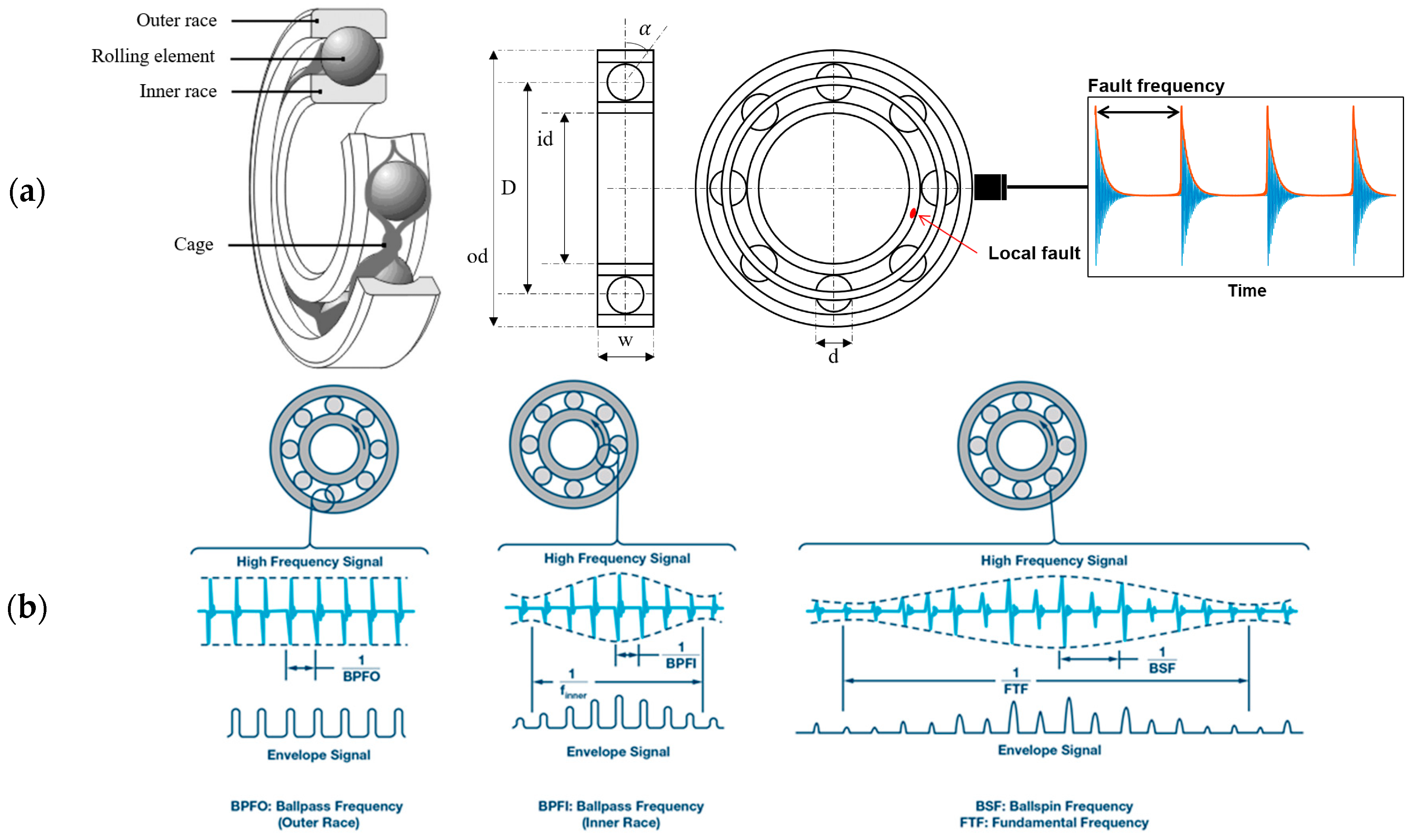
2.1. Defect Frequencies of Rolling Element Bearings
2.2. Condition Monitoring Approaches
2.2.1. Vibration-Based Monitoring
2.2.2. Acoustic Emission-Based Monitoring
2.2.3. Thermal-Based Monitoring
2.2.4. Other Approaches
2.3. Influence of Sensor Integrity
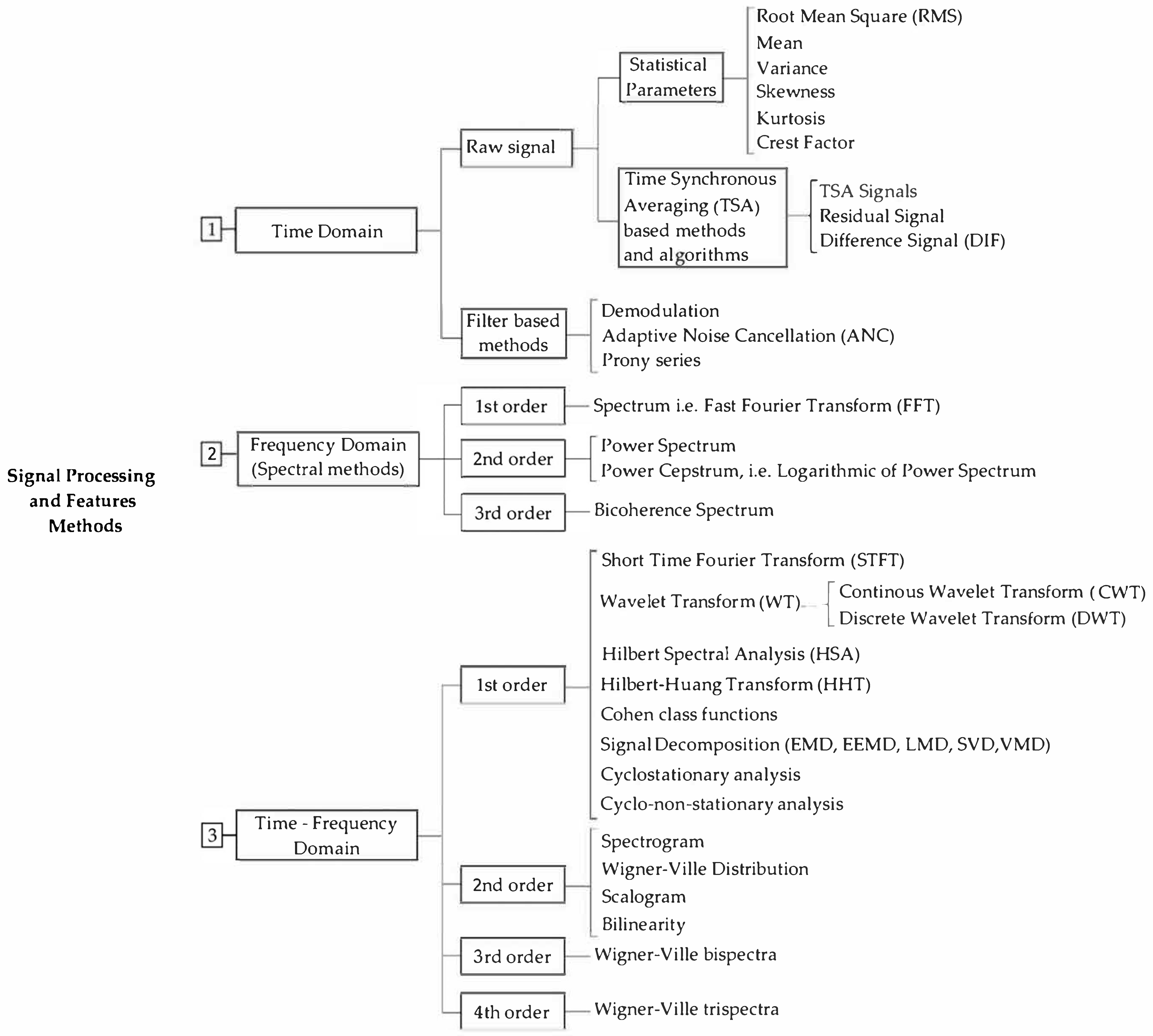
3. Signal Processing and Feature Extraction Techniques
3.1. Time Domain Methods
3.2. Frequency Domain Methods
3.3. Time–Frequency Domain Methods
4. Information Fusion
4.1. Data-Level Fusion
4.2. Feature-Level Fusion
4.3. Decision-Level Fusion
4.4. Multi-Level Fusion
5. Intelligent Algorithms and Applications
5.1. Machine Learning and Deep-Learning Approaches
5.2. Metaheuristic Optimisation Techniques
5.3. Deep-Learning Approaches
6. Conclusions and Future Perspectives
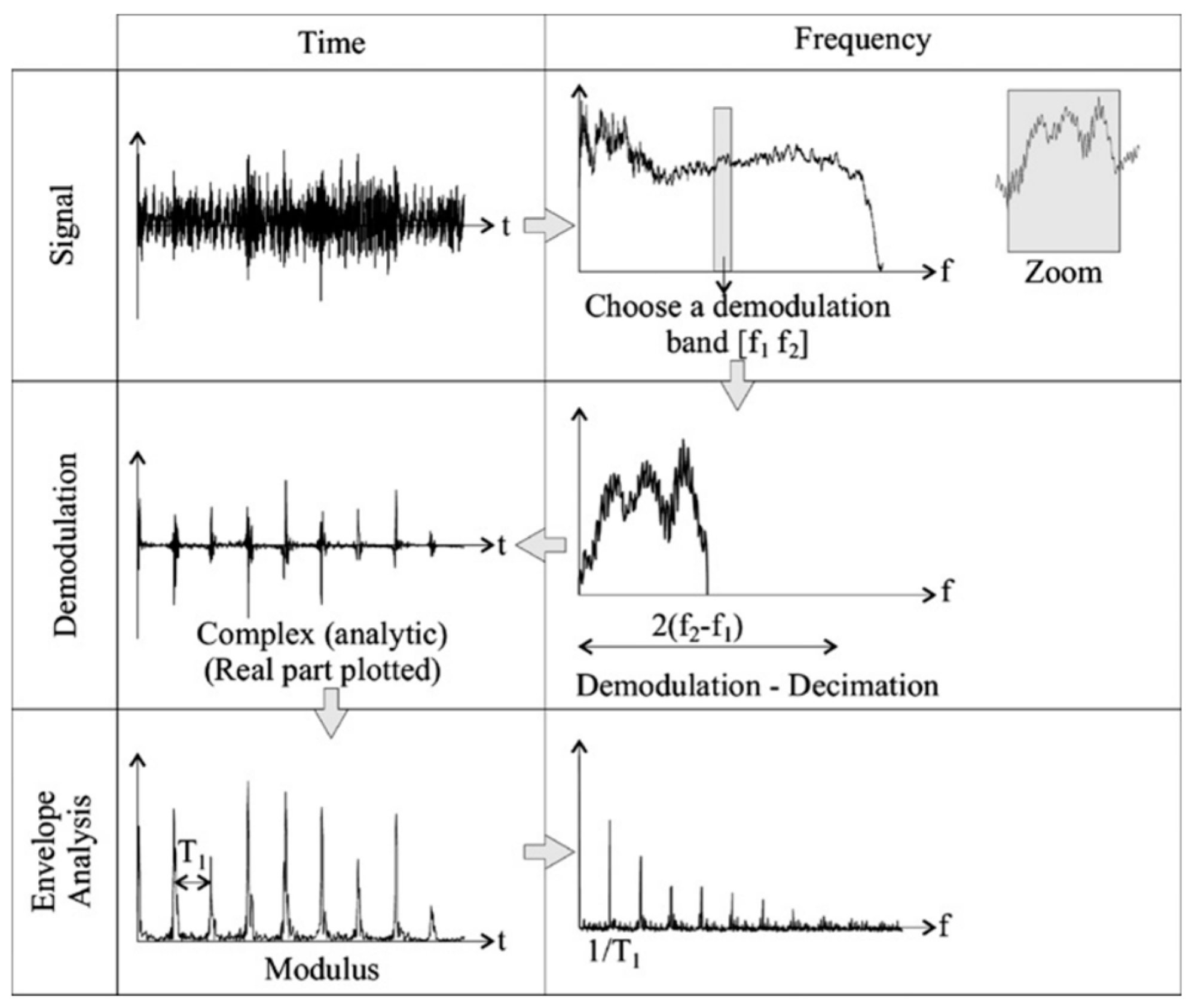
- The envelope spectrum has proven to be an efficient benchmarking technique in the defect detection and diagnosis of bearings. The selection of an optimal frequency band for demodulation is crucial for this. While various techniques have been explored, many are time-consuming or require specialised expertise. New envelope spectrum approaches, such as the log-envelope and product envelope spectrum, have shown an improved performance. Further research leveraging metaheuristic optimisation and deep learning for automatic demodulation band selection and multi-band integration could enhance efficiency in this area.
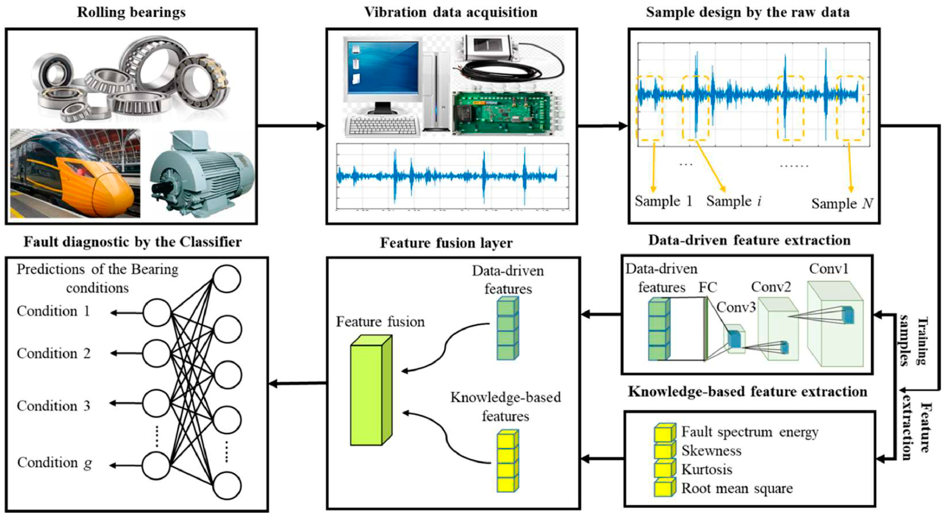
- AI-based fault diagnosis techniques have become prominent due to their rapid development in the ability to significantly enhance the accuracy, efficiency, and reliability. Machine-learning classifiers are often used for diagnostic tasks due to their ability to achieve high accuracy without extensive domain knowledge. The classifier can be trained well for fault identification through the extraction of relevant features pertaining to the bearing health condition from historic data. It would be more practical for a signal integrity assessment technique to work on a variety of issues so it can be used as a standard preprocessing step to fault diagnosis. Research in the area will benefit from the development of a classification model that accurately captures the nonrigid nature of the decision boundary of signals to efficiently segregate anomalies.
- Multi-sensor monitoring systems were found to be advantageous as they increased the general reliability of fault detection and diagnosis. The use of heterogeneous sensors in conjunction can also aid in further increasing the reliability. While information fusion of different sensors has been achieved on different levels, it is most common for decision-level fusion to take place. However, conflicting results in sensor diagnoses can occur due to misclassification in learning models or sensor integrity issues, highlighting the need for further research to address these challenges.
- There are significant opportunities to employ innovative deep-learning technologies to address challenges in bearing fault diagnosis, such as the time-varying conditions, unlabelled and imbalanced data, complex fault patterns, and real-time detection for the fault types and locations. It is important to design the deep learning-based diagnosis systems that are lightweight, computationally efficient, and fast in execution. In addition, a deep understanding of the mechanics and physics of fault-related features is vital for the success of these monitoring systems.
Author Contributions
Funding
Data Availability Statement
Conflicts of Interest
References
- Cong, F.; Chen, J.; Dong, G.; Pecht, M. Vibration model of rolling element bearings in a rotor-bearing system for fault diagnosis. J. Sound Vib. 2013, 332, 2081–2097. [Google Scholar] [CrossRef]
- Ali, J.B.; Fnaiech, N.; Saidi, L.; Chebel-Morello, B.; Fnaiech, F. Application of empirical mode decomposition and artificial neural network for automatic bearing fault diagnosis based on vibration signals. Appl. Acoust. 2015, 89, 16–27. [Google Scholar] [CrossRef]
- Wang, T.; Liang, M.; Li, J.; Cheng, W. Rolling element bearing fault diagnosis via fault characteristic order (FCO) analysis. Mech. Syst. Signal Process. 2014, 45, 139–153. [Google Scholar] [CrossRef]
- Randall, R.B.; Monitoring, V.-B.C. Aerospace and Automotive Applications, 1st ed.; John Wiley & Sons: Hoboken, NJ, USA, 2011. [Google Scholar]
- Mollasalehi, E. Data-Driven and Model-Based Bearing Fault Analysis—Wind Turbine Application. Ph.D. Thesis, University of Calgary, Calgary, AB, Canada, 2017. [Google Scholar]
- Khaleghi, B.; Khamis, A.; Karray, F.O.; Razavi, S.N. Multisensor data fusion: A review of the state-of-the-art. Inf. Fusion 2013, 14, 28–44. [Google Scholar] [CrossRef]
- Duan, Z.; Wu, T.; Guo, S.; Shao, T.; Malekian, R.; Li, Z. Development and trend of condition monitoring and fault diagnosis of multi-sensors information fusion for rolling bearings: A review. Int. J. Adv. Manuf. Technol. 2018, 96, 803–819. [Google Scholar] [CrossRef]
- Liu, R.; Yang, B.; Zio, E.; Chen, X. Artificial intelligence for fault diagnosis of rotating machinery: A review. Mech. Syst. Signal Process. 2018, 108, 33–47. [Google Scholar] [CrossRef]
- Gryllias, K.C.; Antoniadis, I.A. A Support Vector Machine approach based on physical model training for rolling element bearing fault detection in industrial environments. Eng. Appl. Artif. Intell. 2012, 25, 326–344. [Google Scholar] [CrossRef]
- Caesarendra, W.; Tjahjowidodo, T. A review of feature extraction methods in vibration-based condition monitoring and its application for degradation trend estimation of low-speed slew bearing. Machines 2017, 5, 21. [Google Scholar] [CrossRef]
- Moshrefzadeh, A. Condition monitoring and intelligent diagnosis of rolling element bearings under constant/variable load and speed conditions. Mech. Syst. Signal Process. 2021, 149, 107153. [Google Scholar] [CrossRef]
- Malla, C.; Panigrahi, I. Review of Condition Monitoring of Rolling Element Bearing Using Vibration Analysis and Other Techniques. J. Vib. Eng. Technol. 2019, 7, 407–414. [Google Scholar] [CrossRef]
- Alshorman, O.; Irfan, M.; Saad, N.; Zhen, D.; Haider, N.; Glowacz, A.; Alshorman, A. A Review of Artificial Intelligence Methods for Condition Monitoring and Fault Diagnosis of Rolling Element Bearings for Induction Motor. Shock Vib. 2020, 2020, 8843759. [Google Scholar] [CrossRef]
- Boudinar, A.H.; Benouzza, N.; Bendiabdellah, A.; Khodja, M. Induction Motor Bearing Fault Analysis Using a Root-MUSIC Method. IEEE Trans. Ind. Appl. 2016, 52, 3851–3860. [Google Scholar] [CrossRef]
- Kim, S.; An, D.; Choi, J.H. Diagnostics 101: A tutorial for fault diagnostics of rolling element bearing using envelope analysis in MATLAB. Appl. Sci. 2020, 10, 7302. [Google Scholar] [CrossRef]
- Singh, S.; Howard, C.Q.; Hansen, C.H. An extensive review of vibration modelling of rolling element bearings with localised and extended defects. J. Sound Vib. 2015, 357, 300–330. [Google Scholar] [CrossRef]
- Sopcik, P.; O’sullivan, D. How Sensor Performance Enables Condition-Based Monitoring Solutions. Analog Dialogue 2019, 53, 1–5. [Google Scholar]
- Smith, W.A.; Randall, R.B. Rolling element bearing diagnostics using the Case Western Reserve University data: A benchmark study. Mech. Syst. Signal Process. 2015, 64–65, 100–131. [Google Scholar] [CrossRef]
- Randall, R.B.; Antoni, J. Rolling element bearing diagnostics-A tutorial. Mech. Syst. Signal Process. 2011, 25, 485–520. [Google Scholar] [CrossRef]
- Jablonski, A. Condition Monitoring Algorithms in MATLAB®; Springer International Publishing: Cham, Switzerland, 2021. [Google Scholar] [CrossRef]
- Hong, H.; Liang, M. Fault severity assessment for rolling element bearings using the Lempel–Ziv complexity and continuous wavelet transform. J. Sound Vib. 2009, 320, 452–468. [Google Scholar] [CrossRef]
- Suh, S.; Lukowicz, P.; Lee, Y.O. Generalized multiscale feature extraction for remaining useful life prediction of bearings with generative adversarial networks. Knowl. Based Syst. 2022, 237, 107866. [Google Scholar] [CrossRef]
- Randall, R.B.; Smith, W.A. Detection of faulty accelerometer mounting from response measurements. J. Sound Vib. 2020, 477, 115318. [Google Scholar] [CrossRef]
- Al-Ghamd, A.M.; Mba, D. A comparative experimental study on the use of acoustic emission and vibration analysis for bearing defect identification and estimation of defect size. Mech. Syst. Signal Process. 2006, 20, 1537–1571. [Google Scholar] [CrossRef]
- Guo, B.; Song, S.; Ghalambor, A.; Lin, T.R. Offshore Pipelines: Design, Installation, and Maintenance, 2nd ed. Gulf Professional Publishing: Waltham, MA, USA, 2014; 257–297ISBN 978-0-12-397949-0.
- Choudhury, A.; Tandon, N. Application of acoustic emission technique for the detection of defects in rolling element bearings. Tribol. Int. 2000, 33, 39–45. [Google Scholar] [CrossRef]
- Elforjani, M.; Mba, D. Accelerated natural fault diagnosis in slow speed bearings with Acoustic Emission. Eng. Fract. Mech. 2010, 77, 112–127. [Google Scholar] [CrossRef]
- Caesarendra, W.; Kosasih, B.; Tieu, A.K.; Zhu, H.; Moodie, C.A.S.; Zhu, Q. Acoustic emission-based condition monitoring methods: Review and application for low speed slew bearing. Mech. Syst. Signal Process. 2016, 72–73, 134–159. [Google Scholar] [CrossRef]
- Van Hecke, B.; Yoon, J.; He, D. Low speed bearing fault diagnosis using acoustic emission sensors. Appl. Acoust. 2016, 105, 35–44. [Google Scholar] [CrossRef]
- Liu, C.; Wu, X.; Mao, J.; Liu, X. Acoustic emission signal processing for rolling bearing running state assessment using compressive sensing. Mech. Syst. Signal Process. 2017, 91, 395–406. [Google Scholar] [CrossRef]
- Tandon, N.; Parey, A. Condition Monitoring of Rotary Machines. Cond. Monit. Control Intell. Manuf. 2006, 1, 109–136. [Google Scholar] [CrossRef]
- Younus, A.M.D.; Yang, B.S. Intelligent fault diagnosis of rotating machinery using infrared thermal image. Expert Syst. Appl. 2012, 39, 2082–2091. [Google Scholar] [CrossRef]
- Janssens, O.; Schulz, R.; Slavkovikj, V.; Stockman, K.; Loccufier, M.; Van De Walle, R.; Van Hoecke, S. Thermal image based fault diagnosis for rotating machinery. Infrared Phys. Technol. 2015, 73, 78–87. [Google Scholar] [CrossRef]
- Liu, Z.; Wang, J.; Duan, L.; Shi, T.; Fu, Q. Infrared Image Combined with CNN Based Fault Diagnosis for Rotating Machinery. In Proceedings of the 2017 International Conference on Sensing, Diagnostics, Prognostics, and Control (SDPC), Shanghai, China, 16–18 August 2017; pp. 137–142. [Google Scholar] [CrossRef]
- Mehta, A.; Goyal, D.; Choudhary, A.; Pabla, B.S.; Belghith, S. Machine Learning-Based Fault Diagnosis of Self-Aligning Bearings for Rotating Machinery Using Infrared Thermography. Math. Probl. Eng. 2021, 2021, 9947300. [Google Scholar] [CrossRef]
- Wu, T.; Wu, H.; Du, Y.; Peng, Z. Progress and trend of sensor technology for on-line oil monitoring. Sci. China Technol. Sci. 2013, 56, 2914–2926. [Google Scholar] [CrossRef]
- Wang, S.Y.; Yang, D.X.; Hu, H.F. Evaluation for bearing wear states based on online oil multi-parameters monitoring. Sensors 2018, 18, 1111. [Google Scholar] [CrossRef] [PubMed]
- Kim, Y.H.; Tan, A.C.C.; Mathew, J.; Yang, B.S. Condition monitoring of low speed bearings: A comparative study of the ultrasound technique versus vibration measurements. In Engineering Asset Management; Springer: London, UK, 2006; pp. 182–191. [Google Scholar] [CrossRef]
- Lineham, J. Ultrasonic probes for inspecting bearings. World Pumps 2008, 2008, 34–36. [Google Scholar] [CrossRef]
- Zarei, J.; Poshtan, J. Bearing fault detection using wavelet packet transform of induction motor stator current. Tribol. Int. 2007, 40, 763–769. [Google Scholar] [CrossRef]
- Park, J.; Kim, S.; Choi, J.H.; Lee, S.H. Frequency energy shift method for bearing fault prognosis using microphone sensor. Mech. Syst. Signal Process. 2021, 147, 107068. [Google Scholar] [CrossRef]
- Martin, G.; Becker, F.M.; Kirchner, E. A novel method for diagnosing rolling bearing surface damage by electric impedance analysis. Tribol. Int. 2022, 170, 107503. [Google Scholar] [CrossRef]
- Becker-Dombrowsky, F.M.; Koplin, Q.S.; Kirchner, E. Individual Feature Selection of Rolling Bearing Impedance Signals for Early Failure Detection. Lubricants 2023, 11, 304. [Google Scholar] [CrossRef]
- Samanta, B.; Al-Balushi, K.R. Artificial neural network based fault diagnostics of rolling element bearings using time-domain features. Mech. Syst. Signal Process. 2003, 17, 317–328. [Google Scholar] [CrossRef]
- Girondin, V.; Loudahi, M.; Morel, H.; Pekpe, K.M.; Cassar, J. Vibration-based fault detection of accelerometers in helicopters. IFAC Proc. Vol. 2012, 45, 720–725. [Google Scholar] [CrossRef]
- Abboud, D.; Elbadaoui, M.; Becquerelle, S.; Lalmi, M. Detection of Sensor Detachment in Aircraft Engines Using Vibration Signals. In Proceedings of the 10th International Conference on Rotor Dynamics—IFToMM; Springer: Cham, Switzerland, 2019; pp. 351–365. [Google Scholar]
- Song, L.; Wang, H.; Chen, P. Automatic signal quality check and equipment condition surveillance based on trivalent logic diagnosis theory. Meas. J. Int. Meas. Confed. 2019, 136, 173–184. [Google Scholar] [CrossRef]
- Kannan, V.; Dao, D.V.; Li, H. Detection of Signal Integrity Issues in Vibration Monitoring Using One-Class Support Vector Machine. J. Vib. Eng. Technol. 2024. [Google Scholar] [CrossRef]
- Bagavathiappan, S.; Lahiri, B.B.; Saravanan, T.; Philip, J.; Jayakumar, T. Infrared thermography for condition monitoring—A review. Infrared Phys. Technol. 2013, 60, 35–55. [Google Scholar] [CrossRef]
- Tiboni, M.; Remino, C.; Bussola, R.; Amici, C. A Review on Vibration-Based Condition Monitoring of Rotating Machinery. Appl. Sci. 2022, 12, 972. [Google Scholar] [CrossRef]
- Shen, Z.; He, Z.; Chen, X.; Sun, C.; Liu, Z. A monotonic degradation assessment index of rolling bearings using fuzzy support vector data description and running time. Sensors 2012, 12, 10109–10135. [Google Scholar] [CrossRef] [PubMed]
- Tom, K.F. A Primer on Vibrational Ball Bearing Feature Generation for Prognostics and Diagnostics Algorithms. ARL-TR-7230, March 2015. Available online: https://apps.dtic.mil/sti/pdfs/ADA614145.pdf (accessed on 11 March 2022).
- Dyer, D.; Stewart, R.M. Detection of Rolling Element Bearing Damage by Statistical Vibration Analysis. Am. Soc. Mech. Eng. 1978, 100, 229–235. [Google Scholar] [CrossRef]
- Fu, S.; Liu, K.; Xu, Y.; Liu, Y. Rolling bearing diagnosing method based on time domain analysis and adaptive fuzzy C -means clustering. Shock Vib. 2016, 2016, 9412787. [Google Scholar] [CrossRef]
- Goyal, D.; Vanraj; Pabla, B.S.; Dhami, S.S. Condition Monitoring Parameters for Fault Diagnosis of Fixed Axis Gearbox: A Review. Arch. Comput. Methods Eng. 2017, 24, 543–556. [Google Scholar] [CrossRef]
- Heng, R.B.W.; Nor, M.J.M. Statistical analysis of sound and vibration signals for monitoring rolling element bearing condition. Appl. Acoust. 2002, 53, 211–226. [Google Scholar] [CrossRef]
- Sreejith, B.; Verma, A.K.; Srividya, A. Fault diagnosis of rolling element bearing using time-domain features and neural networks. In Proceedings of the 2008 IEEE Region 10 and the Third International Conference on Industrial and Information Systems, Kharagpur, India, 8–10 December 2008; pp. 1–6. [Google Scholar] [CrossRef]
- Gupta, P.; Pradhan, M.K. Fault detection analysis in rolling element bearing: A review. Mater. Today Proc. 2017, 4, 2085–2094. [Google Scholar] [CrossRef]
- Kschischang, F.R. The Hilbert Transform; University of Toronto: Toronto, ON, Canada, 2006. [Google Scholar]
- Bechhoefer, E.; Kingsley, M.; Menon, P. Bearing envelope analysis window selection Using spectral kurtosis techniques. In Proceedings of the 2011 IEEE Conference on Prognostics and Health Management, Denver, CO, USA, 20–23 June 2011; pp. 1–6. [Google Scholar] [CrossRef]
- Boškoski, P.; Urevc, A. Bearing fault detection with application to PHM Data Challenge. Int. J. Progn. Health Manag. 2011, 2, 32. [Google Scholar] [CrossRef]
- Kannan, V.; Li, H.; Dao, D.V. Demodulation Band Optimization in Envelope Analysis for Fault Diagnosis of Rolling Element Bearings Using a Real-Coded Genetic Algorithm. IEEE Access 2019, 7, 168828–168838. [Google Scholar] [CrossRef]
- Janssens, O.; Slavkovikj, V.; Vervisch, B.; Stockman, K.; Loccufier, M.; Verstockt, S.; Van de Walle, R.; Van Hoecke, S. Convolutional Neural Network Based Fault Detection for Rotating Machinery. J. Sound Vib. 2016, 377, 331–345. [Google Scholar] [CrossRef]
- Chen, B.; Zhang, W.; Gu, J.X.; Song, D.; Cheng, Y.; Zhou, Z.; Gu, F.; Ball, A.D. Product envelope spectrum optimization-gram: An enhanced envelope analysis for rolling bearing fault diagnosis. Mech. Syst. Signal Process. 2023, 193, 110270. [Google Scholar] [CrossRef]
- Borghesani, P.; Shahriar, M.R. Cyclostationary analysis with logarithmic variance stabilisation. Mech. Syst. Signal Process. 2016, 70–71, 51–72. [Google Scholar] [CrossRef]
- Feng, Z.; Liang, M.; Chu, F. Recent advances in time–frequency analysis methods for machinery fault diagnosis: A review with application examples. Mech. Syst. Signal Process. 2013, 38, 165–205. [Google Scholar] [CrossRef]
- Li, H.; Zheng, H.; Tang, L. Wigner-Ville Distribution Based on EMD for Faults Diagnosis of Bearing. In Fuzzy Systems and Knowledge Discovery; Springer: Berlin/Heidelberg, Germany, 2006; pp. 803–812. [Google Scholar]
- Cocconcelli, M.; Zimroz, R.; Rubini, R.; Bartelmus, W. STFT Based Approach for Ball Bearing Fault Detection in a Varying Speed Motor. In Condition Monitoring of Machinery in Non-Stationary Operations; Springer: Berlin/Heidelberg, Germany, 2012; pp. 41–50. [Google Scholar] [CrossRef]
- Cocconcelli, M.; Zimroz, R.; Rubini, R.; Bartelmus, W. Kurtosis over Energy Distribution Approach for STFT Enhancement in Ball Bearing Diagnostics. In Condition Monitoring of Machinery in Non-Stationary Operations; Springer: Berlin/Heidelberg, Germany, 2012; pp. 51–59. [Google Scholar] [CrossRef]
- Manhertz, G.; Bereczky, A. STFT spectrogram based hybrid evaluation method for rotating machine transient vibration analysis. Mech. Syst. Signal Process. 2021, 154, 107583. [Google Scholar] [CrossRef]
- Khan, N.A.; Taj, I.A.; Jaffri, M.N.; Ijaz, S. Cross-term elimination in Wigner distribution based on 2D signal processing techniques. Signal Process. 2011, 91, 590–599. [Google Scholar] [CrossRef]
- Liu, W.Y.; Han, J.G.; Jiang, J.L. A novel ball bearing fault diagnosis approach based on auto term window method. Meas. J. Int. Meas. Confed. 2013, 46, 4032–4037. [Google Scholar] [CrossRef]
- Li, H.; Chen, Y. Machining process monitoring. In Handbook of Manufacturing Engineering and Technology; Springer: London, UK, 2015; pp. 940–981. [Google Scholar] [CrossRef]
- Peng, Z.K.; Chu, F.L. Application of the wavelet transform in machine condition monitoring and fault diagnostics: A review with bibliography. Mech. Syst. Signal Process. 2004, 18, 199–221. [Google Scholar] [CrossRef]
- Navarro-Devia, J.H.; Chen, Y.; Dao, D.V.; Li, H. Chatter detection in milling processes—A review on signal processing and condition classification. Int. J. Adv. Manuf. Technol. 2023, 125, 3943–3980. [Google Scholar] [CrossRef]
- Zhang, X.; Liu, Z.; Wang, J.; Wang, J. Time–frequency analysis for bearing fault diagnosis using multiple Q-factor Gabor wavelets. ISA Trans. 2019, 87, 225–234. [Google Scholar] [CrossRef] [PubMed]
- Liang, P.; Wang, W.; Yuan, X.; Liu, S.; Zhang, L.; Cheng, Y. Intelligent fault diagnosis of rolling bearing based on wavelet transform and improved ResNet under noisy labels and environment. Eng. Appl. Artif. Intell. 2022, 115, 105269. [Google Scholar] [CrossRef]
- Rai, V.K.; Mohanty, A.R. Bearing fault diagnosis using FFT of intrinsic mode functions in Hilbert–Huang transform. Mech. Syst. Signal Process. 2007, 21, 2607–2615. [Google Scholar] [CrossRef]
- Liu, D.; Cui, L.; Wang, H. Rotating Machinery Fault Diagnosis under Time-Varying Speeds: A Review. IEEE Sens. J. 2023, 23, 29969–29990. [Google Scholar] [CrossRef]
- Gu, Y.; Zeng, L.; Qiu, G. Bearing fault diagnosis with varying conditions using angular domain resampling technology, SDP and DCNN. Meas. J. Int. Meas. Confed. 2020, 156, 107616. [Google Scholar] [CrossRef]
- Li, Y.; Fu, H.; Feng, K.; Li, Z.; Peng, Z.; Saboktakin, A.; Noman, K. Oscillatory time–frequency concentration for adaptive bearing fault diagnosis under nonstationary time-varying speed. Meas. J. Int. Meas. Confed. 2023, 218, 113177. [Google Scholar] [CrossRef]
- Li, Y.; Zhang, X.; Chen, Z.; Yang, Y.; Geng, C.; Zuo, M.J. Time-frequency ridge estimation: An effective tool for gear and bearing fault diagnosis at time-varying speeds. Mech. Syst. Signal Process. 2023, 189, 110108. [Google Scholar] [CrossRef]
- Cheng, J.; Yang, Y.; Yang, Y. A rotating machinery fault diagnosis method based on local mean decomposition. Digit. Signal Process. 2012, 22, 356–366. [Google Scholar] [CrossRef]
- Junsheng, C.; Dejie, Y.; Yu, Y. The application of energy operator demodulation approach based on EMD in machinery fault diagnosis. Mech. Syst. Signal Process. 2007, 21, 668–677. [Google Scholar] [CrossRef]
- Castanedo, F. A Review of Data Fusion Techniques. Sci. World J. 2013, 2013, 704504. [Google Scholar] [CrossRef]
- Niu, G.; Han, T.; Yang, B.S.; Tan, A.C.C. Multi-agent decision fusion for motor fault diagnosis. Mech. Syst. Signal Process. 2007, 21, 1285–1299. [Google Scholar] [CrossRef]
- Wang, H.; Li, S.; Song, L.; Cui, L. A novel convolutional neural network based fault recognition method via image fusion of multi-vibration-signals. Comput. Ind. 2019, 105, 182–190. [Google Scholar] [CrossRef]
- Xia, M.; Li, T.; Xu, L.; Liu, L.; De Silva, C.W. Fault Diagnosis for Rotating Machinery Using Multiple Sensors and Convolutional Neural Networks. IEEE/ASME Trans. Mechatron. 2018, 23, 101–110. [Google Scholar] [CrossRef]
- Jing, L.; Wang, T.; Zhao, M.; Wang, P. An adaptive multi-sensor data fusion method based on deep convolutional neural networks for fault diagnosis of planetary gearbox. Sensors 2017, 17, 414. [Google Scholar] [CrossRef] [PubMed]
- Guan, Y.; Meng, Z.; Sun, D.; Liu, J.; Fan, F. Rolling bearing fault diagnosis based on information fusion and parallel lightweight convolutional network. J. Manuf. Syst. 2022, 65, 811–821. [Google Scholar] [CrossRef]
- Chen, Z.; Li, W. Multisensor Feature Fusion for Bearing Fault Diagnosis Using Sparse Autoencoder and Deep Belief Network. IEEE Trans. Instrum. Meas. 2017, 66, 1693–1702. [Google Scholar] [CrossRef]
- Tao, J.; Liu, Y.; Yang, D. Bearing Fault Diagnosis Based on Deep Belief Network and Multisensor Information Fusion. Shock Vib. 2016, 2016, 9306205. [Google Scholar] [CrossRef]
- Vanraj; Dhami, S.S.; Pabla, B.S. Hybrid data fusion approach for fault diagnosis of fixed-axis gearbox. Struct. Health Monit. 2018, 17, 936–945. [Google Scholar] [CrossRef]
- Su, Y.; Shi, L.; Zhou, K.; Bai, G.; Wang, Z. Knowledge-informed deep networks for robust fault diagnosis of rolling bearings. Reliab. Eng. Syst. Saf. 2024, 244, 109863. [Google Scholar] [CrossRef]
- Safizadeh, M.S.; Latifi, S.K. Using multi-sensor data fusion for vibration fault diagnosis of rolling element bearings by accelerometer and load cell. Inf. Fusion 2014, 18, 1–8. [Google Scholar] [CrossRef]
- Zhong, J.H.; Wong, P.K.; Yang, Z.X. Fault diagnosis of rotating machinery based on multiple probabilistic classifiers. Mech. Syst. Signal Process. 2018, 108, 99–114. [Google Scholar] [CrossRef]
- Stief, A.; Ottewill, J.R.; Baranowski, J.; Orkisz, M. A PCA and Two-Stage Bayesian Sensor Fusion Approach for Diagnosing Electrical and Mechanical Faults in Induction Motors. IEEE Trans. Ind. Electron. 2019, 66, 9510–9520. [Google Scholar] [CrossRef]
- Wang, J.; Fu, P.; Zhang, L.; Gao, R.X.; Zhao, R. Multi-level information fusion for induction motor fault diagnosis. IEEE/ASME Trans. Mechatron. 2019, 24, 2139–2150. [Google Scholar] [CrossRef]
- Mey, O.; Schneider, A.; Enge-Rosenblatt, O.; Mayer, D.; Schmidt, C.; Klein, S.; Herrmann, H.G. Condition monitoring of drive trains by data fusion of acoustic emission and vibration sensors. Processes 2021, 9, 1108. [Google Scholar] [CrossRef]
- Han, D.; Tian, J.; Xue, P.; Shi, P. A novel intelligent fault diagnosis method based on dual convolutional neural network with multi-level information fusion. J. Mech. Sci. Technol. 2021, 35, 3331–3345. [Google Scholar] [CrossRef]
- Zhang, Y.; Li, C.; Wang, R.; Qian, J. A novel fault diagnosis method based on multi-level information fusion and hierarchical adaptive convolutional neural networks for centrifugal blowers. Meas. J. Int. Meas. Confed. 2021, 185, 109970. [Google Scholar] [CrossRef]
- Yan, W.; Tan, J.-W.; Hong, Z.; Xian-Bin, S. Fault Diagnosis Model Based on Multi-level Information Fusion for CNC Machine Tools. Int. J. Hybrid Inf. Technol. 2016, 9, 367–376. [Google Scholar] [CrossRef]
- Yang, J.; Zhang, Y.; Zhu, Y. Intelligent fault diagnosis of rolling element bearing based on SVMs and fractal dimension. Mech. Syst. Signal Process. 2007, 21, 2012–2024. [Google Scholar] [CrossRef]
- Wang, Z.; Yao, L.; Cai, Y. Rolling bearing fault diagnosis using generalized refined composite multiscale sample entropy and optimized support vector machine. Meas. J. Int. Meas. Confed. 2020, 156, 107574. [Google Scholar] [CrossRef]
- Li, X.; Zheng, A.; Zhang, X.; Li, C.; Zhang, L. Rolling element bearing fault detection using support vector machine with improved ant colony optimization. Measurement 2013, 46, 2726–2734. [Google Scholar] [CrossRef]
- Seera, M.; Wong, M.L.D.; Nandi, A.K. Classification of ball bearing faults using a hybrid intelligent model. Appl. Soft Comput. J. 2017, 57, 427–435. [Google Scholar] [CrossRef]
- Vakharia, V.; Gupta, V.K.; Kankar, P.K. Efficient fault diagnosis of ball bearing using ReliefF and Random Forest classifier. J. Braz. Soc. Mech. Sci. Eng. 2017, 39, 2969–2982. [Google Scholar] [CrossRef]
- Pandya, D.H.; Upadhyay, S.H.; Harsha, S. Fault diagnosis of rolling element bearing with intrinsic mode function of acoustic emission data using APF-KNN. Expert Syst. Appl. 2013, 40, 4137–4145. [Google Scholar] [CrossRef]
- Kumar, H.S.; Upadhyaya, G. Fault diagnosis of rolling element bearing using continuous wavelet transform and K- nearest neighbour. Mater. Today Proc. 2023, 92, 56–60. [Google Scholar] [CrossRef]
- Eren, L.; Ince, T.; Kiranyaz, S. A Generic Intelligent Bearing Fault Diagnosis System Using Compact Adaptive 1D CNN Classifier. J. Signal Process. Syst. 2019, 91, 179–189. [Google Scholar] [CrossRef]
- Zhang, H.; Shi, P.; Han, D.; Jia, L. Research on rolling bearing fault diagnosis method based on AMVMD and convolutional neural networks. Meas. J. Int. Meas. Confed. 2023, 217, 113028. [Google Scholar] [CrossRef]
- Gao, D.; Zhu, Y.; Ren, Z.; Yan, K.; Kang, W. A novel weak fault diagnosis method for rolling bearings based on LSTM considering quasi-periodicity. Knowl.-Based Syst. 2021, 231, 107413. [Google Scholar] [CrossRef]
- Liang, M.; Zhou, K. Joint loss learning-enabled semi-supervised autoencoder for bearing fault diagnosis under limited labeled vibration signals. JVC/J. Vib. Control 2023. [Google Scholar] [CrossRef]
- Hou, W.; Zhang, C.; Jiang, Y.; Cai, K.; Wang, Y.; Li, N. A new bearing fault diagnosis method via simulation data driving transfer learning without target fault data. Meas. J. Int. Meas. Confed. 2023, 215, 112879. [Google Scholar] [CrossRef]
- Hou, Y.; Wang, J.; Chen, Z.; Ma, J.; Li, T. Diagnosisformer: An efficient rolling bearing fault diagnosis method based on improved Transformer. Eng. Appl. Artif. Intell. 2023, 124, 106507. [Google Scholar] [CrossRef]
- Chi, F.; Yang, X.; Shao, S.; Zhang, Q. Bearing Fault Diagnosis for Time-Varying System Using Vibration–Speed Fusion Network Based on Self-Attention and Sparse Feature Extraction. Machines 2022, 10, 948. [Google Scholar] [CrossRef]
- Unal, M.; Onat, M.; Demetgul, M.; Kucuk, H. Fault diagnosis of rolling bearings using a genetic algorithm optimized neural network. Measurement 2014, 58, 187–196. [Google Scholar] [CrossRef]
- Kannan, V.; Dao, D.V.; Li, H. An information fusion approach for increased reliability of condition monitoring with homogeneous and heterogeneous sensor systems. Struct. Health Monit. 2022, 22, 147592172211124. [Google Scholar] [CrossRef]
- Du, X.; Jia, L.; Haq, I.U. Fault diagnosis based on SPBO-SDAE and transformer neural network for rotating machinery. Meas. J. Int. Meas. Confed. 2022, 188, 110545. [Google Scholar] [CrossRef]
- Misbah, I.; Lee, C.K.M.; Keung, K.L. Fault diagnosis in rotating machines based on transfer learning: Literature review. Knowl.-Based Syst. 2024, 283, 111158. [Google Scholar] [CrossRef]
- Qin, Y.; Liu, H.; Mao, Y. Faulty rolling bearing digital twin model and its application in fault diagnosis with imbalanced samples. Adv. Eng. Inform. 2024, 61, 102513. [Google Scholar] [CrossRef]
- Deng, J.; Liu, H.; Fang, H.; Shao, S.; Wang, D.; Hou, Y.; Chen, D.; Tang, M. MgNet: A fault diagnosis approach for multi-bearing system based on auxiliary bearing and multi-granularity information fusion. Mech. Syst. Signal Process. 2023, 193, 110253. [Google Scholar] [CrossRef]
- El Naqa, I.; Murphy, M.J. What Is Machine Learning? In Machine Learning in Radiation Oncology; Springer International Publishing: Cham, Switzerland, 2015; pp. 3–11. [Google Scholar] [CrossRef]
- Cunningham, P.; Cord, M.; Delany, S.J. Supervised Learning. In Machine Learning Techniques for Multimedia; Springer: Berlin/Heidelberg, Germany, 2019; pp. 21–49. [Google Scholar] [CrossRef]
- Greene, D.; Cunningham, P.; Mayer, R. Unsupervised Learning and Clustering. In Machine Learning Techniques for Multimedia; Springer: Berlin/Heidelberg, Germany, 2008; pp. 51–90. [Google Scholar] [CrossRef]
- Dayan, P.; Niv, Y. Reinforcement learning: The Good, The Bad and The Ugly. Curr. Opin. Neurobiol. 2008, 18, 185–196. [Google Scholar] [CrossRef] [PubMed]
- Samanta, B. Gear fault detection using artificial neural networks and support vector machines with genetic algorithms. Mech. Syst. Signal Process. 2004, 18, 625–644. [Google Scholar] [CrossRef]
- Ujjwalkarn. A Quick Introduction to Neural Networks. The Data Science Blog. Available online: https://ujjwalkarn.me/2016/08/09/quick-intro-neural-networks/ (accessed on 19 July 2021).
- Jia, F.; Lei, Y.; Guo, L.; Lin, J.; Xing, S. A neural network constructed by deep learning technique and its application to intelligent fault diagnosis of machines. Neurocomputing 2018, 272, 619–628. [Google Scholar] [CrossRef]
- Chen, X.; Zhang, B.; Gao, D. Bearing fault diagnosis base on multi-scale CNN and LSTM model. J. Intell. Manuf. 2021, 32, 971–987. [Google Scholar] [CrossRef]
- Shen, C.-H. Acoustic Based Condition Monitoring; University of Akron: Akron, OH, USA, 2012. [Google Scholar]
- Cortes, C.; Vapnik, V. Support-Vector Networks. Mach. Learn. 1995, 20, 273–297. [Google Scholar] [CrossRef]
- Neal, R.M. Pattern Recognition and Machine Learning. Technometrics 2007, 49, 366. [Google Scholar] [CrossRef]
- Schölkopf, B.; Williamson, R.; Smola, A.; Shawe-Taylor, J.; Piatt, J. Support vector method for novelty detection. Adv. Neural Inf. Process. Syst. 1999, 12, 582–588. [Google Scholar]
- Fernández-Francos, D.; Marténez-Rego, D.; Fontenla-Romero, O.; Alonso-Betanzos, A. Automatic bearing fault diagnosis based on one-class v-SVM. Comput. Ind. Eng. 2013, 64, 357–365. [Google Scholar] [CrossRef]
- de Ville, B. Decision trees. Wiley Interdiscip. Rev. Comput. Stat. 2013, 5, 448–455. [Google Scholar] [CrossRef]
- Breiman, L. Random Forests. Mach. Learn. 2001, 45, 5–32. [Google Scholar] [CrossRef]
- Hand, D.J. Principles of data mining. Drug Saf. 2007, 30, 621–622. [Google Scholar] [CrossRef] [PubMed]
- Cerrada, M.; Zurita, G.; Cabrera, D.; Sánchez, R.V.; Artés, M.; Li, C. Fault diagnosis in spur gears based on genetic algorithm and random forest. Mech. Syst. Signal Process. 2016, 70–71, 87–103. [Google Scholar] [CrossRef]
- Qian, W.; Li, S.; Lu, J. Adaptive nearest neighbor reconstruction with deep contractive sparse filtering for fault diagnosis of roller bearings. Eng. Appl. Artif. Intell. 2022, 111, 104749. [Google Scholar] [CrossRef]
- Muralidharan, V.; Sugumaran, V. A comparative study of Naïve Bayes classifier and Bayes net classifier for fault diagnosis of monoblock centrifugal pump using wavelet analysis. Appl. Soft Comput. J. 2012, 12, 2023–2029. [Google Scholar] [CrossRef]
- Zhang, J.F.; Huang, Z.C. Kernel Fisher discriminant analysis for bearing fault diagnosis. In Proceedings of the 2005 International Conference on Machine Learning and Cybernetics, Guangzhou, China, 18–21 August 2005; pp. 3216–3220. [Google Scholar] [CrossRef]
- Ece, D.G.; Başaran, M. Condition monitoring of speed controlled induction motors using wavelet packets and discriminant analysis. Expert Syst. Appl. 2011, 38, 8079–8086. [Google Scholar] [CrossRef]
- Yusuf, S.; Brown, D.J.; MacKinnon, A.; Papanicolaou, R. Fault classification improvement in industrial condition monitoring via hidden markov models and naïve bayesian modeling. In Proceedings of the 2013 IEEE Symposium on Industrial Electronics & Applications, Kuching, Malaysia, 22–25 September 2013; pp. 75–80. [Google Scholar] [CrossRef]
- Patel, V.U. Condition Monitoring of Induction Motor for Broken Rotor Bar using Discrete Wavelet Transform & K-nearest Neighbor. In Proceedings of the 2019 3rd International Conference on Computing Methodologies and Communication (ICCMC), Erode, India, 27–29 March 2019; pp. 520–524. [Google Scholar] [CrossRef]
- Zhang, Y.; Randall, R.B. Rolling element bearing fault diagnosis based on the combination of genetic algorithms and fast kurtogram. Mech. Syst. Signal Process. 2009, 23, 1509–1517. [Google Scholar] [CrossRef]
- Wang, L.; Shao, Y.; Cao, Z. Optimal demodulation subband selection for sun gear crack fault diagnosis in planetary gearbox. Meas. J. Int. Meas. Confed. 2018, 125, 554–563. [Google Scholar] [CrossRef]
- Kang, M.; Kim, J.; Choi, B.-K.; Kim, J.-M. Envelope analysis with a genetic algorithm-based adaptive filter bank for bearing fault detection. J. Acoust. Soc. Am. 2015, 138, EL65–EL70. [Google Scholar] [CrossRef] [PubMed]
- Gaffney, J.; Green, D.A.; Pearce, C.E.M. Binary Versus Real Coding for Genetic Algorithms: A False Dichotomy? ANZIAM J. 2010, 51, 347–359. [Google Scholar] [CrossRef]
- Haupt, R.L.; Haupt, S.E. Practical Genetic Algorithms, 2nd ed.; Wiley-Interscience: Hoboken, NJ, USA, 2004. [Google Scholar]
- Yan, X.; Jia, M. A novel optimized SVM classification algorithm with multi-domain feature and its application to fault diagnosis of rolling bearing. Neurocomputing 2018, 313, 47–64. [Google Scholar] [CrossRef]
- Zhao, R.; Yan, R.; Chen, Z.; Mao, K.; Wang, P.; Gao, R.X. Deep learning and its applications to machine health monitoring. Mech. Syst. Signal Process. 2019, 115, 213–237. [Google Scholar] [CrossRef]
- Hakim, M.; Omran, A.A.B.; Ahmed, A.N.; Al-Waily, M.; Abdellatif, A. A systematic review of rolling bearing fault diagnoses based on deep learning and transfer learning: Taxonomy, overview, application, open challenges, weaknesses and recommendations. Ain Shams Eng. J. 2023, 14, 101945. [Google Scholar] [CrossRef]
- Tama, B.A.; Vania, M.; Lee, S.; Lim, S. Recent advances in the application of deep learning for fault diagnosis of rotating machinery using vibration signals. Artif. Intell. Rev. 2023, 56, 4667–4709. [Google Scholar] [CrossRef]
- Duan, C.; Zhang, M. Review of Research on Fault Diagnosis of Rolling Bearings Based on Deep Learning. J. Comput. Electron. Inf. Manag. 2023, 10, 142–146. [Google Scholar] [CrossRef]
- Gangsar, P.; Bajpei, A.R.; Porwal, R. A review on deep learning based condition monitoring and fault diagnosis of rotating machinery. Noise Vib. Worldw. 2022, 53, 550–578. [Google Scholar] [CrossRef]
- Zhu, Z.; Lei, Y.; Qi, G.; Chai, Y.; Mazur, N.; An, Y.; Huang, X. A review of the application of deep learning in intelligent fault diagnosis of rotating machinery. Meas. J. Int. Meas. Confed. 2023, 206, 112346. [Google Scholar] [CrossRef]
- Dong, Y.; Jiang, H.; Mu, M.; Wang, X. Multi-sensor data fusion-enabled lightweight convolutional double regularization contrast transformer for aerospace bearing small samples fault diagnosis. Adv. Eng. Inform. 2024, 62, 102573. [Google Scholar] [CrossRef]


| Sensing Strategy | Sensor Type | Signal Type | Basic Principles | Advantages | Limitations | Applications |
|---|---|---|---|---|---|---|
| Vibration Analysis | Accelerometers | Acceleration Signals | Measures acceleration to detect changes in vibration patterns caused by bearing faults | High sensitivity to faults, well-established methodology | Sensitive to noise, requires high-frequency data acquisition | General bearing fault diagnosis, early fault detection |
| Vibration Analysis | Velocimeters | Velocity Signals | Measures the speed of vibrations, used for analysing low-frequency vibrations | Suitable for low-frequency analysis, less sensitive to noise | May miss high-frequency fault features | Fault detection in slow-rotating machinery |
| Acoustic Emission | Acoustic Emission Sensors | Acoustic Emission Signals | Detects high-frequency stress waves generated by defects in bearings | Highly sensitive to small defects, useful for early detection | Requires specialised equipment, complex signal interpretation | Detection of incipient faults and crack propagation |
| Infrared Thermography | Infrared Cameras | Thermal Images | Measures temperature variations on bearing surfaces | Non-contact, suitable for detecting thermal anomalies | Limited to detecting thermal effects, influenced by external factors | Monitoring bearing temperature, detecting lubrication issues |
| Electrical Methods | Current Sensors | Motor Current Signals | Analyses changes in motor current signals caused by bearing faults | Non-intrusive, can monitor multiple bearings simultaneously | Less sensitive to small defects, affected by load variations | Monitoring electric motors and generators |
| Electrical Methods | Voltage Sensors | Voltage Signals | Detects voltage fluctuations due to bearing faults in motor systems | Effective for monitoring electrical machinery | Requires stable operating conditions, sensitive to external electrical noise | Diagnosis of faults in electric motors and drives |
| Impedance Measurement | Impedance Analysers | Impedance Signals | Measures electrical impedance variations due to bearing faults and EHL contacts | Sensitive to changes in material properties, non-destructive | Requires specialised equipment, influenced by electrical interference | Monitoring material degradation and detecting insulation faults |
| Oil Analysis | Oil Quality Sensors | Oil Condition Signals | Analyses contaminants and debris in lubrication oil | Can identify wear particles and contamination | Requires oil sampling, influenced by oil properties and operating conditions | Monitoring bearing wear and lubrication status |
| Strain Measurement | Strain Gauges | Strain Signals | Measures deformation in bearing components due to applied forces | Direct measurement of load effects, sensitive to small changes | Requires direct attachment to the bearing, can be intrusive | Monitoring load and stress on bearing components |
| Noise Measurement | Microphones | Noise Signals | Detects noise patterns and variations due to mechanical defects | Non-contact, capable of detecting early-stage faults | Sensitive to environmental noise, complex signal analysis | Monitoring noise levels and detecting bearing anomalies |
| Category | Technique | Principles | Advantages | Limitations | Applications | Publications |
|---|---|---|---|---|---|---|
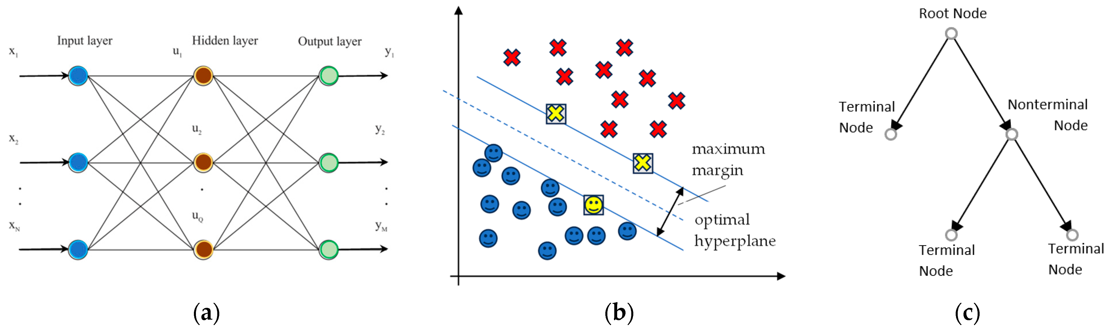
| Machine Learning | Support Vector Machine (SVM) | SVM finds the optimal hyperplane that maximises the margin between classes in high-dimensional space. | Effective for high-dimensional data; Robust to overfitting in many cases. | Requires proper kernel selection; Limited performance with large datasets. | Fault classification using vibration data; Distinguishing between different fault types. | [103,104,105] |
| Machine Learning | Random Forest (RF) | RF uses an ensemble of decision trees trained on various sub-samples of the dataset, and averages to improve prediction accuracy. | Handles large datasets well; Robust to overfitting due to averaging. | Computationally intensive for large trees; Can become biased if some classes dominate. | Classifying complex and non-linear fault patterns; Identifying feature importance for fault diagnosis. | [106,107] |
| Machine Learning | k-Nearest Neighbours (k-NN) | k-NN classifies a data point based on the majority class among its k-nearest neighbours in the feature space. | Simple and intuitive; No training phase required. | Computationally expensive for large datasets; Sensitive to irrelevant features and noisy data. | Fault classification with small and simple datasets; Quick diagnostics in real-time systems. | [108,109] |
| Deep Learning | Convolutional Neural Network (CNN) | CNNs use convolutional layers to automatically extract spatial features from raw data and learn hierarchical representations. | Excellent at feature extraction from raw data; High performance in image and signal processing. | Requires large datasets and computational resources; Less interpretable than traditional methods. | Bearing fault diagnosis using vibration signal images; Automatic feature extraction and classification. | [110,111] |
| Deep Learning | Recurrent Neural Network (RNN) | RNNs handle sequential data and learn temporal dependencies by using feedback loops in the network architecture. | Effective for time-series data; Captures temporal dependencies and dynamics. | Prone to vanishing gradient problems; Requires careful tuning and long training times. | Fault diagnosis from sequential vibration data; Monitoring time-evolving fault characteristics. | [112] |
| Deep Learning | Autoencoder | Autoencoders learn to encode input data into a lower-dimensional representation and then reconstruct the original input. | Useful for unsupervised learning; Can handle unlabelled data for anomaly detection. | Reconstruction quality depends on network complexity; Less effective for supervised classification. | Unsupervised feature learning and anomaly detection; Identifying new or unknown fault types. | [113] |
| Deep Learning | Transfer learning | Transfer knowledge from related tasks to improve fault diagnosis. | Reduces need for large labelled datasets, improves model generalisation. | Requires related source and target domains. | Fault diagnosis with limited labelled data. | [114] |
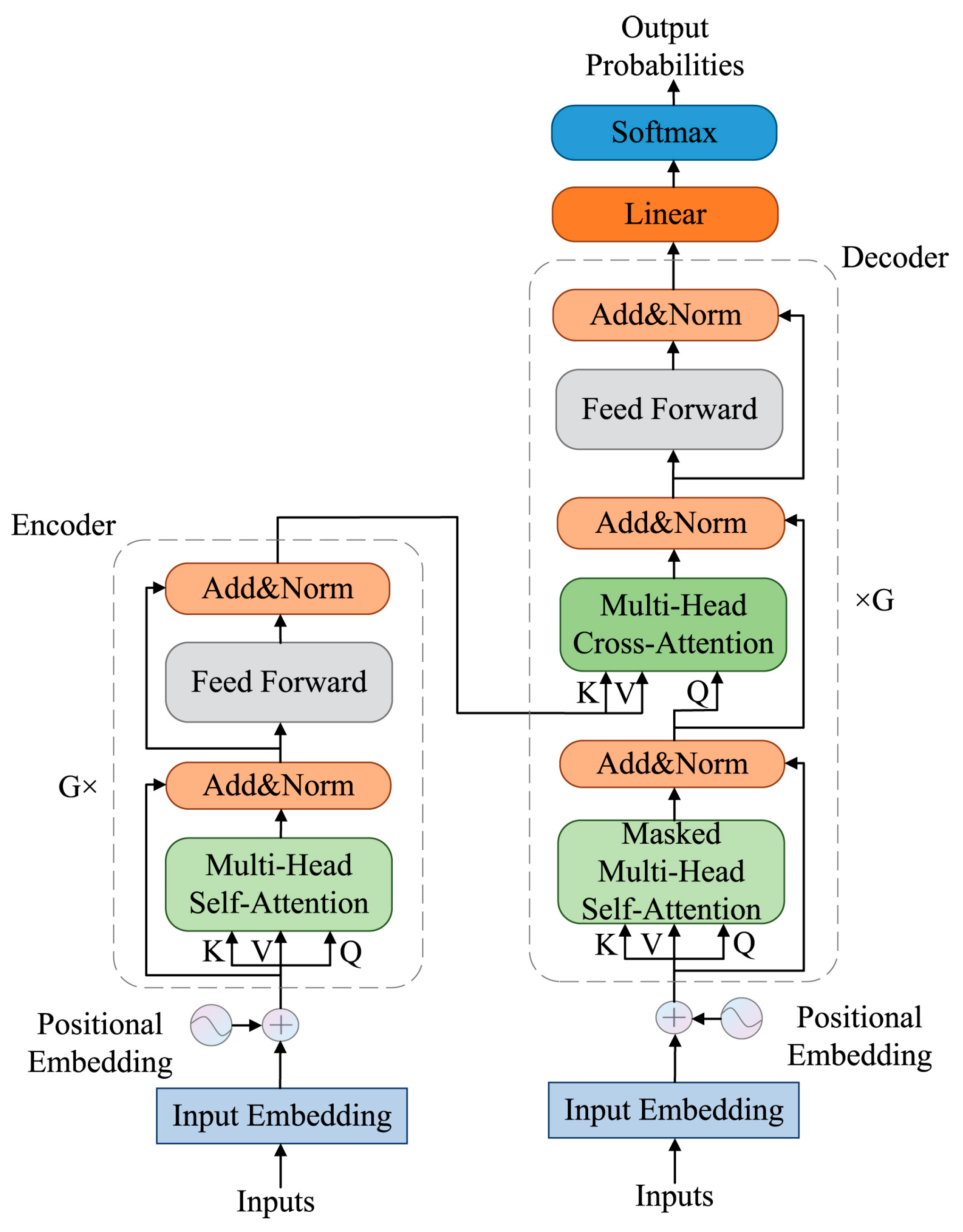
| Deep Learning | Transformer | Leverage self-attention mechanisms to capture complex dependencies. | Handles long-range dependencies, parallelisable training. | Requires large datasets, high computational cost. | Fault diagnosis with complex sequential data. | [115,116] |
| Metaheuristic Optimisation | Genetic Algorithm (GA) | GAs simulate the process of natural selection to optimise feature selection and classification parameters. | Effective for global optimisation; Can handle complex, non-linear problems. | Computationally expensive; Requires careful tuning of parameters. | Optimising feature selection for fault diagnosis. Finding optimal classification parameters. | [62] |
| Metaheuristic Optimisation | Particle Swarm Optimisation (PSO) | PSO mimics the social behaviour of birds or fish to find the optimal solution by sharing information among individuals in a swarm. | Fast convergence to optimal solutions; Simple to implement and understand. | May converge to local optima; Performance sensitive to parameter settings. | Optimising neural network weights for fault classification; Feature selection and parameter tuning. | [117] |
| Metaheuristic Optimisation | Ant Colony Optimisation (ACO) | ACO simulates the foraging behaviour of ants to find optimal paths and solutions by reinforcing successful trails. | Effective for combinatorial optimisation problems; Can explore large solution spaces efficiently. | Slower convergence compared to other methods; Performance dependent on heuristic design. | Optimising fault diagnosis rules and decision-making; Feature selection and optimisation. | [105] |
| Challenges | Methods/Techniques | Publications |
|---|---|---|
| Time-Varying Conditions | Order tracking, angular domain resampling, oscillatory time frequency concentration, time–frequency ridge estimation, adaptive filter, transformer, autoencoder | [79,80,81,82] |
| Measurement Uncertainties | Information fusion, robust statistical methods, noise-tolerant SVM, KNN | [48,111,118,119] |
| Unknown Fault Labels | Unsupervised learning, clustering, semi-supervised learning, autoencoder, transfer learning, domain adaptation, generative adversarial network (GAN), digital twins | [113,120,121] |
| Multiple Bearings (Unknown Locations) | Sensor fusion—data fusion, feature-level fusion, blind source separation | [122] |
| Complex Fault Patterns | Ensemble methods—random forest, hybrid SVM-KNN, CNN-LSTM | [119,120] |
| Year | 2016 | 2017 | 2018 | 2019 | 2020 | 2021 | 2022 | 2023 | 2024 (up to June) |
| Articles | 3 | 15 | 41 | 72 | 157 | 237 | 345 | 398 | 387 |
Disclaimer/Publisher’s Note: The statements, opinions and data contained in all publications are solely those of the individual author(s) and contributor(s) and not of MDPI and/or the editor(s). MDPI and/or the editor(s) disclaim responsibility for any injury to people or property resulting from any ideas, methods, instructions or products referred to in the content. |
© 2024 by the authors. Licensee MDPI, Basel, Switzerland. This article is an open access article distributed under the terms and conditions of the Creative Commons Attribution (CC BY) license (https://creativecommons.org/licenses/by/4.0/).
Share and Cite
Kannan, V.; Zhang, T.; Li, H. A Review of the Intelligent Condition Monitoring of Rolling Element Bearings. Machines 2024, 12, 484. https://doi.org/10.3390/machines12070484
Kannan V, Zhang T, Li H. A Review of the Intelligent Condition Monitoring of Rolling Element Bearings. Machines. 2024; 12(7):484. https://doi.org/10.3390/machines12070484
Chicago/Turabian StyleKannan, Vigneshwar, Tieling Zhang, and Huaizhong Li. 2024. "A Review of the Intelligent Condition Monitoring of Rolling Element Bearings" Machines 12, no. 7: 484. https://doi.org/10.3390/machines12070484
APA StyleKannan, V., Zhang, T., & Li, H. (2024). A Review of the Intelligent Condition Monitoring of Rolling Element Bearings. Machines, 12(7), 484. https://doi.org/10.3390/machines12070484