Abstract
The problem of the insufficient accuracy performance of industrial robots in high-precision manufacturing is addressed in this paper. Firstly, a kinematic error model based on an M-DH model was presented. Secondly, a hybrid observability index O6 was proposed to select the optimal poses for parameter identification. O6 is the combination of O1 and O3. The optimal poses were obtained by using the IOOPS algorithm. Thirdly, the fitness function for parameter identification was established, and the Levenberg–Marquardt (LM) algorithm was applied for the accurate identification of kinematic parameter errors. Finally, several experiments were conducted to evaluate the performance of the proposed hybrid observability index O6. The average position error and average attitude error of Staubli TX60 robot were reduced by 89% and 49%. The results show that the proposed hybrid observability index O6 has great stability and effectiveness for robot calibration.
1. Introduction
Industrial robots have been widely applied in plenty of fields [1,2,3]. The repeat positioning accuracy of industrial robots can reach from 0.01 to 0.1 mm. However, the absolute positioning accuracy is only achieved at a millimeter level. Research shows that the error factors leading to poor accuracy performance of industrial robots include the joint encoder errors, the reducer transmission errors, the kinematic parameter errors, the joint and linkage flexibility errors, and stiffness error caused by robot own weight and external forces, etc. [4,5,6,7,8,9]. The kinematic parameter error is the major error factor that affects the absolute positioning accuracy of industrial robots. Robot calibration technology can improve the accuracy performance of industrial robots [10,11,12].
Robot calibration methods are classified into error-model-based calibration methods and non-model-based calibration methods [13]. The non-model-based calibration methods consider various error factors in an integrative manner. Min K. et al. proposed a stable and highly accurate model-free calibration method by improving the existing kriging error compensation method [14]. However, non-model-based calibration methods cannot compensate errors in real time. Error-model-based calibration methods can be divided into four basic steps: error model establishment, robot error measurement, parameter identification, and error compensation [15]. The error model is established based on several kinematic models, such as the DH model [16], POE model [17], ZRM model [18], etc. Due to the non-singular property and completeness, the M-DH model is the most widely used model in robot calibration technology [19]. There are plenty of measurement devices used for obtaining positioning errors, such as the laser tracker [20,21], the ball bar [22], the stereo vision measurement system [23], and the IMU [24]. The laser tracker is the most commonly used measurement device in robot calibration. In the parameter identification steps, a multivariate optimization objective function is constructed based on the error model. The parameter errors can be identified by the traditional optimization algorithms and intelligent optimization algorithms [25]. Ma L. et al. applied the maximum likelihood method to achieve parameter identification. The proposed method significantly improved the robot’s error [26]. Chen X. et al. proposed an improved multi-objective PSO algorithm for kinematic parameter identification [27]. Except for the properties of the optimization algorithms, the selected measured poses also affect the identification accuracy. Yu Sun et al. studied the factors affecting the accuracy of robot calibration [28]. They proved that an optimal pose selection method can effectively improve the accuracy of robot calibration. In order to evaluate the goodness of the measured poses, five observability indexes—O1, O2, O3, O4, and O5—were proposed [29,30,31,32]. The measured poses are selected based on the criterion of maximizing the observability indexes. The selected measured poses can improve the accuracy performance of robot calibration [33]. The impacts of each observability index on robot calibration were studied in [34,35]. Yu Z. et al. [36] compared the performance of different observability indexes for a 6 DOF serial robot. The results show that O1 has the best performance among the five indexes. Horne A. et al. [37] investigated the performance of different observability indexes by simulating a 2 DOF robotic arm. The results show that O5 and O3 have good and poor performance, respectively. Wang W. et al. [38] proposed a universal observability index to calibrate serial robots. An improved PSO algorithm was used to select the optimal poses. The accuracy performance of surgical robot was effectively improved. However, there are no uniform conclusions about the performance of each observational index. Each observational index has its advantages and disadvantages in different robot configuration. At present, the 6 DOF industrial robots are the most commonly applied in research. Meanwhile, fewer studies have been conducted to investigate the calibration performance of different observation indexes for the 6 DOF industrial robots.
In this paper, a robot calibration method based on the hybrid observability index is proposed. The M-DH kinematic model and the error model are presented in Section 2. Section 3 introduces the different observability indexes and IOOPS algorithm. The IOOPS algorithm is applied to select the optimal measured poses. The performance of different observability indexes has been compared. Based on the analysis results, a hybrid observability index O6 is proposed for robot calibration. Section 4 introduces the LM algorithm to identify the kinematic parameter errors. The experimental results are presented in Section 5. The conclusion of this study and future research are summarized in Section 6.
2. Kinematic Error Model
2.1. M-DH Kinematic Model
As shown in Figure 1A, the industrial robot to be calibrated is the Staubli TX60 robot. The joint coordinate system of the Staubli TX60 robot is illustrated in Figure 1B. The M-DH kinematic model is used to describe the mathematical model of the robot. Based on the definition of the M-DH kinematic model, the transformation matrix Ai between the adjacent joints is given as Equation (1).
where ai, di, αi, θi, and βi (i = 1, 2, …, 6) are the nominal values of the link length, the link offset, the link twist angle, the joint angle, and the joint torsion angle of the i-th joint, respectively. s and c are the abbreviations of sin() and cos(), respectively.
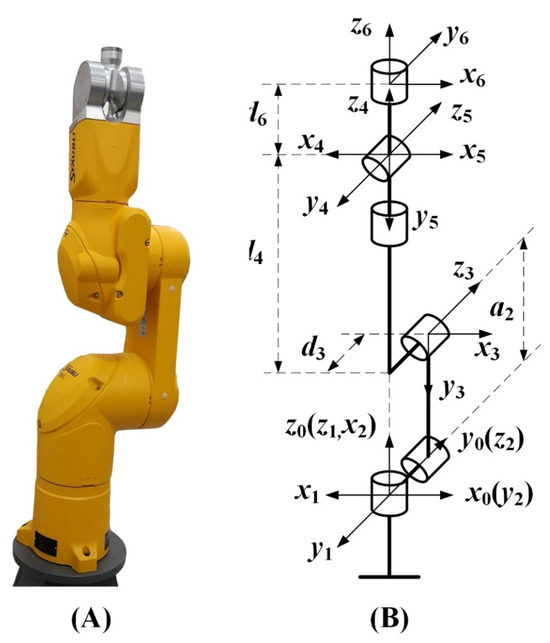
Figure 1.
StaubliTX60 industrial robot (A) and the definition of the joint coordinate system (B).
Therefore, the nominal pose matrix Tn of the industrial robot can be obtained by Equation (2).
where Rn and Pn are the nominal rotation matrix and the nominal displacement vector, respectively. n denotes the nominal kinematic parameters.
The nominal M-DH parameters of the Staubli TX60 robot are shown in Table 1. However, due to errors introduced by manufacturing and assembly, the kinematic parameters of the industrial robot are inconsistent with the nominal values. The errors of the kinematic parameters ai, di, αi, θi, and βi are defined as Δai, Δdi, Δαi, Δθi, and Δβi. The actual pose matrix Tr of the industrial robot can be obtained by Equation (3).
where Rr and Pr are the actual rotation matrix and the actual displacement vector, respectively. r denotes the actual kinematic parameters.

Table 1.
Nominal values of the M-DH kinematic model of the Staubli TX60 robot.
2.2. Pose Error Model
The pose error of the industrial robot is defined as ∆T, which is the difference between the actual pose Tr and the nominal pose Tn.
With respect to the kinematic parameters, the partial differentiation is performed on each column vector of the pose matrix T. The high-order differential terms are ignored. Therefore, the linearized kinematic error model is given as (5).
where H is the Jacobi matrix of kinematic parameters, . N is the number of measured poses. , is the error vector of the kinematic parameters to be identified.
3. Pose Selection Based on a Hybrid Observability Index
3.1. Overview of Observability Indexes
The measured poses used for parameter identification largely influence the calibration results. In order to optimize the effect of robot calibration, five observational indexes were proposed to evaluate the quality of the measured poses. The observational indexes are calculated based on the none-zero singular values of the Jacobi matrix H. The singular value decomposition (SVD) of the Jacobi matrix H is defined as
where U and V are all orthogonal matrices. . ∑ is a diagonal matrix composed of singular values. .
where the value σi (i = 1, 2, …, 24) is the none-zero singular value of the Jacobi matrix H. σ1 ≥ σ2 ≥ σ3 ≥ … ≥ σ24.
By substituting the above Equation (7) into (5), the expression is given as follows:
From Equations (7) and (8), the singular values σi of the Jacobi matrix H correspond to the axes of the hyperellipsoid. It represents the sensitivity of each kinematical parameter to the pose. Menq C. [29] proposed the observability index O1, defined as (9). O1 is associated with hyperellipsoid volume. The larger O1 is, the larger the hyperellipsoid volume is.
where n is the number of calibration poses. L is the number of kinematic parameters to be identified.
Driels M. [30] proposed the observability index O2, defined as (10). O2 represents roundness of the hyperellipsoid.
Nahvi A. [31] proposed an observability index O3. O3 is the smallest singular value. Nahvi A also proposed a hybrid observability index O4.
Sun Y. [32] proposed the observability index O5. Maximizing the value of O5 ensures that the hyperellipsoid volume is maximized.
3.2. Selecting Optimal Poses for Identification
The iterative one-by-one pose search (IOOPS) algorithm is derived from the DETMAX algorithm [39]. The IOOPS algorithm can search for a given number of optimal poses within an infinite pose set. The flowchart of the IOOPS algorithm is shown in Figure 2. Firstly, an initial pose set U is randomly determined. The pose set U is divided into the selected pose set γm and alternative pose set γR. Secondly, the add algorithm and remove algorithm are used to select the optimal poses. The parameter descriptions of the IOOPS algorithm are shown in Table 2. Details of the add algorithm and remove algorithm are shown as follows:
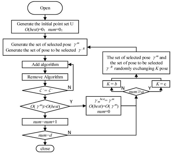
Figure 2.
Flowchart of the IOOPS algorithm.
Table 2.
Parameter description of the IOOPS algorithm.
In the add algorithm, the pose ζi(i = 1, 2,…, n) is taken sequentially from the alternative pose set γR. If the max{O6(γm + ζi)} is maximum, the ζi is denoted as ζ+. The selected pose set γm adds one pose, becoming γm+1. Thus, γm+1 = γm + ζ+.
In the remove algorithm, the pose ζi(i = 1, 2,…, n) is removed sequentially from the selected pose γm+1. If the max{O6(γm+1 − ζi)} is maximum, the ζi is denoted as ζ−. The selected pose set γm+1 deletes one pose. The selected pose becomes γm. γm = γm+1 − ζ−.
3.3. A Novel Hybrid Observability Index
In order to analyze the performance of different observability indexes, the four independent observability indexes (O1, O2, O3, and O5) are chosen for comparison. As given in Equation (12), the observability index O4 is a combination of O2 and O3. Therefore, the observability index O4 is not discussed. In the analysis process, 50 optimal poses are first selected from 200 measured poses with the IOOPS algorithm based on the four different observability indexes. The remaining 150 measured poses are used for validating the identified kinematic models. Secondly, the kinematic parameter errors are identified by the LM algorithm. The attitude errors and the positioning errors before and after robot calibration are shown in Figure 3 and Figure 4. In this paper, the average comprehensive position error (EACPE) and the average comprehensive attitude error (EACAE) are defined to evaluate the accuracy performance of the industrial robot.
where M denotes the number of measured poses,,, and are the position errors in the x-axis, y-axis, and z-axis. , , and are the attitude errors in the x-axis, y-axis, and z-axis.
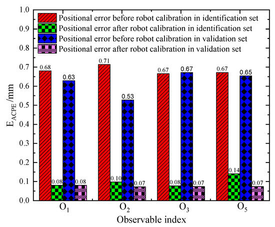
Figure 3.
EACPE before and after robot calibration based on different observability indexes.
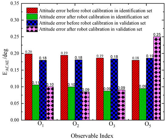
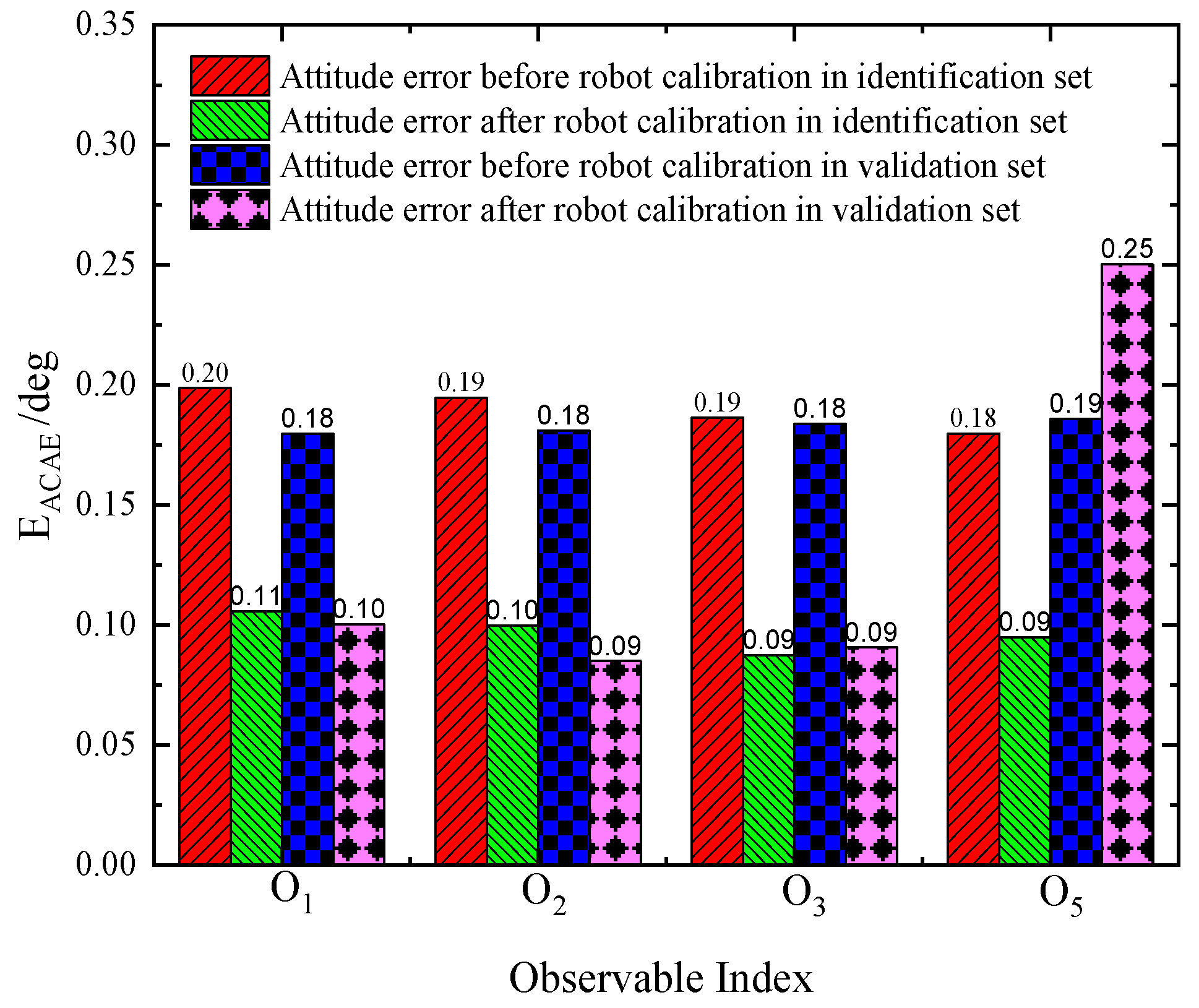
Figure 4.
EACAE before and after robot calibration based on different observability indexes.
Table 3 presents the improvement ratio of the attitude accuracy and positioning accuracy in the identification and validation sets. As shown in Table 3, O5 is worst in terms of EACAE in validation set. O1 and O3 are better in terms of EACPE in both identification and validation sets. Moreover, O3 is better in terms of EACAE in both identification and validation sets. Experimental results show that O1 and O3 have better performance. The poses selection is an optimized procedure which maximizes the observability index value. To ensure the maximum values of O1 and O3 simultaneously, a hybrid observability index O6 is proposed. The expression of O6 is given as (16).
where k is the coefficient. The coefficient is determined, as described in Section 5.1.
Table 3.
Iimprovement ratio of Robot positioning and attitude accuracy for different observability index.
4. Parameters Identification
There are plenty of algorithms for kinematic parameter identification, of which the most commonly employed is the least squares (LS) optimization algorithm. The formula of the LS optimization algorithm is given based on Equation (17) as follows:
When the matrix HTH is invertible or a pathological matrix, the LS optimization algorithm cannot find the correct solution. The Levenberg–Marquardt (LM) optimization algorithm is an improvement on the LS optimization algorithm. The LM optimization algorithm can avoid this problem through adding a unit matrix. In this paper, the LM algorithm is used to identify the kinematic parameter errors. The formula of the LM optimization algorithm is given as follows:
where μ is a coefficient with an initial value of 0.01. I is the unit matrix.
Based on the M-DH kinematic error model obtained above, d2, β1, β3, β4, β5, and β6 are no need to be identified. Therefore, only 24 kinematic parameter errors need to be identified. As is well known, the position error and attitude error have a great difference in dimension and magnitude. To simplify the optimization process, the position error fitness function and the attitude error fitness function are fused in (19).
where N is the number of measured poses, N = 50. L is the adjustment factor, which is used to balance position error and attitude vector in the objective function, L = 100.
5. Experiment Results
5.1. Robot Calibration Experimental Platform
As shown in Figure 5, the industrial robot calibration system is established in this paper. The laser tracker Leica AT960 is used to measure the poses of the Staubli TX60 robot. The T-Mac tool of the laser tracker is installed on the industrial robot flange. Spatial Analyzer and Matlab are used for processing the measured data. The positioning measurement uncertainty of the laser tracker is 15 μm + 6 μm/m × Dm. D indicates the distance between the laser tracker and the T-Mac tool. The measured distance in the experiment is nearly 1.5 m. The Staubli TX60 robot to be calibrated in this paper has a repetitive positioning accuracy of ±0.02 mm and a rated load of 3 Kg. The transformation relation between the measurement coordinate frame and the base coordinate frame can be obtained through the method presented in [40]. The experimental measurement procedure is as follows:
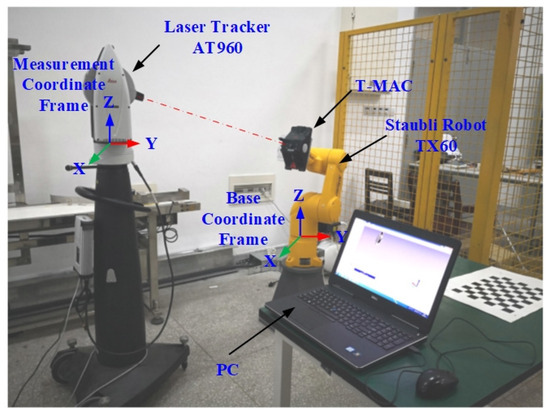
Figure 5.
The industrial robot calibration system.
- (1)
- The transformation between the base coordinate frame of the Staubli TX60 robot and the measurement coordinate frame of the laser tracker Leica AT960.
- (2)
- The transformation between the frame of T-Mac tool and the tool frame of the Staubli TX60 robot.
- (3)
- The base coordinate frame of the Staubli TX60 robot was used as the reference coordinate system.
The measurement processes involved in this paper are in accordance with the ISO-9283 performance specification for industrial robots and its test method standard [41]. There are 1200 measured poses selected randomly in the front motion space of the robot. The motion space is a cube of which length is 1 m. The measured poses are selected by the RoboDyn software. The measured poses are distributed in the measured motion space as much as possible.
5.2. Robot Calibration Based on the Proposed Hybrid Observability Index
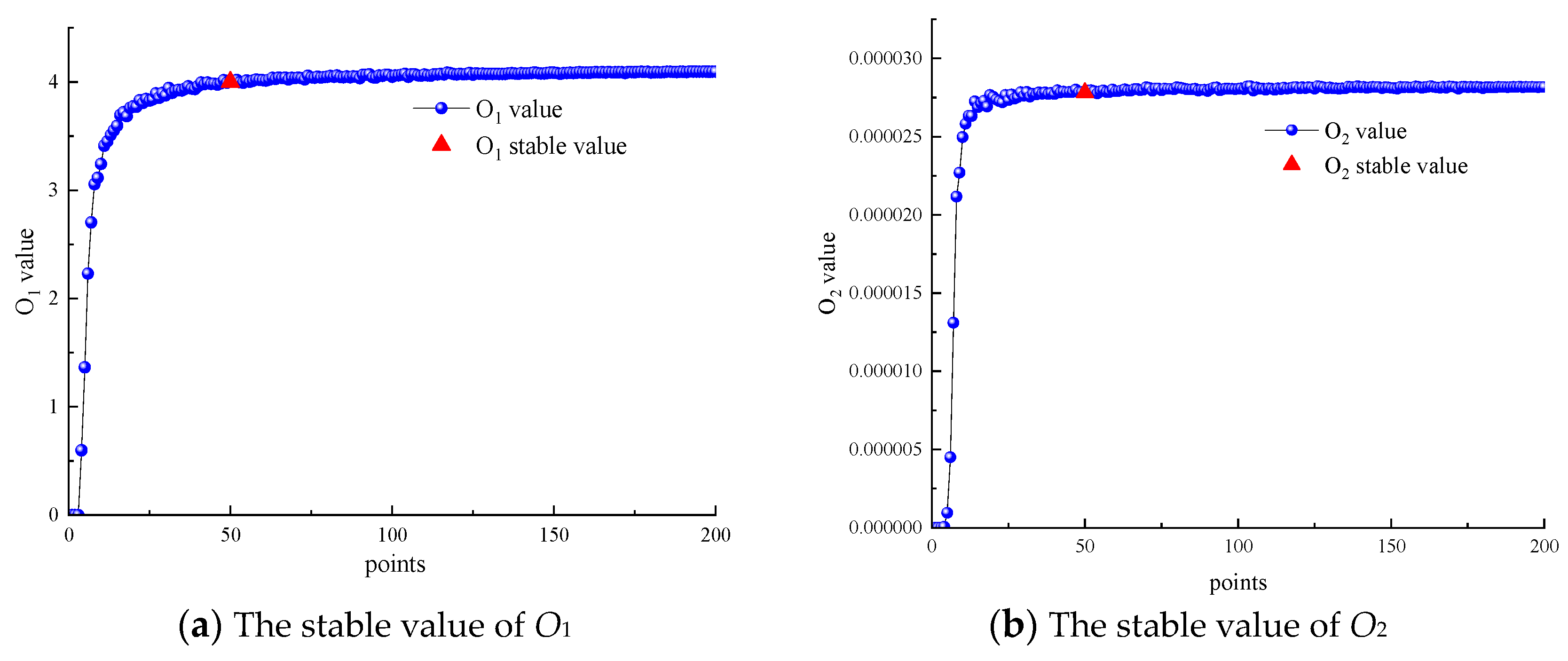
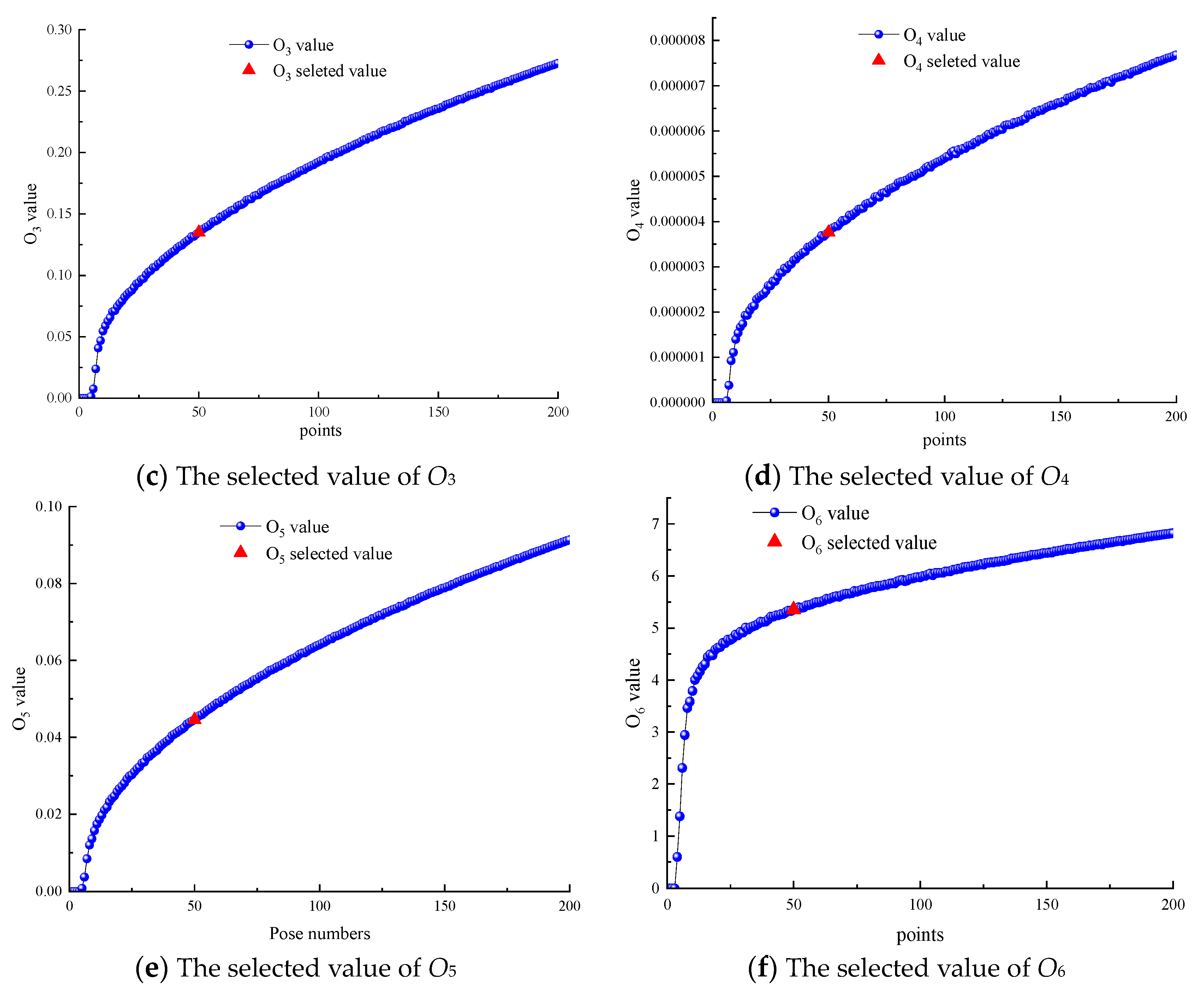
When the number of poses increases to a certain number, the identification accuracy does not increase. Therefore, the optimal number of poses should firstly be determined by the selection algorithm. In the algorithm, two random poses are selected among 200 measured poses initially. The six observability indexes of the selected poses are calculated. The above process is repeated T times. The number of randomly selected poses gradually increases. As shown in Figure 6a,b, it can be seen that the observability indexes O1 and O2 steadily increase when the number of poses reaches 50. From Figure 6c,f, it is shown that the observability indexes O3 to O6 increase monotonically. Therefore, the optimal number of poses is set as 50 for cross-comparison and fast calibration.
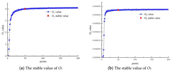
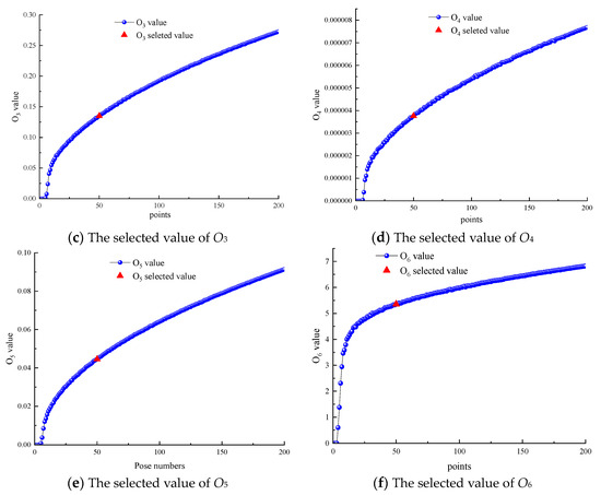
Figure 6.
Determination of stabilization values for individual observational indices.
As shown in Figure 6a,c, the ratio of O1 and O3 stable values is closed to 10. Therefore, the coefficient k in Equation (16) is initially set as 10. To compare the performance and the stability of the proposed hybrid observability index O6, 1200 measured poses are divided into six groups. Five groups are selected to verify the stability of the proposed hybrid observability index O6, and the other one group is used to verify its performance.
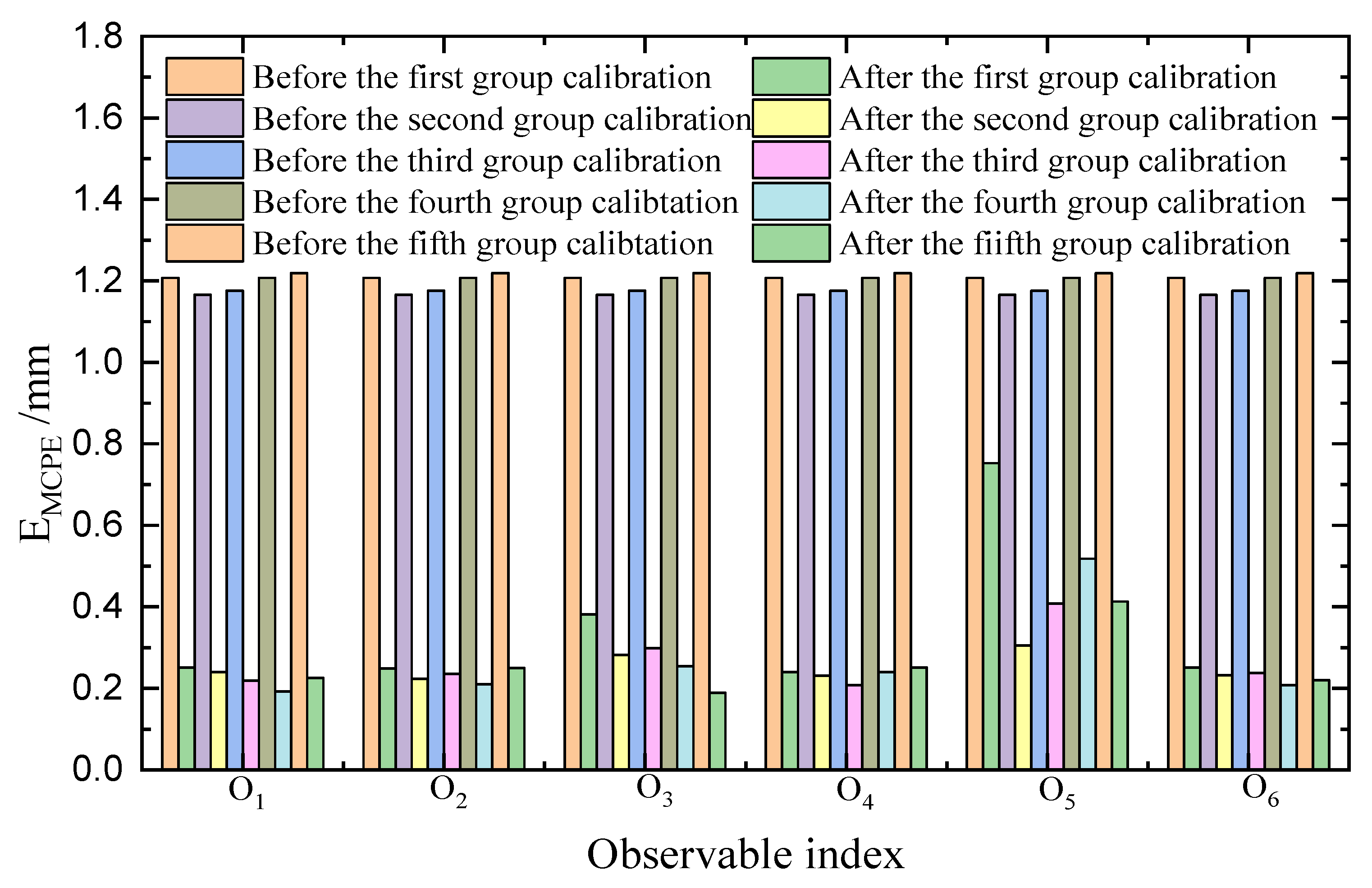
Firstly, the IOOPS algorithm is applied to select 50 optimal poses from 200 measured poses in each group based on the proposed O6 index. The optimal poses are used for parameter identification, and the remaining 150 poses are used for verification. Secondly, the parameter identification is conducted through the LM algorithm. The EACPE of the industrial robot after calibration was used to evaluate the comprehensive error of the method. Moreover, the maximum comprehensive position error (EMCPE) and the maximum comprehensive attitude error (EMCAE) are defined to evaluate the accuracy performance of the industrial robot.
where Max denotes the maximum value in the results.
The results of robot calibration are shown in Figure 7 and Figure 8. EACPE of the O1, O3, and O6 are almost identical. The EMCPE of the proposed O6 is better than O3. As summarized in Table 4, it can be seen that the calibration performance of the proposed hybrid observability index O6 is more stable than other observability indexes.
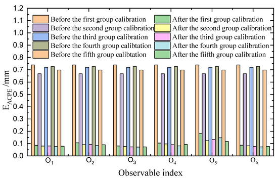
Figure 7.
Average comprehensive positioning error of the robot with different observability indexes.
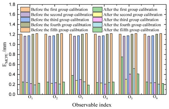
Figure 8.
Maximum comprehensive positioning error of the robot with different observability indexes.
Table 4.
Robot positioning and attitude enhancement accuracy for different observability indexes.
To verify the accuracy performance of the proposed hybrid observability index O6, 50 optimal poses were firstly selected from the sixth group. The identification results of the kinematic parameter errors of the Staubli TX60 robot are given in Table 5. The EACPE and EACAE of the Staubli TX60 robot is reduced from (0.716 mm, 0.167°) to (0.082 mm, 0.077°). The position and attitude accuracy performances of the Staubli TX60 robot are improved by 89% and 49%. The EMCPE and EMCAE of the Staubli TX60 robot is reduced from (1.187 mm, 0.281°) to (0.22 mm, 0.177°) by the LM algorithm. The position and attitude accuracy performances of the Staubli TX60 robot are improved by 81% and 37%. It can be seen that highly accurate parameter identification can be achieved based on the proposed hybrid observability index O6.
Table 5.
The identified parameter errors of the calibrated robot.
5.3. Comparison of Robot Calibration Algorithms
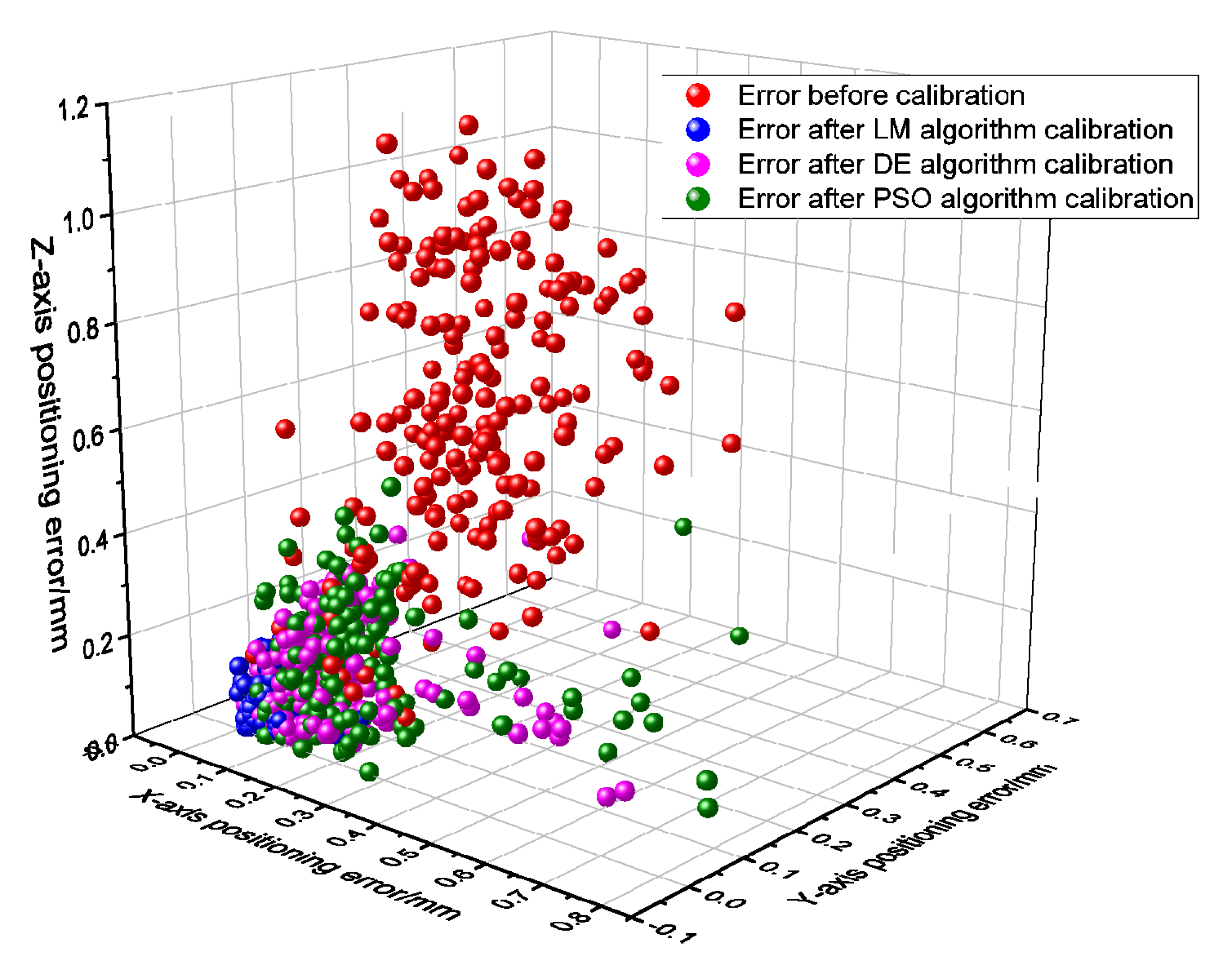
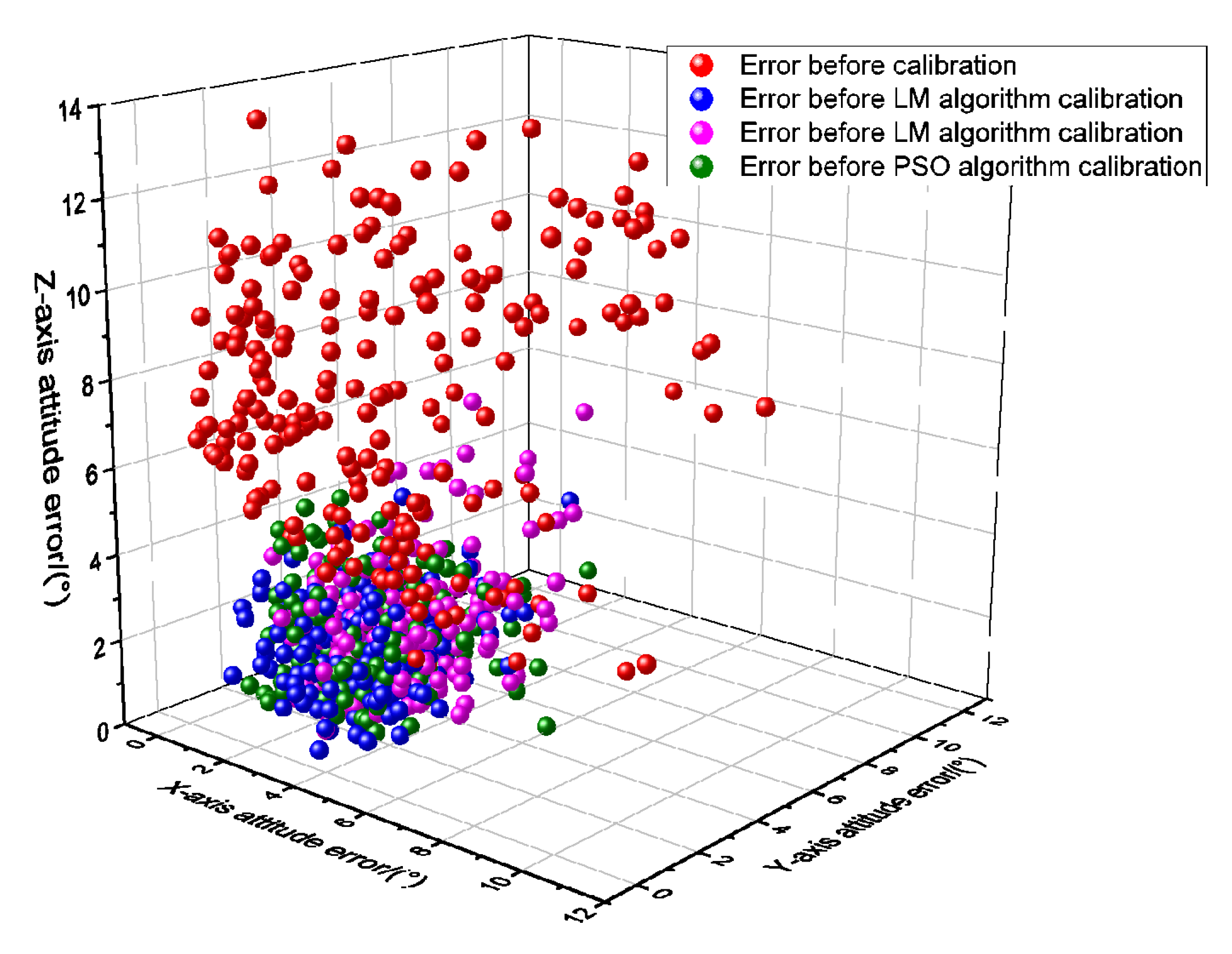
The calibration performance of the LM, PSO, and DE algorithms are compared. The results are illustrated in Figure 9 and Figure 10. The EACPE and EACAE of the Staubli TX60 robot are reduced from (0.716 mm, 0.167°) to (0.2396 mm, 0.080°) by the PSO algorithm. Meanwhile, the EACPE and EACAE of the Staubli TX60 robot are reduced from (0.716 mm, 0.167°) to (0.1935 mm, 0.097°) by the DE algorithm. In summary, the accuracy of the parameters identified using the LM algorithm is better than the PSO and DE algorithms.

Figure 9.
Industrial robot positioning error before and after calibration.

Figure 10.
Industrial robot attitude error before and after calibration.
6. Discussion
The observability index is actually a loss function for optimizing the selected poses used for identification. Five observability indexes were investigated for the calibration of various robots. The calibration effectiveness of the typical observability indexes for six DOF serial industrial robots is compared through the experiments. Studies also show that O1 has have better performance. The experimental results in this paper show that the selected poses based on O1 and O3 are relatively effective in positioning accuracy; meanwhile, O3 is more effective in attitude accuracy. Therefore, both O1 and O3 were used as criteria for selecting measured poses, and the positioning and attitude accuracy of the calibration performance both improved. Based on the handling of objective functions in multi-objective optimization methods, a hybrid observability index O6 is expressed as (16). Firstly, the target number of the selected poses is determined. The 50 selected poses can ensure the calibration efficiency and cross-comparison. Secondly, the coefficient k in Equation (16) is determined as 10. The performance of each observability index is compared with six different groups of measured poses. As shown in Figure 7 and Figure 8, the positioning accuracy EACPE and EMCPE of O6 is consistent with O1. Moreover, the attitude accuracy EACAE and EMCAE of O6 is also consistent with O1. As is well known, the coefficient k in Equation (16) can balance the effects of the observability indexes O1 and O3. The coefficient k can be adjusted to obtain a better performance in both positioning accuracy and attitude accuracy. However, it is hard to find the best solution of the coefficient k.
The selected measured poses are applied to identify the kinematic parameters with different optimization algorithms. The comparison results show that the LM algorithm is better than the PSO and DE algorithms.
7. Conclusions
This paper proposes a hybrid observability index for selecting the optimal poses to improve the accuracy performance of the industrial robot. Firstly, the kinematic error model of the robot is constructed based on the M-DH model. Secondly, the performance of each observability index is evaluated, and the proposed hybrid observability index O6 is defined. O6 is the linear combination of O1 and O3. The optimal poses is obtained by using the IOOPS algorithm. Thirdly, the fitness function and identification algorithm are presented based on the kinematic error model. Finally, several experiments have been conducted to evaluate the performance of the proposed hybrid observability index O6. Based on the proposed hybrid observability index O6, the ACPE and ACAE of the Staubli TX60 robot is reduced from (0.716 mm, 0.167°) to (0.082 mm, 0.077°). The average position error and average attitude error of the Staubli TX60 robot were reduced by 89% and 49%. The results show that the proposed hybrid observability index O6 has great stability and effectiveness for robot calibration.
Future research will focus on the multi-objective optimization algorithm for selecting measured poses based on the two observability indexes O1 and O3. Moreover, the stiffness error compensation of the self-weight and external loads can make the robot suitable for complex working conditions. It will also be the primary focus of research in the future.
Author Contributions
Conceptualization, T.X.; methodology, H.Z.; software, B.D., C.G. and G.Q.; validation, B.D., C.G. and G.Q.; formal analysis, B.D., C.G. and G.Q.; investigation, T.X.; resources, G.Q.; data curation, G.Q.; writing—original draft preparation, T.X.; writing—review and editing, H.Z.; visualization, C.G.; supervision, H.Z.; project administration, G.Q.; funding acquisition, T.X. and G.Q. All authors have read and agreed to the published version of the manuscript.
Funding
This research reported in this paper was carried out at College of Civil Aviation, Nanjing University of Aeronautics and Astronautics, and School of Automation, Nanjing Institute of Technology. This work was supported in part by Natural Science Foundation of China under Grant 51905258, China Postdoctoral Science Foundation 2019M650095.
Data Availability Statement
The data presented in this study are available on request from the corresponding author. The data are not publicly available due to our project has not finished yet.
Conflicts of Interest
The authors declare that there are no conflicts of interest regarding the publication of this article.
References
- Wang, Z.; Cao, B.; Xie, Z.; Ma, B.; Sun, K.; Liu, Y. Kinematic Calibration of a Space Manipulator Based on Visual Measurement System with Extended Kalman Filter. Machines 2023, 11, 409. [Google Scholar] [CrossRef]
- Yuan, Y.; Sun, W. An integrated kinematic calibration and dynamic identification method with only static measurements for serial robot. IEEE/ASME Trans. Mechatronics 2023, 28, 2762–2773. [Google Scholar] [CrossRef]
- Borboni, A.; Pagani, R.; Sandrini, S.; Carbone, G.; Pellegrini, N. Role of reference frames for a safe human–robot interaction. Sensors 2023, 23, 5762. [Google Scholar] [CrossRef] [PubMed]
- Wang, X.; Xie, L.; Jiang, M.; He, K.; Chen, Y. Kinematic calibration and feedforward control of a heavy-load manipulator using parameters optimization by an ant colony algorithm. Robotica 2024, 42, 728–756. [Google Scholar] [CrossRef]
- Gharaaty, S.; Shu, T.; Joubair, A.; Xie, W.F.; Bonev, I.A. Online pose correction of an industrial robot using an optical coordinate measure machine system. Int. J. Adv. Robot. Syst. 2018, 15. [Google Scholar] [CrossRef]
- Chen, T.; Li, S.; Luo, X. A Highly-Accurate Robot Calibration Method with Line Constraint. In Proceedings of the IEEE International Conference on Networking, Sensing and Control, Marseille, France, 25–27 October 2023. [Google Scholar]
- Gao, G.; Sun, G.; Na, J.; Guo, Y.; Wu, X. Structural parameter identification for 6 DOF industrial robots. Mech. Syst. Signal Process. 2018, 113, 145–155. [Google Scholar] [CrossRef]
- Chen, B.; Wang, Y.; Hu, S.; Tao, Z.; Qi, J. A whole-path posture optimization method of robotic grinding based on multi-performance evaluation indices. Robot. Comput. Manuf. 2024, 89, 102787. [Google Scholar] [CrossRef]
- Carbone, G.; Ceccarelli, M. Comparison of indices for stiffness performance evaluation. Front. Mech. Eng. China 2010, 5, 270–278. [Google Scholar] [CrossRef]
- Asif, S.; Webb, P. Managing Delays for Realtime Error Correction and Compensation of an Industrial Robot in an Open Network. Machines 2023, 11, 863. [Google Scholar] [CrossRef]
- Veitschegger, W.K.; Wu, C. Robot calibration and compensation. IEEE J. Robot. Autom. 1988, 4, 643–656. [Google Scholar] [CrossRef]
- Roth, Z.; Mooring, B.; Ravani, B. An overview of robot calibration. IEEE J. Robot. Autom. 1987, 3, 377–385. [Google Scholar] [CrossRef]
- Nubiola, A.; Bonev, I.A. Absolute robot calibration with a single telescoping ballbar. Precis. Eng. 2014, 38, 472–480. [Google Scholar] [CrossRef]
- Min, K.; Ni, F.; Chen, Z.; Liu, H.; Lee, C.-H. A robot positional error compensation method based on improved kriging interpolation and kronecker products. IEEE Trans. Ind. Electron. 2023, 71, 3884–3893. [Google Scholar] [CrossRef]
- Hultman, E.; Leijon, M. Six-Degrees-of-Freedom (6-DOF) Work Object Positional Calibration Using a Robot-Held Proximity Sensor. Machines 2013, 1, 63–80. [Google Scholar] [CrossRef]
- Denavit, J.; Hartenberg, R.S. A kinematic notation for lower-pair mechanisms based on matrices. J. Appl. Mech. 1955, 22, 215–221. [Google Scholar] [CrossRef]
- Liu, H.; Zhu, W.; Dong, H.; Ke, Y. An improved kinematic model for serial robot calibration based on local POE formula using position measurement. Ind. Robot. Int. J. 2018, 45, 573–584. [Google Scholar] [CrossRef]
- Gupta, K.C. Solution Manual for Mechanics and Control of Robots; Springer: Berlin, Germany, 2012. [Google Scholar]
- Hayati, S.A. Robot arm geometric link parameter estimation. In Proceedings of the 22nd IEEE Conference on Decision and Control, San Antonio, TX, USA, 14–16 December 1983. [Google Scholar]
- Qiao, G.; Jiang, X.; Nie, X.; Gao, C. Accuracy Improvement for Industrial Robot Based on Joint Position Sensitive Virtual Tool Transformation Fitting Method. In Proceedings of the 6th International Conference on Robotics, Control and Automation Engineering, Suzhou, China, 3–5 November 2023. [Google Scholar]
- Zhao, D.; Dong, C.; Guo, H.; Tian, W. Kinematic calibration based on the multicollinearity diagnosis of a 6-DOF polishing hybrid robot using a laser tracker. Math. Probl. Eng. 2018, 2018, 5602397. [Google Scholar] [CrossRef]
- Slamani, M.; Joubair, A.; Bonev, I.A. A comparative evaluation of three industrial robots using three reference measuring techniques. Ind. Robot. Int. J. 2015, 42, 572–585. [Google Scholar] [CrossRef]
- Shen, C.; Chen, Y.; Chen, B.; Qiao, Y. A novel robot kinematic calibration method based on common perpendicular line model. Ind. Robot. Int. J. 2018, 45, 766–775. [Google Scholar] [CrossRef]
- Du, G.; Zhang, P. IMU-based online kinematic calibration of robot manipulator. Sci. World J. 2013, 2013, 139738. [Google Scholar] [CrossRef]
- Lin, Y.; Zhao, H.; Ding, H. Posture optimization methodology of 6R industrial robots for machining using performance evaluation indexes. Robot. Comput. Integr. Manuf. 2017, 48, 59–72. [Google Scholar] [CrossRef]
- Ma, L.; Bazzoli, P.; Sammons, P.M.; Landers, R.G.; Bristow, D.A. Modeling and calibration of high-order joint-dependent kinematic errors for industrial robots. Robot. Comput. Manuf. 2018, 50, 153–167. [Google Scholar] [CrossRef]
- Chen, X.; Zhan, Q. The kinematic calibration of a drilling robot with optimal measurement configurations based on an improved multi-objective PSO algorithm. Int. J. Precis. Eng. Manuf. 2021, 22, 1537–1549. [Google Scholar] [CrossRef]
- Sun, Y.; Hollerbach, J.M. Active robot calibration algorithm. In Proceedings of the IEEE International Conference on Robotics and Automation, Pasadena, CA, USA, 19–23 May 2008. [Google Scholar]
- Menq, C.-H.; Borm, J.-H.; Lai, J.Z. Identification and observability measure of a basis set of error parameters in robot calibration. J. Mech. Des. 1989, 111, 513–518. [Google Scholar] [CrossRef]
- Driels, M.R.; Pathre, U.S. Significance of observation strategy on the design of robot calibration experiments. J. Robot. Syst. 1990, 7, 197–223. [Google Scholar] [CrossRef]
- Nahvi, A.; Hollerbach, J.M. The noise amplification index for optimal pose selection in robot calibration. In Proceedings of the IEEE International Conference on Robotics and Automation, Minneapolis, MN, USA, 22–28 April 1996. [Google Scholar]
- Sun, Y.; Hollerbach, J.M. Observability index selection for robot calibration. In Proceedings of the IEEE International Conference on Robotics and Automation, Pasadena, CA, USA, 19–23 May 2008. [Google Scholar]
- Slamani, M.; Makri, H.; Boudilmi, A.; Bonev, I.A.; Chatelain, J.-F. Calibration strategies for enhancing accuracy in serial industrial robots for orbital milling applications. Ind. Robot. Int. J. 2024, 51, 558–569. [Google Scholar] [CrossRef]
- Jiang, Z.; Huang, M.; Tang, X.; Song, B.; Guo, Y. Observability index optimization of robot calibration based on multiple identification spaces. Auton. Robot. 2020, 44, 1029–1046. [Google Scholar] [CrossRef]
- Jia, Q.; Wang, S.; Chen, G.; Wang, L.; Sun, H. A novel optimal design of measurement configurations in robot calibration. Math. Probl. Eng. 2018, 2018, 4689710. [Google Scholar] [CrossRef]
- Yu, Z.; Wu, X.; Wang, F. Kinematic Calibration Method for Six-Hard point Positioning Mechanisms Using Optimal Measurement Pose. Appl. Sci. 2023, 13, 4824. [Google Scholar] [CrossRef]
- Horne, A.; Notash, L. Comparison of pose selection criteria for kinematic calibration through simulation. In Proceedings of the 5th International Workshop on Computational Kinematics, Duisburg, Germany, 6 October 2009. [Google Scholar]
- Wang, W.; Song, H.; Yan, Z.; Sun, L.; Du, Z. A universal index and an improved PSO algorithm for optimal pose selection in kinematic calibration of a novel surgical robot. Robot. Comput. Manuf. 2018, 50, 90–101. [Google Scholar] [CrossRef]
- Daney, D.; Papegay, Y.; Madeline, B. Choosing measurement poses for robot calibration with the local convergence method and tabu search. Int. J. Robot. Res. 2005, 24, 501–518. [Google Scholar] [CrossRef]
- Qiao, G.; Sun, D.; Song, G.; Wen, X.; Wei, Z.; Song, A. A rapid coordinate transformation method for serial robot calibration system. J. Mech. Eng. 2020, 56, 1–8. [Google Scholar]
- ISO 9283; Manipulating Industrial Robots–Performance Criteria and Related Test Methods. International Organization for Standardization: Geneva, Switzerland, 1998.


Disclaimer/Publisher’s Note: The statements, opinions and data contained in all publications are solely those of the individual author(s) and contributor(s) and not of MDPI and/or the editor(s). MDPI and/or the editor(s) disclaim responsibility for any injury to people or property resulting from any ideas, methods, instructions or products referred to in the content. |
© 2024 by the authors. Licensee MDPI, Basel, Switzerland. This article is an open access article distributed under the terms and conditions of the Creative Commons Attribution (CC BY) license (https://creativecommons.org/licenses/by/4.0/).