A Method to Obtain Frequency Response Functions of Operating Mechanical Systems Based on Experimental Modal Analysis and Operational Modal Analysis

Abstract

The characteristics of a mechanical structure under operating conditions may differ from those in a static state. It is often more desirable to obtain the frequency response function (FRF) of the operating structure in engineering applications. While operational modal analysis (OMA) can estimate modal parameters during operation, it fails to provide mass-normalized mode shapes for FRF synthesis. This paper presents a new method using experimental modal analysis (EMA) to compensate for the absent information in OMA. It categorizes operational mode shapes into changed ones and those that remain the same compared to the static state, applying different scaling techniques accordingly. This method adapts to changes in dynamic characteristics without altering the operating conditions. Stability is emphasized throughout the process. Two examples are provided to verify the method, considering noise and incompleteness in measurement, and disturbances in dynamic properties. The proposed method is proven to be feasible and reliable to capture the changes in operational FRFs.

1. Introduction

Frequency response function (FRF) is a powerful tool for structural dynamics engineers, used in various applications such as physical parameter identification [1], finite element method (FEM) model updating [2], structure health monitoring [3], load estimation [4,5] and structure response simulation [6,7]. Typically, the system is assumed to be linear time-invariant, and hence FRFs are measured in a non-operating state. By measuring input forces from artificial excitation equipment, such as impact hammers or shakers, and capturing the output responses of target degrees of freedom (DOFs), FRFs can be easily acquired through the H₁, H₂ or H_v estimator. To facilitate testing and eliminate operational excitation that is too complex to model or measure [8], FRF estimation is, in turn, often required to be performed in a static state. These kinds of FRFs will be referred to as conventional FRFs (CFRFs) in the followings.

In reality, however, FRFs may vary significantly with changes in the dynamic properties depending on the exact operating state. A good example is wind turbines [9], whose modal frequencies are heavily influenced by the rotation speed, due to centripetal and Coriolis forces, which result in tension stiffening. Another extensively studied field is metal processing. The dynamics of a machine tool structure is found to be a function of the tool position and spindle speed [10,11,12], causing the FRFs during actual machining operations to differ substantially from those in a static state. Similar phenomena have been observed in industrial robots [13,14]. In the automobile industry, the variation in FRFs is considerable and complicated in noise and vibration problems. This can be partially attributed to the transmission characteristics of rubber interconnection components, whose dynamic stiffness is amplitude-dependent [15]. Tires add further complexity due to additional operational factors such as rolling speed, static pre-load, inflation pressure and temperature [16,17,18]. Furthermore, the changes in boundary conditions are also non-negligible and may bring in errors if CFRFs are used in vibration and noise analysis for a running car [19]. In summary, numerous mechanical devices exhibit different dynamic characteristics under real-life operating conditions because of factors such as varying spin speeds, loads, vibration amplitudes and temperatures. Consequently, their FRFs change compared to their static states, highlighting the pressing need for Operational FRFs (OFRFs) to replace CFRFs.

Up until now, most studies estimate operational FRF using operational modal analysis (OMA) [20,21]. Unlike traditional experimental modal analysis (EMA) based on CFRFs, OMA needs only vibration response data to extract modal parameters under real operating conditions [22,23]. But, just due to the absence of input information, operational modes cannot be mass-normalized, and thus cannot be further used to synthesize FRFs [24]. To address this issue, several approaches based on structural dynamic modification (SDM), primarily various mass-change strategies, have been proposed [25,26,27], provided the structure is linear. Most of them assume that a perturbation in the mass matrix does not affect the mode shapes but only the natural frequencies, which is questionable [28]. Bernal [29,30] proposes formulations without limitations on the variations in mode shapes. Aenlle et al. [31] present a general formula for the scaling factors, from which published mass-change methods can be obtained according to different assumptions. Another method attempts to scale operational modes using an updated FEM model [32], from which the mass matrix can be easily extracted. Additionally, some researchers have developed a set of techniques for OMA based on transmissibility [33], along with a corresponding scaling method, when the system is excited at a single DOF with a harmonic signal.

Nevertheless, the aforementioned methods all have their own drawbacks. Adding masses is usually difficult for elaborate and delicate equipment, while changing stiffness is often infeasible. Even when mass changes are possible, they may influence the load, causing the stiffness of interconnection components like bearings and bushings to change unpredictably. Therefore, it is challenging to ensure that deviations in resonant frequencies are solely attributed to mass changes without considering the potential alterations in stiffness they cause. Regarding the FEM-based scaling method, two issues arise. First, an accurate FEM model is often unavailable [34] before EMA and model updating, both of which may be time-consuming [35]. Second, the mode shapes from OMA must be expanded, or the DOFs of FEM model must be condensed, using the mode shapes from FEM, which can amplify the errors of FEM and OMA. For transmissibility-based OMA, since a single drive point is seldom achieved in the operating condition, its applicability is thus limited.

An alternate technological path, combining the advantages of EMA and OMA, is more feasible and has been utilized in machine tools for OFRF estimation. Peng et al. [36] assume that only the damping ratio and natural frequencies of the machine tool structure change under operational conditions, while the mode shapes stay constant. Thereupon, OFRFs can be synthesized with mass-normalized mode shapes from EMA at static state and the poles from OMA at the operating state. Deng et al. [13] adopted the same idea for OFRF estimation in robotic milling. Although this method has been proven successful in their respective fields, the assumption may be questionable when extended to other structures.

In this paper, a hybrid method based on EMA and OMA is proposed to manage the cases where mode shapes change under operating states. Specifically, operational mode shapes are classified into changed and unchanged categories, compared to the mode shapes obtained from EMA, which are referred to as idle mode shapes hereafter. The unchanged mode shapes are scaled to match the size of corresponding idle mode shapes, while the changed ones are normalized with the help of the condensed mass matrix derived from EMA. Details are presented for two key issues, including the scaling process for changed operational mode shapes and its stability. The method is validated through two examples, where measurement noises, incomplete measurements and perturbations in structural properties are considered.

The remainder of this paper is organized as follows. Section 2 summarizes the problem to solve and introduces the main assumptions, which are generally consistent with reality. Subsequently, Section 3 describes the proposed method, detailing the main process and the two mentioned specific issues. Finally, Section 4 validates the proposed method with a simulation example and an experimental example.

2. Problem Description and the Main Assumption

OFRFs may differ from CFRFs for many mechanical structures due to factors such as the rotation speed of revolving components, loads, vibration amplitudes and temperature. To tackle this issue, a robust and adaptive method is needed. This method should effectively capture changes in dynamic characteristics not only between static and operational states but also among different operational states. Previous studies have demonstrated that OMA is a prevalent tool for identifying the modal parameters of operating structures. The main challenge becomes scaling operational mode shapes. The SDM-based techniques, which alter the operating state by adding mass, may not be suitable for this purpose. Additionally, differences between operational and idle mode shapes mean that not all normalized mode shapes from EMA can be directly used to synthesize OFRF in place of operational mode shapes. Therefore, a new approach is required to handle these changes in operational mode shapes.

The following assumptions, which are usually satisfied, form the basis for the presented method: (1) The mechanical structure is assumed to be lightly damped. Real modes are estimated through EMA and scaled to achieve unit modal mass. (2) In the frequency bands of interest, the dominant modes of FRFs are the first several modes of the structure, which can be reliably identified by EMA. (3) Mass and inertia parameters are invariant between the operating state and static state. (4) The stability of EMA is relatively higher than OMA. These assumptions collectively support the effectiveness and reliability of the hybrid method.

3. The Proposed Method

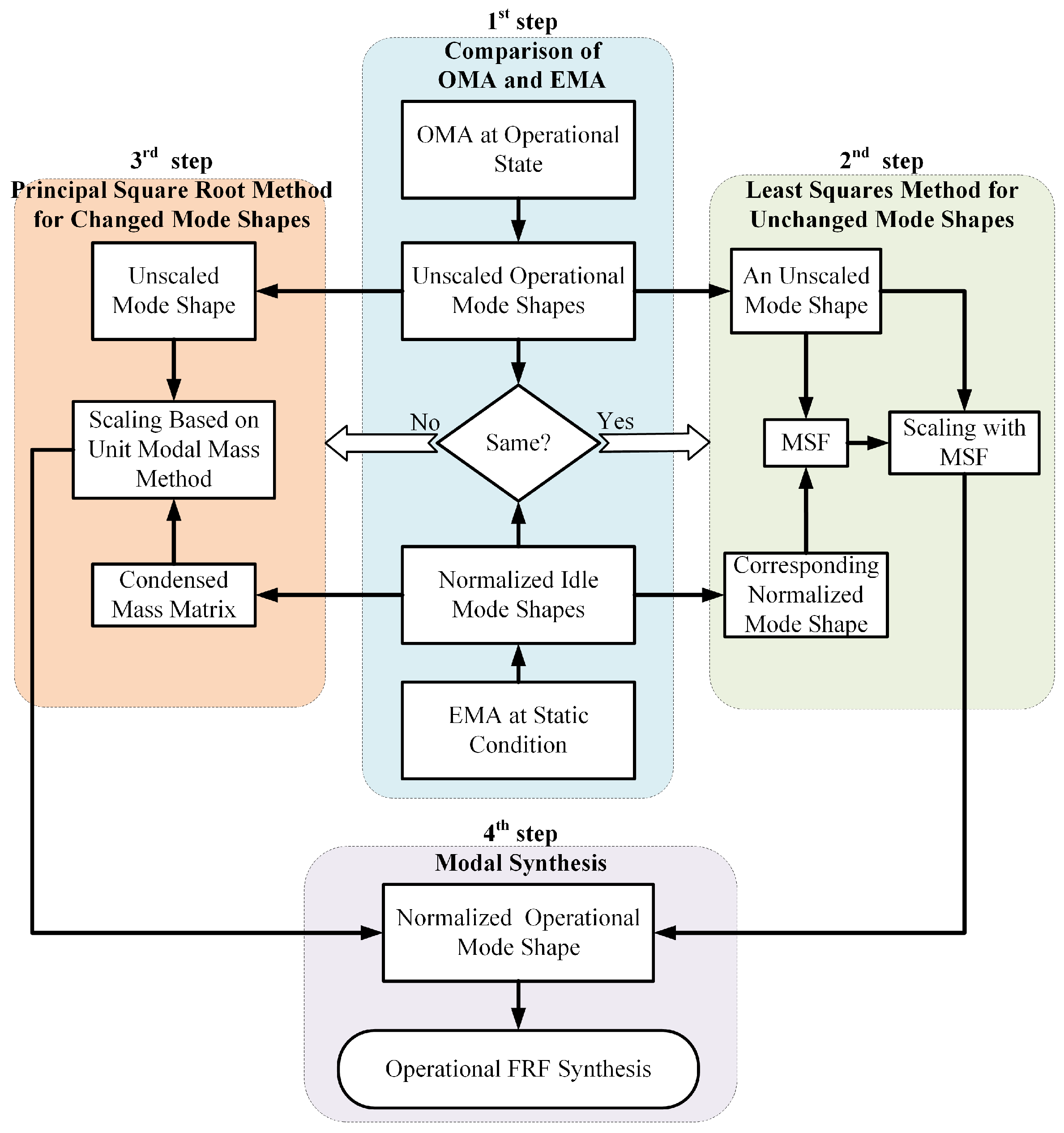
3.1. The Main Idea and Procedures

To remedy scenarios where operating mode shapes may change, a hybrid method based on EMA and OMA is proposed. Its main idea is to utilize mass information identified from EMA for operational mode shape scaling. The procedures are illustrated in Figure 1, and described as follows.

Firstly, EMA and OMA are conducted at static and operating state. According to the similarity between the mode shapes from EMA and OMA, operational mode shapes are categorized into two groups: the changed mode shapes and the unchanged ones. The modal assurance criterion (MAC) is used to compare mode shapes, which is defined as

$${\mathrm{MAC}}_{({\widehat{\mathit{\varphi }}}_e,{\mathit{\varphi }}_o)}={\displaystyle \frac{|{\widehat{\mathit{\varphi }}}_e^T{\mathit{\varphi }}_o{|}^2}{\left({\widehat{\mathit{\varphi }}}_e^T{\widehat{\mathit{\varphi }}}_e\right)\left({\mathit{\varphi }}_o^T{\mathit{\varphi }}_o\right)}},$$

(1)

where ${\mathit{\varphi }}_e$ and ${\mathit{\varphi }}_o$ represent the mode shapes from EMA and OMA, respectively, and $^$ indicates the mode shape is real and mass-normalized. In reality, operational mode shapes inevitably exhibit changes to some extent. However, unless the MAC value for a corresponding mode falls below a certain threshold, such as $\epsilon <0.7$, the operational mode shape is considered unchanged relative to the idle mode shape.

In the second step, with the help of modal scale factor (MSF) calculated as

$$\mathrm{MSF}\left({\widehat{\mathit{\varphi }}}_e,{\mathit{\varphi }}_o\right)={\displaystyle \frac{{\widehat{\mathit{\varphi }}}_e^T{\mathit{\varphi }}_o}{{{\mathit{\varphi }}_o}^T{\mathit{\varphi }}_o}},$$

(2)

the unchanged operational modes can be scaled according to corresponding modes of EMA, in the perspective of least squares; see Equation (3).

$${\widehat{\mathit{\varphi }}}_o=MSF\left({\widehat{\mathit{\varphi }}}_e,{\mathit{\varphi }}_o\right)·{\mathit{\varphi }}_o$$

(3)

The third step is specifically designed for the remarkably altered operational mode shapes. Since idle mode shapes are mass-normalized, a condensed mass matrix can be estimated. Based on the third assumption in the previous section, the condensed mass of mechanical structures is stable during operation. Then the operational mode shapes can be scaled to satisfy unit modal mass condition, which is called the principal square root method.

Finally, with a combination of ${\widehat{\mathbf{\Phi }}}_o$ via two methods, OFRF synthesis can be completed according to

$$\begin{array}{c}\hfill \mathbf{H}\left(\omega \right)=\sum _{r=1}^n{\displaystyle \frac{{\widehat{\mathit{\varphi }}}_{or}·{\widehat{\mathit{\varphi }}}_{or}^T}{-{\omega }^2+{\omega }_r^2+i2{\zeta }_r{\omega }_r\omega }},\end{array}$$

(4)

where ${\omega }_r$, ${\widehat{\mathit{\varphi }}}_{or}$ and ${\zeta }_r$ are, respectively, the modal circular frequency, mode shape and modal damping for the rth operational mode, and i is the imaginary unit.

The third step is the core element of this method, offering a novel approach to handling altered operational mode shapes. The following subsection details the principal square root method, comprising the estimation of condensed mass and its sensitivity. Moreover, this section also explains why not all operational mode shapes are scaled during this step.

3.2. The Principal Square Root Method for the Third Step

This subsection describe the theoretical basis and details for scaling-changed operational mode shapes, beginning with the estimation of the condensed mass matrix.

For an N-DOF structure, the mode problem is defined as a generalized eigenvalue problem

$$\mathbf{M}\mathbf{\Phi }\mathbf{\Lambda }+\mathbf{K}\mathbf{\Phi }=\mathbf{0},$$

(5)

where $\mathbf{M},\mathbf{K}\in {\mathbb{R}}^{N\times N}$ are symmetry matrices of mass and stiffness, and $\mathbf{\lambda },\mathbf{\Phi }$ indicate the eigenvalue and mode shape matrix. Given the inevitability of measurement incompleteness in practice, the number of measured DOFs m and estimated modes n are far fewer than the total number of DOFs and modes. This is why the mass estimated in the third step actually corresponds to the condensed system and is called the condensed mass matrix.

It can be further explained with the system equivalent reduction expansion process (SEREP) [37]. If measured DOFs and other DOFs are denoted with subscripts _m and _s, respectively, the reduction of the entire displacement vector can be expressed according to dynamic information as

$$\begin{array}{cc}\hfill \mathbf{x}& =\left[\begin{array}{c}{\mathbf{x}}_m\\ {\mathbf{x}}_s\end{array}\right]=\left[\begin{array}{c}{\widehat{\mathbf{\Phi }}}_m\\ {\widehat{\mathbf{\Phi }}}_s\end{array}\right]{\widehat{\mathbf{\Phi }}}_m^{†}{\mathbf{x}}_m=\mathbf{T}{\mathbf{x}}_m.\hfill \end{array}$$

(6)

Subsequently, the entire structure can be condensed using the transformation matrix $\mathbf{T}$ defined in the previous equation, and the initial mode problem becomes

$${\mathbf{M}}_m{\mathbf{\Phi }}_m\mathbf{\Lambda }+\mathbf{K}{\mathbf{\Phi }}_m=\mathbf{0},$$

(7)

where ${\mathbf{M}}_m={\mathbf{T}}^T\mathbf{M}\mathbf{T}$, ${\mathbf{K}}_m={\mathbf{T}}^T\mathbf{K}\mathbf{T}$.

Once $\mathbf{\Phi }$ is normalized with respect to $\mathbf{M}$, the measured mode shape matrix yield

$${\widehat{\mathbf{\Phi }}}_{\mathbf{m}}^T{\mathbf{M}}_m{\widehat{\mathbf{\Phi }}}_{\mathbf{m}}=\mathbf{I},$$

(8)

where $\mathbf{I}$ is identity matrix. With some algebraic manipulations, and replacing the subscript _m of mode shape matrix with _e, it is easy to obtain the condensed mass matrix

$${\mathbf{M}}_m={\left({\widehat{\mathbf{\Phi }}}_m{\widehat{\mathbf{\Phi }}}_m^T\right)}^{†}={\left({\widehat{\mathbf{\Phi }}}_e{\widehat{\mathbf{\Phi }}}_e^T\right)}^{†},$$

(9)

where † represents the Moore–Penrose inverse. It should be noted that, in order to use as much modal information as possible and theoretically avert the singularity of a condensed mass matrix, this paper requires $n=m$, namely ${\widehat{\mathbf{\Phi }}}_e\in {\mathbb{R}}^{m\times m}$. In this case, the Moore-Penrose inverse in Equation (9) is equivalent to a general matrix inversion.

Subsequently, the operational mode shape matrix ${\mathbf{\Phi }}_o$ will be scaled with the condensed mass. To calculate modal mass of the operating structure, the real mode shapes must first be identified from the complex complex operational mode shapes. In the absence of input signals, classical methods [38,39] for extracting real modal parameters are not applicable. This paper attempts to minimize the imaginary parts of mode shapes according to the first assumption in Section 2.

As damping effect is restricted, the phases of elements in a complex mode vector ${\mathit{\varphi }}_o$ are nearly the same, which is known as modal phase collinearity (MPC) [40]. The vector hence extends close to a straight line in the complex plane, and the mean direction can be expressed by a unit complex number as

$$w_p=[1+i·Re{\left({\mathit{\varphi }}_o\right)}^{†}Im\left({\mathit{\varphi }}_o\right)]/|1+i·Re{\left({\mathit{\varphi }}_o\right)}^{†}Im\left({\mathit{\varphi }}_o\right)|.$$

(10)

where $|*|$ denotes the absolute value. To counteract the mean phase angles of ${\mathit{\varphi }}_o$, a unitary diagonal matrix can be defined as

$$\mathbf{W}=diag\left([w_1^{*},w_2^{*},\dots ,w_m^{*}]\right).$$

(11)

The superscript * is notation of a conjugate complex number. It is obvious that ${\mathbf{\Phi }}_o\mathbf{W}$ is still a complex mode shape matrix of the operating structure. Meanwhile, the imaginary part of ${\mathbf{\Phi }}_o\mathbf{W}$ is minimized and negligible so as to obtain a real modal shape matrix

$$\tilde{\mathbf{\Phi }}=Re\left(\left[{\mathit{\varphi }}_{o1},{\mathit{\varphi }}_{o2},\dots ,{\mathit{\varphi }}_{om}\right]\mathbf{W}\right),$$

(12)

where ˜ implies real modal parameters. For unchanged mode shapes in the second step, the least squares method makes them close to real mode shapes ${\mathit{\varphi }}_e$ without the need of Equation (12).

A common method to normalize operational mode shapes is to scale each one individually. For an arbitrary mode shape ${\tilde{\mathit{\varphi }}}_o$, it can be scaled as

$${\widehat{\mathit{\varphi }}}_o={\tilde{\mathit{\varphi }}}_o·{\displaystyle \frac{1}{\sqrt{{\tilde{\mathit{\varphi }}}_o^T{\mathbf{M}}_m{\tilde{\mathit{\varphi }}}_o}}}.$$

(13)

However, it does not constrain the relation between different mode shapes. Due to errors in measurement and modal parameter identification, the operational mode shape matrix often fails to strictly satisfy the orthogonality condition with respect to the estimated condensed mass ${\mathbf{M}}_m$. The same applies to the mode shape matrix scaled through Equation (13).

To tackle this issue, some modification of ${\mathbf{M}}_m$ or ${\tilde{\mathbf{\Phi }}}_o$ in the scaling process is unavoidable. Based on assumption (3) in Section 2, the results from OMA are less precise than those from EMA; thus, ${\tilde{\mathbf{\Phi }}}_o$ should be the one to be modified. Mathematically, the problem becomes to find the nearest matrix ${\widehat{\mathbf{\Phi }}}_o$ to the initial unscaled ${\tilde{\mathit{\varphi }}}_o$, and simultaneously meets the unit modal mass condition, namely

$$\begin{array}{cc}\hfill {∥{\mathbf{M}}_m^{{\displaystyle \frac{1}{2}}}({\tilde{\mathbf{\Phi }}}_o-{\widehat{\mathbf{\Phi }}}_o)∥}_F& =min\left\{{∥{\mathbf{M}}_m^{{\displaystyle \frac{1}{2}}}({\tilde{\mathbf{\Phi }}}_o-\mathbf{Q})∥}_F\right\},\hfill \\ \hfill s.t.{\mathbf{Q}}^{\mathbf{T}}{\mathbf{M}}_m\mathbf{Q}& =\mathbf{I},\mathbf{Q}\in {\mathbb{R}}^{n\times n},\hfill \end{array}$$

(14)

where ${∥·∥}_F$ denotes Frobenius norm. ${\mathbf{M}}_m^{{\displaystyle \frac{1}{2}}}$ acts as a weight matrix in view of kinetic energy. Appendix A obtains the solution for the optimization problem as

$${\widehat{\mathbf{\Phi }}}_o={\tilde{\mathbf{\Phi }}}_o·{\left({\tilde{\mathbf{\Phi }}}_o^T{\mathbf{M}}_m{\tilde{\mathbf{\Phi }}}_o\right)}^{-{\displaystyle \frac{1}{2}}}.$$

(15)

As mentioned, ${\tilde{\mathbf{\Phi }}}_o^T{\mathbf{M}}_m{\tilde{\mathbf{\Phi }}}_o$ may not be diagonal, and the notation ${()}^{\frac{1}{2}}$ implies the principal square root of a matrix. The principal square root of a matrix can be seen as a matrix function defined on the spectrum of the independent variable matrix. Since the condensed matrix estimated using real mode shapes is positive definite and so is the modal mass matrix, the principal square root matrix exits and is uniquely positive definite. The algorithm and relevant theory for principal square root can be found in Ref [41].

Compared with Equation (13), which uses the square root of a scalar, Equation (15) exploits the square root of the modal mass matrix to scale and modify the operational mode shape matrix simultaneously. This guarantees the orthogonality of the scaled mode shapes.

The direct method of FEM model updating uses a formula similar to Equation (15) [42]. The only difference is the number of mode shapes to be modified. The third step actually requires scaling only the altered mode shapes. If all m operational mode shapes are scaled using Equation (15), as in model updating, there is a risk that the condition number of the principal square root of the modal mass matrix may become too large, making matrix inversion unstable. Reducing the number of mode shapes to scale decreases the dimension of the modal mass matrix, which generally enhances numerical stability.

3.3. The Stability of Condensed Mass and Countermeasures

The operational mode shapes can be scaled using the condensed mass with the principal square root method. Nevertheless, since the modal shape matrix may vary as the mechanical equipment starts operating, theoretically, the corresponding condensed mass may differ from the estimated one. This subsection discusses the stability of the condensed mass matrix as a further theoretical supplement and presents corresponding solutions.

Aenlle et al. [32] studied the effect of mass error when using FEM to scale operational mode shapes. They proved that some changes are permissible and the extent of these changes is crucial. Therefore, it is essential to study the sensitivity of the condensed mass to variations in the mode shapes. This sensitivity analysis ensures the reliability of the scaling process in previous subsection and the accuracy of the resulting scaled mode shapes.

For clarity, the condensed mass is defined as a function

$${\mathbf{M}}_m=\mathbf{F}\left({\widehat{\mathbf{\Phi }}}_m\right)={\left({\widehat{\mathbf{\Phi }}}_m{\widehat{\mathbf{\Phi }}}_m^T\right)}^{-1}.$$

(16)

The objective is to find the maximum relative change in $\mathbf{F}\left({\widehat{\mathbf{\Phi }}}_m\right)$ caused by an arbitrary relative change in ${\widehat{\mathbf{\Phi }}}_o$. Mathematically, sensitivity is actually a condition number problem of a matrix function, based on the norm of Fréchet derivative, if it exists [41]. For $\mathbf{F}\left({\widehat{\mathbf{\Phi }}}_m\right)$, its sensitivity can be computed as

$$cond=\underset{\Delta {\widehat{\mathbf{\Phi }}}_m\ne 0}{max}{\displaystyle \frac{∥\mathbf{L}({\widehat{\mathbf{\Phi }}}_m,\Delta {\widehat{\mathbf{\Phi }}}_m)∥}{∥\Delta {\widehat{\mathbf{\Phi }}}_m∥}}·{\displaystyle \frac{∥{\widehat{\mathbf{\Phi }}}_m∥}{∥\mathbf{F}\left({\widehat{\mathbf{\Phi }}}_m\right)∥}},$$

(17)

where $\Delta {\widehat{\mathbf{\Phi }}}_m$ represents variation of mode shape matrix, and $\mathbf{L}$ is the notation of Fréchet derivative. The norm can be any matrix norm in principle, but in the following text it is designated as the spectral norm.

As to matrix function Equation (16), the Fréchet derivative can be derived using the Gâteaux derivative as

$$\begin{array}{cc}\hfill \mathbf{L}({\widehat{\mathbf{\Phi }}}_m,\Delta {\widehat{\mathbf{\Phi }}}_m)& =\underset{t\to 0}{lim}{\displaystyle \frac{\mathbf{F}({\widehat{\mathbf{\Phi }}}_m+t\Delta {\widehat{\mathbf{\Phi }}}_m)-\mathbf{F}\left({\widehat{\mathbf{\Phi }}}_m\right)}{t}}\hfill \\ \hfill & ={\left({\widehat{\mathbf{\Phi }}}_m{\widehat{\mathbf{\Phi }}}_m^T\right)}^{-1}·(\Delta {\widehat{\mathbf{\Phi }}}_m·{\widehat{\mathbf{\Phi }}}_m^T+{\widehat{\mathbf{\Phi }}}_m^T·\Delta {\widehat{\mathbf{\Phi }}}_m^T)·{\left({\widehat{\mathbf{\Phi }}}_m{\widehat{\mathbf{\Phi }}}_m^T\right)}^{-1}\hfill \end{array}$$

(18)

Substitute Equations (16) and (18) into (17), and then we have

$$\begin{array}{cc}\hfill cond& =\underset{\Delta {\widehat{\mathbf{\Phi }}}_m\ne 0}{max}{\displaystyle \frac{{∥{\mathbf{M}}_m\Delta {\widehat{\mathbf{\Phi }}}_m{\widehat{\mathbf{\Phi }}}_m^{-1}+{\widehat{\mathbf{\Phi }}}_m^{-T}\Delta {\widehat{\mathbf{\Phi }}}_m^T{\mathbf{M}}_m∥}_2}{{∥\Delta {\widehat{\mathbf{\Phi }}}_m∥}_2}}·{\displaystyle \frac{{∥{\widehat{\mathbf{\Phi }}}_m∥}_2}{{∥{\mathbf{M}}_m∥}_2}}\hfill \\ \hfill & =2{∥{\widehat{\mathbf{\Phi }}}_m∥}_2{∥{\widehat{\mathbf{\Phi }}}_m^{-1}∥}_2=2\kappa .\hfill \end{array}$$

(19)

where $\kappa$ is the condition number of mode shape matrix ${\widehat{\mathbf{\Phi }}}_m$ for matrix inversion.

Therefore the matrix ${\mathbf{M}}_m$ estimated with EMA is applicable to scale operational modes, when the value $\kappa$ and modification of ${\widehat{\mathbf{\Phi }}}_m$ are both limited. Since the modes used for the condensed mass estimation are the first several modes of the structure, as stated in assumption (2) in Section 2, each measured mode shape is sufficiently distinct from the others, leading to a quite small $\kappa$. It is possible that prominent differences may appear locally in a few operational mode shapes [28]. When these modes are much fewer than others, which fortunately often conforms to reality, the estimated mass matrix is still believed to be accurate enough. Moreover, it may be the only basis for these modes to be scaled, if an exact FEM model is not available.

In practice, however, there is a possibility that $\kappa$ is large, especially when sensors are not arranged properly or the the number of measured DOFs are too limited to clearly distinguish some idle mode shapes. Of course, the corresponding solution is to rearrange or add more sensors. If the changed operational mode shapes result in a small $\kappa$ for ${\mathbf{\Phi }}_o$, which includes all m operational mode shapes, there is an alternative method. It reverses the sequence of square root operation and matrix inversion, as shown in

$${\widehat{\mathbf{\Phi }}}_o={\mathbf{\Phi }}_o·{\left[{{\mathbf{\Phi }}_o}^{-1}·\left({\widehat{\mathbf{\Phi }}}_m{\widehat{\mathbf{\Phi }}}_m^{\mathbf{T}}\right)·{{\mathbf{\Phi }}_o}^{-T}\right]}^{{\displaystyle \frac{1}{2}}}.$$

(20)

This approach evades successive matrix inversions but involves ${\mathbf{\Phi }}_o$ in the inversion process. So the inversion stability of ${\mathbf{\Phi }}_o$ must be guaranteed.

3.4. Practical Implementation

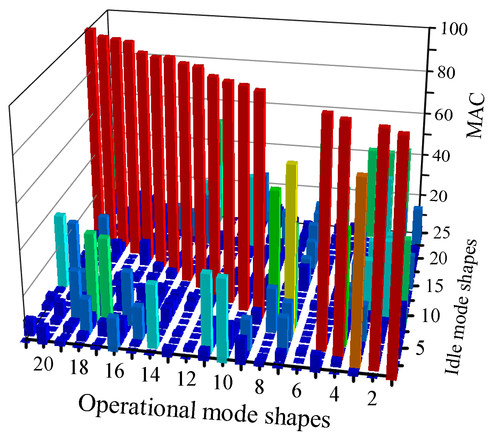
• The number of measured DOFs m should be sufficient to reduce the likelihood that MAC matrix for different idle mode shapes has large elements, which may result in a high $\kappa$. The exact number should be determined comprehensively considering test demands and the complexity of the structure.
• Modes beyond the frequency band of interest in OFRF are needed. They will supplement upper and low residues beyond frequency band and thus promote estimation accuracy of OFRFs.
• The proposed method is derived based on normal modes. For structures with high damping, the accuracy may decrease.
• All approaches that improve EMA precision can benefit the identification of OFRFs. For instance, selecting appropriate frequencies as boundaries during EMA, and checking for reciprocity. FRFs that significantly violate reciprocity would affect the estimation of modal shape and ultimately cause trouble in the normalization of operational modes.

4. Case Studies

To validate the proposed method, we employ a numerical model and an experimental case, accounting for noise and incomplete measurement. The first example involves a continuous structure modeled using FEM, where artificial perturbations can be introduced easily. The second case illustrates the application of the proposed method in a real-world scenario.

The following process simulates operating conditions by modifying parameters related to stiffness. In other words, two sets of different structural parameters are used: one for the structure’s property in a static state, referred to as the original structure, and the other for the operating state, referred to as the targeted structure, as used in Ref. [36]. This approach allows us to bring in arbitrary changes, including geometry parameters and boundary conditions, making the modal parameters’ variations sufficient to test the capability of the proposed method. Additionally, it is convenient to obtain the exact FRFs to evaluate the precision of the estimated OFRFs.

The proposed method is verified as follows. Firstly, the estimator commercially known as POLYMAX [43] is applied on contaminated FRFs of the original systems during the EMA process. Next, stiffness matrices are altered to obtain the targeted systems, with perturbations introduced to study sensitivity of condensed mass, and OMA is performed. With the proposed method, FRFs for the target system are identified and compared with the exact ones. As the main focus of this paper is scaling, details in EMA and OMA are not included in this section.

4.1. Simulation Example

Figure 2a displays the original structure. Three beams connect to a square steel plate and intersect at point P. A lumped mass is attached to the plate and point P vertically with two springs. A coordinate system is set at point O, whose x-axis directs point A and y-axis extends towards point D. Geometric and dynamic parameters are listed in

Table 1. Geometric and dynamic parameters of original system.

Items	Original System	Unit
Coordinate of P	(300, 500, 300)	mm
Side length of plate	1000	mm
Thickness of plate	5	mm
Section diameter of beam	6	mm
Material density	$7.85\times {10}^{-6}$	kg/mm3
Elasticity modulus	210	GPa
Poisson’s ratio	0.3	—
Mass of mass point	1	kg
Stiffness of spring	0.5, 100, 100	${10}^3$N/mm
Damping of spring	5, 100, 100	N·s/mm
Shell element size	$10\times 10$	mm
Number of elements per beam	1	—

, where stiffness and damping values are arranged sequentially along the directions of the x-, y-, and z-axis of the coordinate system. Triangles on the edges indicate constraints.

In the target structure, shown in Figure 2b, the elasticity modulus of one beam and three-quarters of the plate, highlighted in red color, is changed to 185 GPa. The stiffness and damping of the two springs are changed to 1000, 80,000, 80,000 N/mm and 10, 80, 80 N·s/mm, respectively. More details of the models can be found in Appendix B.

The dynamic responses of the normal DOFs at 16 points, evenly distributed along the edge of the plate, and the three translational DOFs of the lumped mass are considered. Accordingly, 19 mode shapes are required for condensed mass estimation. Nastran is utilized for FEM computation, as well as the following analyses. Mode shapes of the original structure are mass-normalized, representing “static” mode shapes. In contrast, mode shapes of the target structure are scaled so that the largest element of each mode shape vector is one, indicating the “operational” mode shapes.

Validations begins with a brief analysis without considering errors in the modal parameters, showing the necessity of the principal square root method. The proposed method assumes that the estimated condensed mass is stable enough to scale operational mode shapes, despite the presence of measurement errors and big variations of modal shapes. Thus, to verify the stability of the method, intentional perturbations are introduced to the mass matrix in the second case, in addition to contaminated data and incomplete measurements.

Modal parameters of both the original and target structures can be computed with FEM models, when errors in EMA and OMA are ignored. Figure 3 illustrates the MAC matrix between the mode shapes of the two structures, showing that there are no idle mode shapes similar to the sixth, seventh, and eighth operational mode shapes, and even 25 static modes are involved. The variations in natural frequencies between the original and targeted structures, which are not so crucial for the proposed method, can be seen in

Table A2. Comparison between the natural frequencies of the original and targeted structure in the first case of the simulation example (unit: Hz).

The Original Structure	The Targeted Structure
11.3829	10.8636
19.7494	18.7843
25.0262	19.6450
36.8577	23.6460
43.3347	35.4094
52.3165	42.5321
53.6780	50.3279
57.9709	52.1611
71.4442	55.4953
83.3543	68.4422
89.5122	79.8620
99.1503	85.4602
102.9488	93.4075
125.8974	98.0684
132.2300	119.3317
138.6529	125.5628
152.4326	132.6460
163.3064	146.4351
168.6131	154.5092
188.2306	161.2042
218.2984	178.4255
223.2421	209.2524
229.6832	213.1208

in Appendix C.

Figure 4 presents the identified OFRF between 10 and 220 Hz, with the normal DOF at point A as the input, and vertical acceleration responses of point B, C, D and the lumped mass as the outputs. The three output DOFs on plate are chosen to represent DOFs near the load, close to constraints and far away from the input DOF, respectively. The FRF amplitudes are illustrated using dB values referenced to 1, with acceleration and force units being mm/s² and N, respectively. If the operational mode shapes are replaced with idle mode shapes, OFRFs are estimated as shown by the blue line and labeled as “Idle mode shapes method” in the legend. The results of the hybrid method, which scale the sixth to eighth mode shapes using the principal square root method, are depicted with the red line with square markers.

It can be observed that idle mode shapes, in combination with natural frequencies of the target structure, provide high accuracy for identified OFRFs, except in the frequency range between 35 and 55 Hz, which corresponds to the sixth to eighth operational modes. Especially for the OFRF at the lumped mass along z direction in Figure 4d, a peak disappears compared with the exact FRF. The hybrid method utilizes the least squares method to scale most operational mode shapes according to idle mode shapes, ensuring precision for OFRFs in most frequency points. Simultaneously, the principal square root method effectively addresses the sixth to eighth operational modes, reducing errors in OFRFs notably compared to using idle mode shapes directly. This example demonstrated that the principal square method is applicable in OFRF estimation, and is necessary when the mass-change method and FEM method are not feasible due to some actual conditions.

To verify the stability of the proposed method, noise and errors are considered. Transient response analyses are performed on the original structure to simulate impact testing for CFRF measurement. An impulse signal, acting as a hammer impact force, is applied in sequence at four corners of the plate along the z direction. The time step is ${10}^{-3}$ s and the total duration is 5 s for each computation. Normal accelerations of the 16 points and translational accelerations of the lumped mass are calculated using solution sequence SOL 109 of Nastran. CFRFs are then obtained through the H₁ estimator, with an exponential window applied to act as artificial damping. Errors from the transient analysis and H₁ estimator are treated as noise.

Based on the estimated CFRF, 19 modes are identified in the frequency band of 6–172 Hz using POLYMAX in the EMA process. Figure 5 shows CFRFs and the modal synthesis results. The artificial damping is eliminated for the comparison with theoretical FRFs of the target structure. From Figure 5b, noise in CFRF at point C is relatively higher. This is because point C can hardly be excited for its proximity to the constrained DOFs. CFRFs at this point are not eliminated in EMA. Despite this, the synthesized curves are accurate and almost coincide with the exact FRFs at other DOFs in Figure 5, except for the peak near 43 Hz at sub-figure (c). This error in idle mode shape is retained to examine the proposed method.

Additionally, perturbations in mass are introduced in target structure. The geometric parameters of components highlighted in red color are also changed. Specifically, the section diameter of the beam is modified to 10 mm, and the thickness of the three-quarter plate is adjusted to 6 mm. As a result, the total mass is thus increased by 6.3 kg, or $15\%$ of the original structure’s mass, which undoubtedly affects the condensed mass. The variations in natural frequencies become more notable than previous case, as seen in

Table A3. Comparison between the natural frequencies identified from EMA and OMA in the second case of the simulation example (unit: Hz).

The Original Structure	The Targeted Structure
11.3825	12.5928
19.7554	21.4307
25.0330	27.2876
36.8915	39.8742
43.6217	57.7508
52.6610	62.9120
53.7115	77.2842
57.9793	82.8056
71.4567	96.0678
83.3827	97.8849
89.4947	110.8344
99.1247	112.9849
102.9327	137.5893
125.8468	144.9645
132.2340	151.1522
138.5813	162.2044
152.3783	179.5252
163.3391	184.6468
168.6119	207.0478

in Appendix C.

Before OMA, a stochastic simulation is performed. Forces explicitly defined with irrelevant white noises are applied simultaneously at four corners along the normal direction, and responses of the same DOFs as in EMA are computed, with a time step of ${10}^{-3}$ s. SOL 112 is used for simulation with modes beyond 6000 Hz excluded. Numerical errors are considered as noise. During OMA process, 19 operational modes are estimated. The first operational mode shape is selected to match the first idle mode shape.

The MAC matrix between operational and idle mode shapes can be seen in Figure 6. Variations in mode shapes are more pronounced at the fifth and ninth mode than in the previous example, and significant changes are also evident in the sixth and eighth modes. The corresponding natural frequencies are 57.8 Hz, 62.9 Hz, 82.8 Hz and 96.1 Hz. The threshold value $\epsilon$ is set to 0.7, so that only those four mode shapes are deemed changed. Therefore, those four mode shapes are normalized with Equation (20), whereas other operational mode shapes are scaled via MSF. Meanwhile, the estimation method using idle mode shapes directly is also conducted. The frequency band for synthesizing OFRFs is defined between 10 and 220 Hz.

Identified OFRFs with the input DOF in the vertical direction of point A, and the output DOFs in the vertical directions at point B, C, D and the lumped mass, are shown in Figure 7. The figure reveals that deviations between OFRFs synthesized with idle mode shapes and the exact FRFs cannot be eliminated at the four frequencies of 57.8, 62.9, 82.9 and 96.1 Hz in each sub-figure. In comparison, results of the hybrid method align with the theoretical FRFs at these four frequency points, owing to the principal square root method. Furthermore, as shown in Figure 7c, the hybrid method outperforms the idle mode shapes method around the peak at 77.3 Hz. But in fact, the corresponding MAC value is as high as 0.955 and the operational mode shape is scaled to just match the static one in hybrid method, indicating that this phenomenon can only be attributed to the variation of the adjacent mode shapes. At other frequency points, the hybrid method maintains high precision, except for peaks at 110 Hz in Figure 7b and c, where the idle mode shapes method also gives a larger value.

OFRFs at the same DOFs but excited at point O are depicted in Figure 8. Just like the previous results, the proposed method performs quite well, especially around the frequencies dominated by the changed mode shapes compared to the idle mode shapes method. Moreover, these OFRFs around 110 Hz in Figure 8b and c are extremely accurate.

The errors at 110 Hz in Figure 7 actually result from deviations in the operational mode shape. Figure 9 compares the estimated operational mode shape at 110 Hz with the theoretical one from FEM. In Figure 9a, the dotted line indicates the undeformed plate, while the solid line depicts the modal displacement of the twelve DOFs in OMA. Figure 9b displays the FEM result with a contour map, where the modal displacements of the nodes are color-coded according to the color bar. Point A is expected to be a nodal point according to FEM, as shown in Figure 9b, but the OMA result clearly contradicts this.

Table 2. The mode shapes corresponding to OFRFs at 110 Hz.

DOF	The OMA Result	The Exact Mode Shape
A	0.0525 − 0.1887i	−0.0623
B	0.1104 − 0.0493i	0.0705
C	−0.0585 + 0.0010i	−0.0590
D	1	1
O	0.4604 + 0.0466i	0.4771
The lumped mass	0.1796 − 0.0151i	0.1676

lists the mode shape elements related to the OFRFs, where the element corresponding to point D is set to 1 for ease of comparison. The element for point A in estimated operational mode shape has a substantial imaginary value that cannot be neglected, whereas other elements are close to the theoretical values. This discrepancy might stem from numerical error in the stochastic simulation or OMA.

In summary, this subsection proves the applicability and high stability of the hybrid method, even when noise and errors in EMA, as well as perturbations in mass, are taken into consideration. However, precision of operational modal parameters should be examined, such as unreasonable damping effects.

4.2. Experimental Example

This subsection will describe our test of the proposed method in the real world. Since estimated static modal parameters may vary over time, between testers, and with the CFRFs used, condensed mass changes accordingly. The following analysis compares the resulting OFRFs to study the feasibility and stability of the hybrid method. Similar to the simulation examples, dynamic attributes are modified with a new constraint to represent the operating condition, making it easy and reliable to obtain the exact “operational” FRFs with the H₁ estimator.

The structure under analysis is illustrate in Figure 10a. The steel structure has a 500 mm × 500 mm × 5 mm plate on the top, supported by only three legs. Twelve acceleration sensors are distributed evenly along the edge of the surface, with a tri-axial sensor located at the unsupported corner. Among the measured points, points A and C are free, while points B and D are positioned near beams. During the EMA process, only two legs are fixed, whereas during the OMA process, the other leg is also pressed onto the ground with a bolt to increase the system stiffness, as shown in Figure 10b. This change greatly alters the dynamic characteristics, which is reflected in the comparison of natural frequencies under the two boundary conditions in

Table A4. Comparison between the natural frequencies identified from EMA and OMA in the experimental example (unit: Hz).

The Original Structure	The Targeted Structure
56.2318	57.9509
64.9327	64.2205
109.6792	115.5228
154.3924	164.5742
201.9135	223.7241
232.8787	237.3319
260.2597	263.0481
284.6582	310.9808
319.4749	329.2040
333.7813	350.3971
372.3621	361.5300
405.0700	388.7280
420.2550	412.9673
443.1399	436.9488

in Appendix C. An exciter is mounted on the horizontal beam throughout the experiment process and provides white noise as the input load in OMA. Taking the normal acceleration of free corner as the target, OFRFs with inputs from points A, B, C and D in the normal direction are identified. This subsection also uses dB values referenced to 1 to evaluate the FRF magnitudes, but the unit for acceleration is changed to g, causing the magnitude values to decrease sharply compared with the previous cases.

Using different combinations of CFRFs in EMA results in different mode shapes, leading to two distinct modal synthesis outcomes, A and B, as illustrated in Figure 11. The main differences can be observed at two peaks around 50 Hz in sub-figures (a) and (d), which are determined by the first two modes. Additionally, the peak height at 285 Hz in sub-figure (a) varies. Consequently, the condensed mass matrices identified by the two EMA results also differ. Furthermore, from sub-figure (c) and the phase map in sub-figure (a), a mode at approximately 356 Hz is not identified. Sub-figure (b) illustrates that the error in the last mode shape from both EMAs is considerable. Therefore, the condensed mass matrices determined through the two EMA results both deviates from the exact value.

The MAC matrices between operational mode shapes and the two sets of idle mode shapes are shown in Figure 12. The threshold $\epsilon$ is set to 0.8. Only four modes, namely the first, third, fourth, and fifth operational mode shapes, remain unchanged compared with idle mode shapes A. Figure 12b demonstrates that the first five operational mode shapes are all unchanged in comparison with idle mode shapes B, which also implies the two idle mode shapes differ. Thereby, most operational mode shapes must be scaled with the principal square root method, whose stability is to be verified.

The OFRFs identified using the hybrid method and modal synthesis with idle mode shapes directly are compared with CFRFs through the H₁ estimator in Figure 13 and Figure 14. The former figure corresponds to idle mode shapes A, and the latter to idle mode shapes B. The analysis focuses mainly on the frequency range of the OFRFs dominated by the changed operational mode shapes. Thus, the emphasis is placed on the frequency band containing the 6th to 14th peaks, or from 230 to 450 Hz, in both figures, as well as the 2nd peak in Figure 13.

Regarding the frequency range from 230 to 450 Hz, both figures exhibit the high accuracy of the hybrid method in terms of peak heights. In contrast, the idle mode shapes method does not perform well, particularly in the range from 300 to 430 Hz. The last peak is an exception, where the hybrid method fails to identify the peak value accurately. This discrepancy derives from the prominent error in the last idle mode shape from EMA, as shown in Figure 11b.

Moreover, despite the condensed mass used in the two figures not being identical, the hybrid method produces similar results, which demonstrates the stability. The differences are concentrated in the regions between peaks, such as 175–225 Hz in sub-figure (a) and 200–225 Hz in sub-figure (b) of the both figures. Fortunately, these areas are often not critical in practical application.

The height of the second peak of the identified OFRF with idle mode shapes A serves as another good indicator of stability. The operational mode shape changes compared to the corresponding idle mode shape A, but remains consistent with corresponding idle mode shape B. When idle mode shapes are directly used for synthesizing OFRFs, the second peaks of OFRFs in Figure 13a,b,d deviate from the exact FRFs evidently. With the principal square root method, however, the identified OFRFs improve dramatically, achieving a precision comparable to those in Figure 14, where the second mode shape is scaled using least squares method.

Another example is the comparison between Figure 13a and Figure 14a at 311 Hz. The idle mode shapes method behaves quite differently in the two figures at that peak, revealing that the corresponding idle mode shape A and B are distinct. Even so, the condensed mass is stable enough for scaling in principal square root method, so that accurate identified OFRFs can be seen in both figures.

In conclusion, the proposed method is feasible in application. Uncertainty in measurement and error in EMA are considered, though, the hybrid method still demonstrates high accuracy and stability.

5. Conclusions

This work presents a hybrid method to identify operational FRF. EMA at the static state is introduced as a supplement to operational modal information for OFRF identification.

The hybrid method combines two approaches according to whether operational changes occur in idle mode shapes. Unchanged operational mode shapes are scaled with the least squares method, while changed ones are normalized though the principal square root method, which is the main focus of this paper. EMA at the static state is utilized in the principal square root method to estimate the condensed mass or its inverse matrix, which is then used to normalize the operational modes from OMA. These tow steps allow for the calculation of the OFRFs.

Stability is emphasized in the principal square root method, including the stability of the condensed mass matrix and the inversion computation. The condition number for the estimated condensed mass with respect to variations of mode shapes is investigated. Two methods are proposed to tackle the possible instability in matrix inversion.

The precision of the proposed method is demonstrated through two examples. Noises in measurement, disturbances in mass and incomplete measurements are considered in the simulation example. A measurement example, concentrated in stability of the proposed method, compares the results with different EMA results. In conclusion, the proposed method is feasible and provide adequate accuracy in those examples, offering a new approach for OFRF estimation.

The main source of error may be the precision of EMA and OMA, especially the latter one, as EMA techniques are usually more reliable. This article involve no issues in modal parameter estimation, such as spurious modes, and takes it for granted that the mode shapes are acceptable.

Lastly, it should be clarified that there are also limitations to this hybrid method, corresponding to the assumptions outlined in Section 2. Since the principal square root method is based on real mode shapes, high damping effects are not considered and may require further study. Applying this method to OFRFs in high-frequency zone may also be challenging due to difficulties in identifying modal parameters and numerical issues in the principal square root method. Additionally, changes in the position or pose of sub-structures are not considered in the operating state, making the proposed method unsuitable for the gesture-dependent OFRFs of robots.

References

1. Pradhan, S.; Modak, S. A method for damping matrix identification using frequency response data. Mech. Syst. Signal Process. 2012, 33, 69–82. [Google Scholar] [CrossRef]
2. Lin, R.; Zhu, J. Model updating of damped structures using FRF data. Mech. Syst. Signal Process. 2006, 20, 2200–2218. [Google Scholar] [CrossRef]
3. Niu, Z. Frequency response-based structural damage detection using Gibbs sampler. J. Sound Vib. 2020, 470, 115160. [Google Scholar] [CrossRef]
4. Zhang, Q.; Hou, J.; Duan, Z.; Jankowski, Ł.; Hu, X. Road Roughness Estimation Based on the Vehicle Frequency Response Function. Actuators 2021, 10, 89. [Google Scholar] [CrossRef]
5. Song, J.H.; Lee, E.T.; Eun, H.C. Expansion of incomplete frequency response functions and prediction of unknown input forces. Arch. Appl. Mech. 2021, 91, 1055–1066. [Google Scholar] [CrossRef]
6. Zhao, T.; Liu, X.; Li, C.; Hou, H.; Wang, D.; Cao, Y. Electric Vehicle Interior Noise Contribution Analysis. In Proceedings of the SAE 2016 World Congress and Exhibition, Detroit, Michigan, 12–14 April 2016. [Google Scholar] [CrossRef]
7. van der Seijs, M.V.; de Klerk, D.; Rixen, D.J. General framework for transfer path analysis: History, theory and classification of techniques. Mech. Syst. Signal Process. 2016, 68–69, 217–244. [Google Scholar] [CrossRef]
8. Ocepek, D.; Vrtač, T.; Čepon, G.; Boltežar, M. Estimation of the frequency response functions for operational assemblies using independent source characterization. Mech. Syst. Signal Process. 2023, 182, 109542. [Google Scholar] [CrossRef]
9. Carne, T.G.; James, G.H. The inception of OMA in the development of modal testing technology for wind turbines. Mech. Syst. Signal Process. 2010, 24, 1213–1226. [Google Scholar] [CrossRef]
10. Li, B.; Luo, B.; Mao, X.; Cai, H.; Peng, F.; Liu, H. A new approach to identifying the dynamic behavior of CNC machine tools with respect to different worktable feed speeds. Int. J. Mach. Tools Manuf. 2013, 72, 73–84. [Google Scholar] [CrossRef]
11. Özşahin, O.; Budak, E.; Özgüven, H. Identification of bearing dynamics under operational conditions for chatter stability prediction in high speed machining operations. Precis. Eng. 2015, 42, 53–65. [Google Scholar] [CrossRef]
12. Grossi, N.; Sallese, L.; Montevecchi, F.; Scippa, A.; Campatelli, G. Speed-varying Machine Tool Dynamics Identification Through Chatter Detection and Receptance Coupling. In Proceedings of the 5th CIRP Global Web Conference—Research and Innovation for Future Production (CIRPe 2016), Patras, Greece, 4–6 October 2016; Volume 55, pp. 77–82. [Google Scholar] [CrossRef]
13. Deng, K.; Gao, D.; Zhao, C.; Lu, Y. Prediction of in-process frequency response function and chatter stability considering pose and feedrate in robotic milling. Robot. Comput.-Integr. Manuf. 2023, 82, 102548. [Google Scholar] [CrossRef]
14. Mohammadi, Y.; Ahmadi, K. In-Process Frequency Response Function Measurement for Robotic Milling. Exp. Tech. 2023, 47, 797–816. [Google Scholar] [CrossRef]
15. Karlsson, F.; Persson, A. Modelling Non-Linear Dynamics of Rubber Bushings-Parameter Identification and Validation. Master’s Thesis, Lund University, Lund, Sweden, 2003. [Google Scholar]
16. Kindt, P.; Sas, P.; Desmet, W. Measurement and analysis of rolling tire vibrations. Opt. Lasers Eng. 2009, 47, 443–453. [Google Scholar] [CrossRef]
17. Rocca, G.; Díaz, G.; Middelberg, J.; Kindt, P.; Peeters, B. Experimental Characterization of the Dynamic Behaviour of Tires in Static and Rolling Conditions. In Proceedings of the 18th International Congress on Sound & Vibration, Janeiro, Brazil, 10–14 July 2011. [Google Scholar]
18. Gonzalez Diaz, C.; Kindt, P.; Middelberg, J.; Vercammen, S.; Thiry, C.; Close, R.; Leyssens, J. Dynamic behaviour of a rolling tyre: Experimental and numerical analyses. J. Sound Vib. 2016, 364, 147–164. [Google Scholar] [CrossRef]
19. De Sitter, G.; Devriendt, C.; Guillaume, P.; Pruyt, E. Operational transfer path analysis. Mech. Syst. Signal Process. 2010, 24, 416–431. [Google Scholar] [CrossRef]
20. Coppotelli, G. On the estimate of the FRFs from operational data. Mech. Syst. Signal Process. 2009, 23, 288–299. [Google Scholar] [CrossRef]
21. Behnam, M.R.; Khatibi, M.M.; Malekjafarian, A. An accurate estimation of frequency response functions in output-only measurements. Arch. Appl. Mech. 2018, 88, 837–853. [Google Scholar] [CrossRef]
22. Peeters, B.; De Roeck, G. Stochastic system identification for operational modal analysis: A review. J. Dyn. Syst. Meas. Control Trans. Asme 2001, 123, 659–667. [Google Scholar] [CrossRef]
23. Reynders, E. System Identification Methods for (Operational) Modal Analysis: Review and Comparison. Arch. Comput. Methods Eng. 2012, 19, 51–124. [Google Scholar] [CrossRef]
24. Brincker, R.; Kirkegaard, P.H. Special issue on Operational Modal Analysis. Mech. Syst. Signal Process. 2010, 24, 1209–1212. [Google Scholar] [CrossRef]
25. Parloo, E.; Verboven, P.; Guillaume, P.; Van Overmeire, M. Sensitivity-based operational mode shape normalisation. Mech. Syst. Signal Process. 2002, 16, 757–767. [Google Scholar] [CrossRef]
26. López-Aenlle, M.; Fernández, P.; Brincker, R.; Fernández-Canteli, A. Scaling-factor estimation using an optimized mass-change strategy. Mech. Syst. Signal Process. 2010, 24, 1260–1273. [Google Scholar] [CrossRef]
27. Khatibi, M.; Ashory, M.; Malekjafarian, A.; Brincker, R. Mass-stiffness change method for scaling of operational mode shapes. Mech. Syst. Signal Process. 2012, 26, 34–59. [Google Scholar] [CrossRef]
28. Massa, F.; Tison, T.; Lallemand, B.; Cazier, O. Structural modal reanalysis methods using homotopy perturbation and projection techniques. Comput. Methods Appl. Mech. Eng. 2011, 200, 2971–2982. [Google Scholar] [CrossRef]
29. Bernal, D. Modal Scaling from Known Mass Perturbations. J. Eng. Mech. 2004, 130, 1083–1088. [Google Scholar] [CrossRef]
30. Bernal, D. A receptance based formulation for modal scaling using mass perturbations. Mech. Syst. Signal Process. 2011, 25, 621–629. [Google Scholar] [CrossRef]
31. López-Aenlle, M.; Brincker, R.; Pelayo, F.; Canteli, A. On exact and approximated formulations for scaling-mode shapes in operational modal analysis by mass and stiffness change. J. Sound Vib. 2012, 331, 622–637. [Google Scholar] [CrossRef]
32. Aenlle, M.; Brincker, R. Modal scaling in operational modal analysis using a finite element model. Int. J. Mech. Sci. 2013, 76, 86–101. [Google Scholar] [CrossRef]
33. Brandt, A.; Berardengo, M.; Manzoni, S.; Vanali, M.; Cigada, A. Global scaling of operational modal analysis modes with the OMAH method. Mech. Syst. Signal Process. 2019, 117, 52–64. [Google Scholar] [CrossRef]
34. Yi, T.Y.; Nikravesh, P.E. A method to identify vibration characteristics of modified structures for flexible vehicle dynamics. Proc. Inst. Mech. Eng. Part D J. Automob. Eng. 2002, 216, 55–63. [Google Scholar] [CrossRef]
35. Bartolozzi, G.; Danti, M.; Camia, A.; Vige, D. Enhancement of Full-Vehicle Road Noise Simulation Including Detailed Road Surface and Innovative Tire Modeling. SAE Int. J. Passeng. Cars-Mech. Syst. 2016, 9, 1091–1099. [Google Scholar] [CrossRef]
36. Peng, Y.; Li, B.; Mao, X.; Liu, H.; Qin, C.; He, H. A method to obtain the in-process FRF of a machine tool based on operational modal analysis and experiment modal analysis. Int. J. Adv. Manuf. Technol. 2018, 95, 3599–3607. [Google Scholar] [CrossRef]
37. O’Callahan, J.; Avitabile, P.; Riemer, R. System Equivalent reduction Expansion Process. In Proceedings of the 7th International Modal Analysis Conference, Kissimmee, FL, USA, 1–4 February 1988. [Google Scholar]
38. Ibrahim, S.R. Computation of normal modes from identified complex modes. AIAA J. 1985, 23, 816a. [Google Scholar] [CrossRef]
39. Alvin, K.; Park, K.; Peterson, L. Extraction of undamped normal modes and nondiagonal modal damping matrix from damped system realization parameters. In Proceedings of the 34th Structures, Structural Dynamics and Materials Conference, La Jolla, CA, USA, 19–22 April 1993. [Google Scholar] [CrossRef]
40. Heylen, W.; Lammens, S.; Sas, P. Modal Analysis Theory and Testing, 2nd. ed.; Katholieke Universiteit Leuven: Leuven, Belgium, 1998. [Google Scholar]
41. Higham, N. Functions of Matrices: Theory and Computation; Society for Industrial and Applied Mathematics: Pennsylvania, PA, USA, 2013. [Google Scholar]
42. Friswell, M.; Mottershead, J. Finite Element Model Updating in Structural Dynamics; Springer Netherlands: Berlin/Heidelberg, Germany, 1995. [Google Scholar] [CrossRef]
43. De Troyer, T.; Guillaume, P.; Pintelon, R.; Vanlanduit, S. Fast calculation of confidence intervals on parameter estimates of least-squares frequency-domain estimators. Mech. Syst. Signal Process. 2009, 23, 261–273. [Google Scholar] [CrossRef]
Figure 1. Main procedure of operational FRF estimation.
Machines 12 00516 g001
Figure 2. Sketch map of continuous system: (a) original structure; (b) targeted structure.
Machines 12 00516 g002
Figure 3. MAC of exact mode shapes between the original and target structures for the first case.
Machines 12 00516 g003
Figure 4. Identified OFRFs excited at point A in the targeted structure: (a) OFRF at point B along z direction; (b) OFRF at point C along z direction; (c) OFRF at point D along z direction; (d) OFRF at lumped mass along z direction.
Machines 12 00516 g004
Figure 5. EMA modal synthesis results compared with theoretical FRFs and those obtained using the H1 estimator, when point A is excited: (a) FRF at point B along z direction; (b) FRF at point C along z direction; (c) FRF at point D along z direction; (d) FRF at lumped mass along z direction.
Machines 12 00516 g005
Figure 6. MAC of mode shapes between the original and target structures for the second case.
Machines 12 00516 g006
Figure 7. Identified OFRFs excited at point A in the targeted structure: (a) OFRF at point B along z direction; (b) OFRF at point C along z direction; (c) OFRF at point D along z direction; (d) OFRF at lumped mass along z direction.
Machines 12 00516 g007
Figure 8. Identified OFRFs excited at point O in targeted structure: (a) OFRF at point B along z direction; (b) OFRF at point C along z direction; (c) OFRF at point D along z direction; (d) OFRF at lumped mass along z direction.
Machines 12 00516 g008
Figure 9. The mode shape at 110 Hz: (a) the OMA result; (b) the exact mode shape.
Machines 12 00516 g009
Figure 10. The structure to verify the proposed method in the experimental example: (a) the structure and distribution of sensors; (b) the bolt to enlarge system stiffness.
Machines 12 00516 g010
Figure 11. Comparison of EMA synthesis from different EMA results with CFRFs at the free corner: (a) FRFs excited at point A; (b) FRFs excited at point B; (c) FRFs excited at point C; (d) FRFs excited at point D.
Machines 12 00516 g011
Figure 12. The MAC matrix between operational mode shapes and: (a) idle mode shapes A; (b) idle mode shapes B.
Machines 12 00516 g012
Figure 13. Identified OFRFs from point A, B, C, and D to the free corner with idle mode shapes A, compared with the CFRFs: (a) FRFs excited at point A; (b) FRFs excited at point B; (c) FRFs excited at point C; (d) FRFs excited at point D.
Machines 12 00516 g013
Figure 14. Identified OFRFs from point A, B, C, and D to the free corner with idle mode shapes B, compared with the CFRFs: (a) FRFs excited at point A; (b) FRFs excited at point B; (c) FRFs excited at point C; (d) FRFs excited at point D.
Machines 12 00516 g014