
Exhaustive Enumeration of Spatial Prime Structures

Abstract
1. Introduction
2. Calculation of the Numbers of Pairs and Links
3. Link Connection Topology
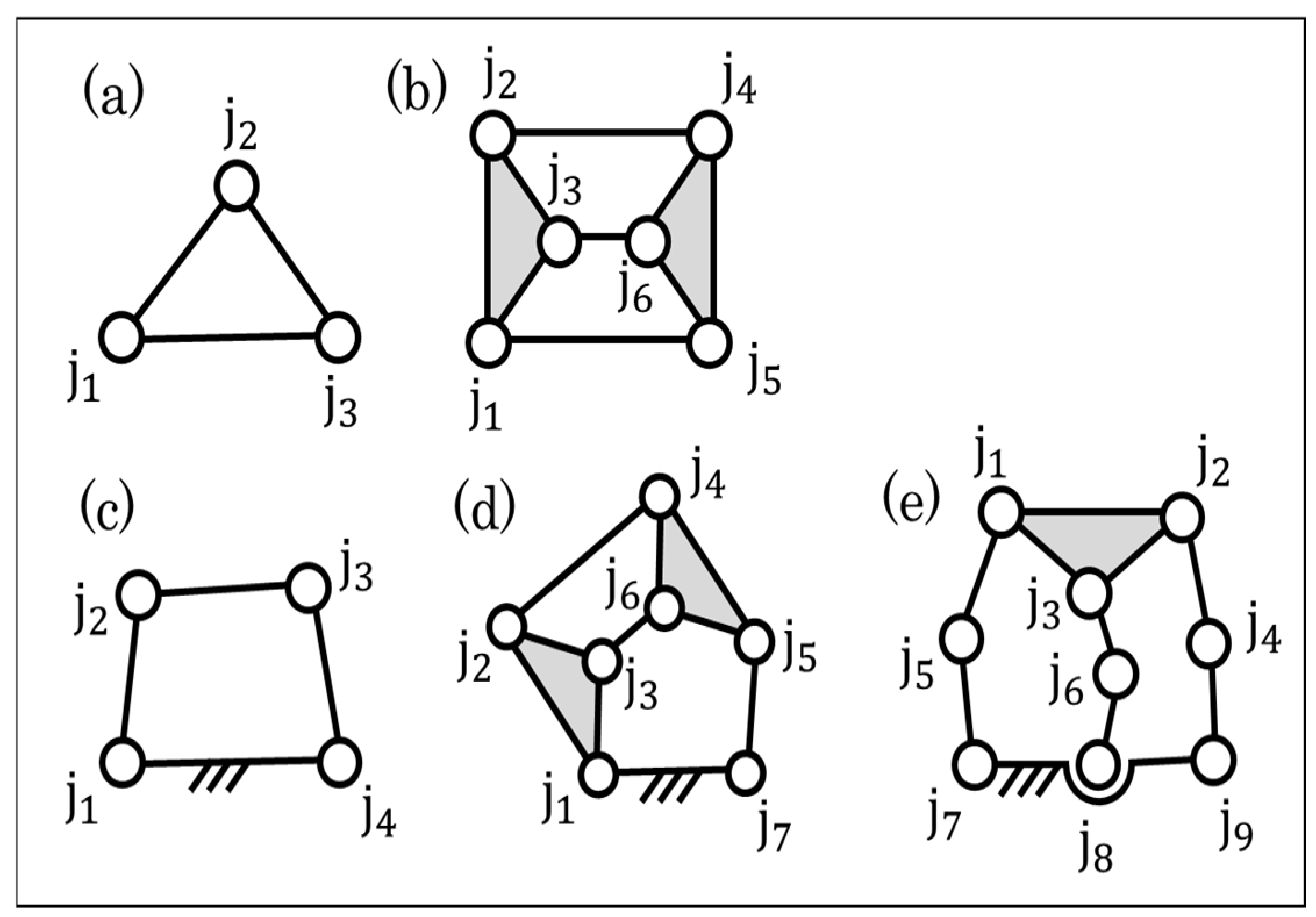
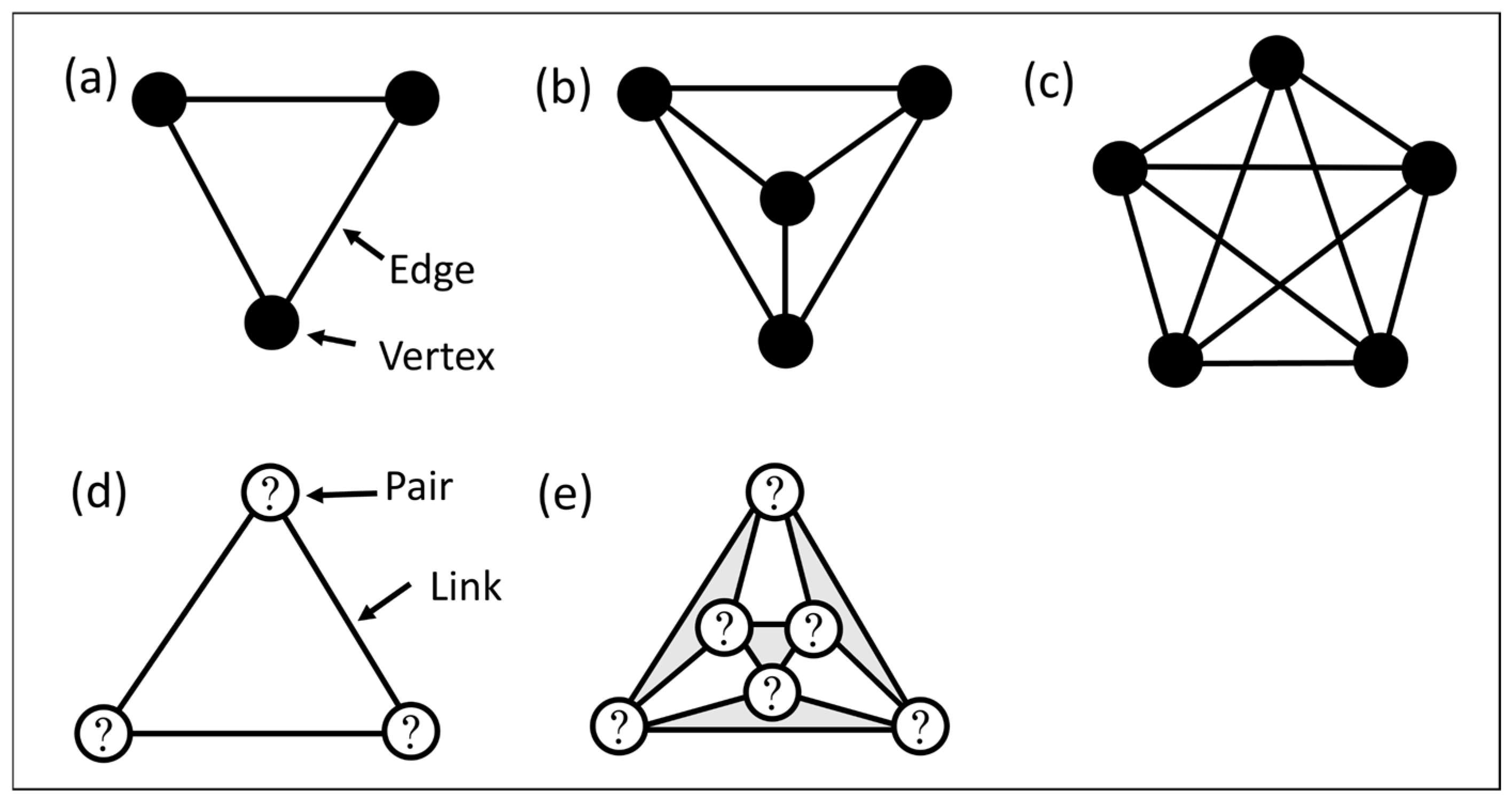
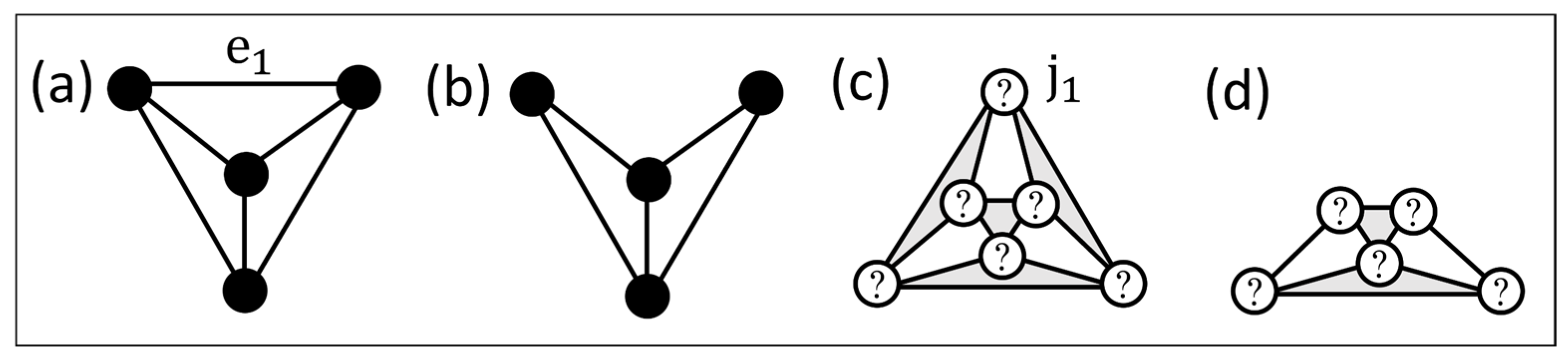
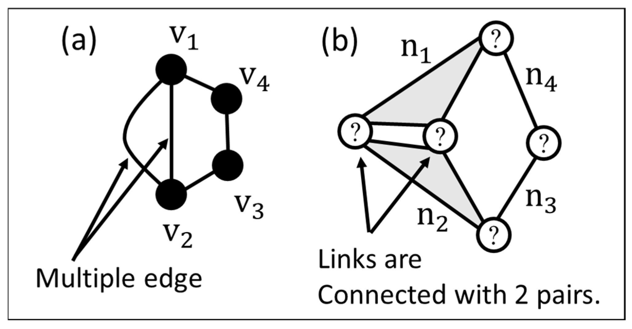
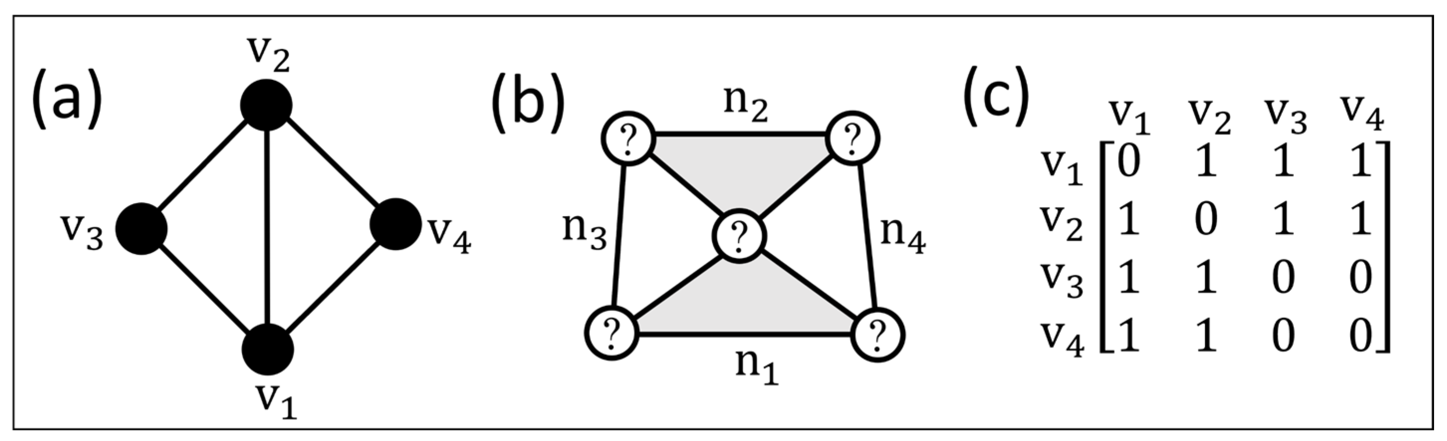
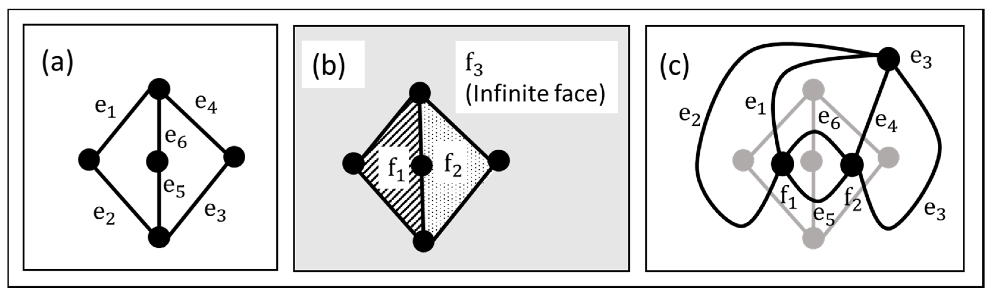
3.1. Graph Representation of Prime Structures
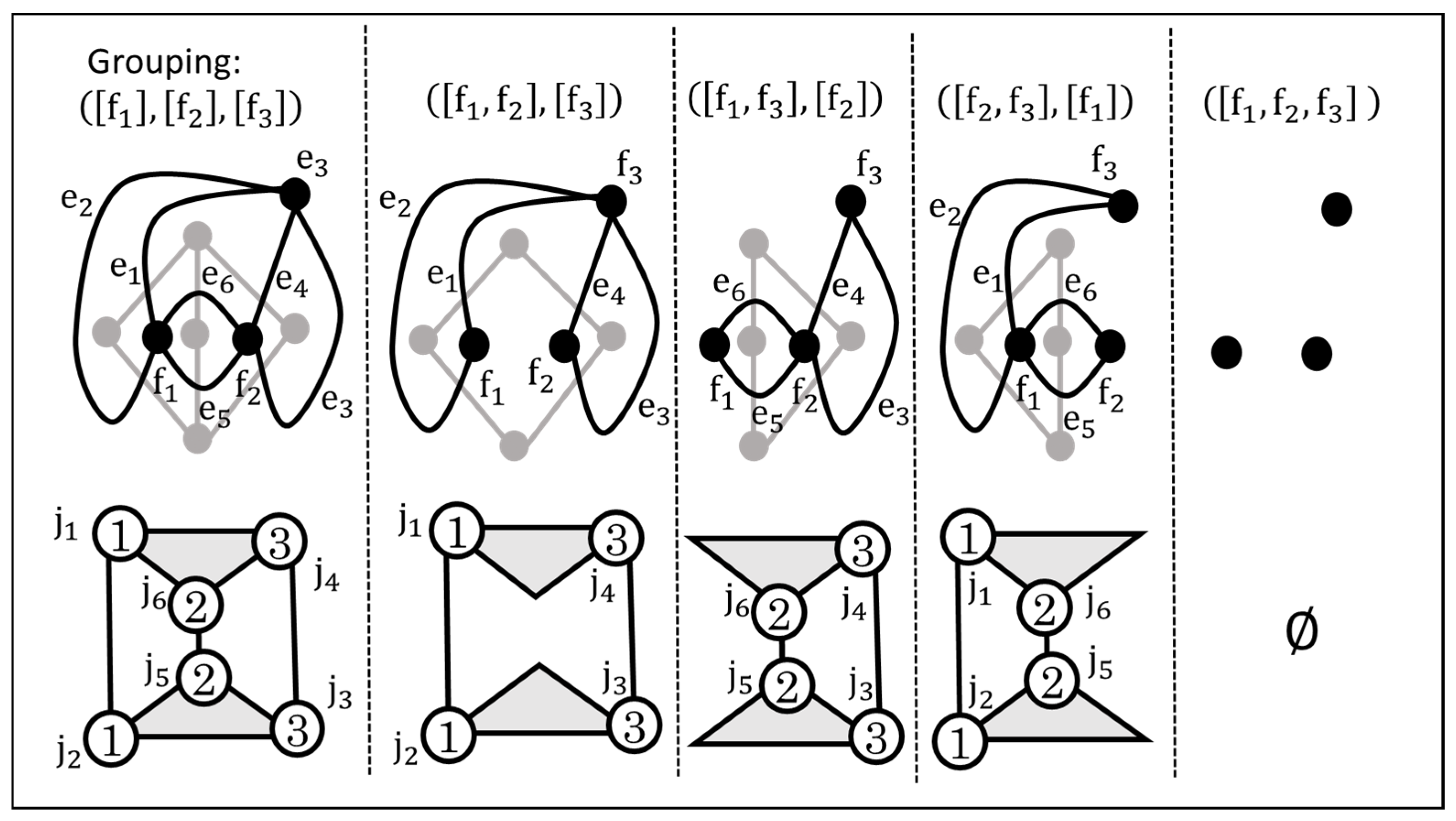
3.2. Exhaustive Enumeration of All Possible Link Connection Graphs
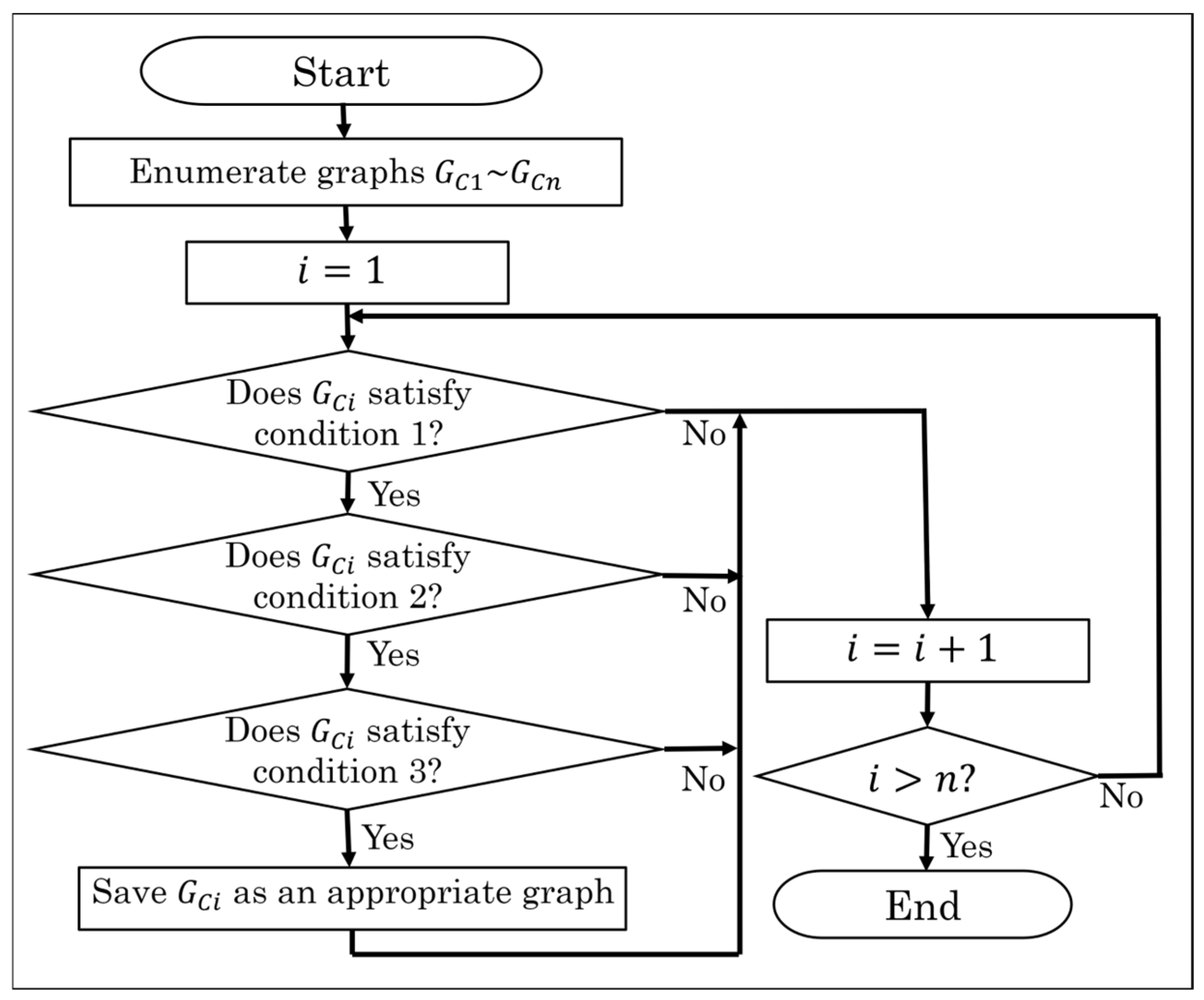
3.3. Elimination of the Inappropriate Link Connection Graphs
- Condition 1: The number of vertices with -degree is .
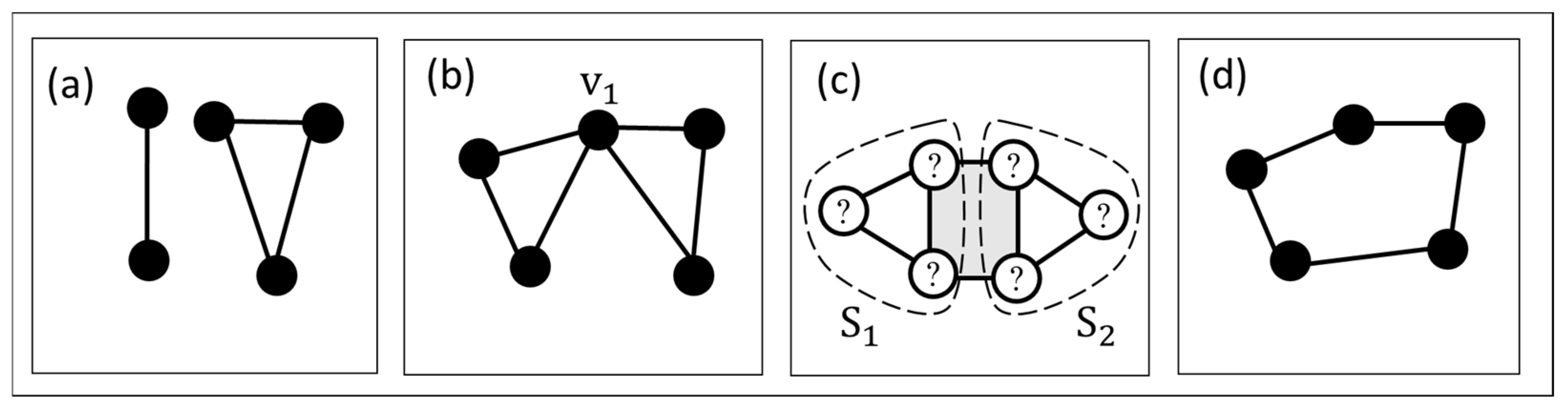
- Condition 2: The graph must be 2-connected.
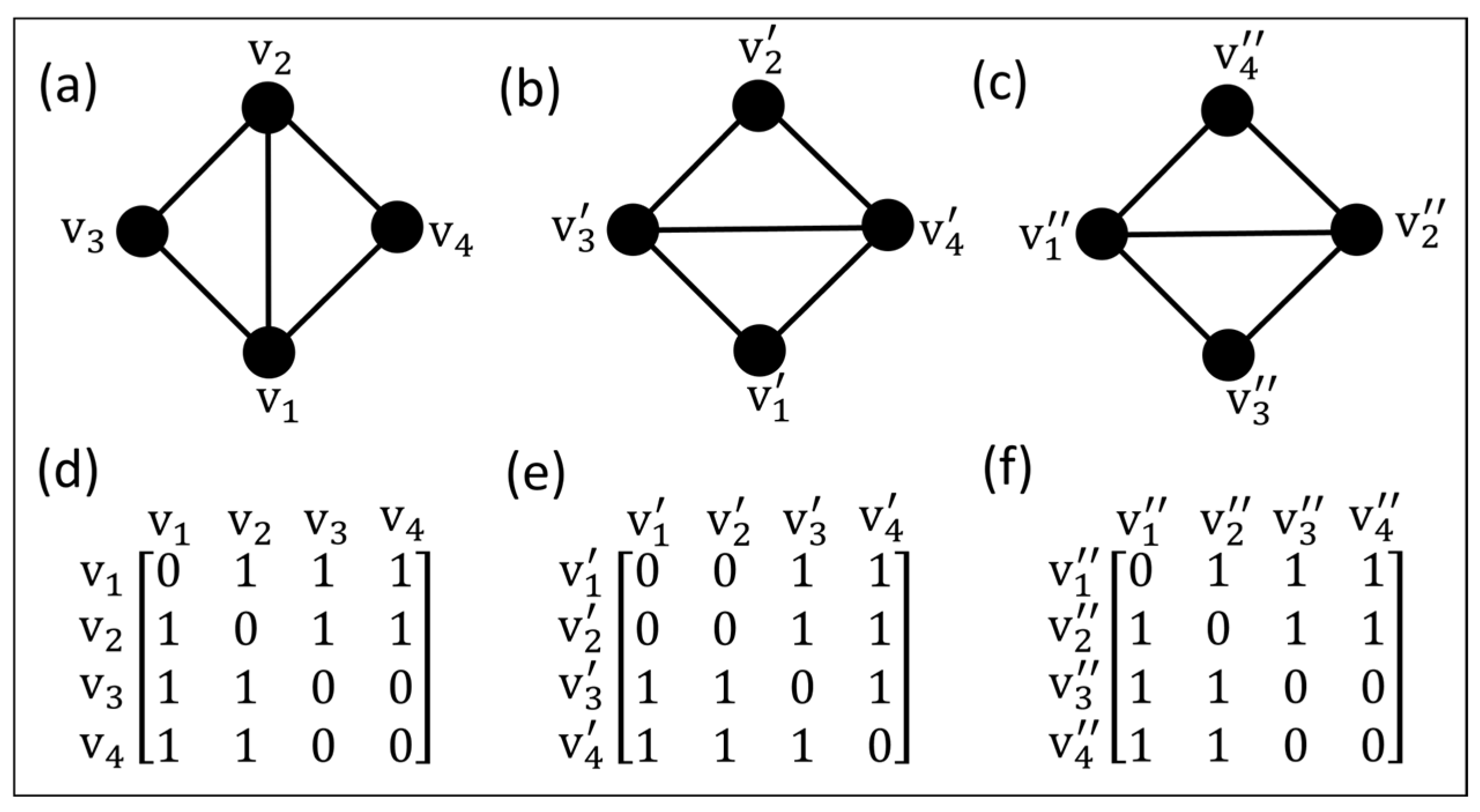
- Condition 3: There are no isomorphic graphs.
4. Pair Arrangement
4.1. Enumeration of the Pair Arrangement Graphs
4.2. Isomorphism Test
4.3. Primality Test
4.4. Consideration of Idle DoF
5. Results and Discussion
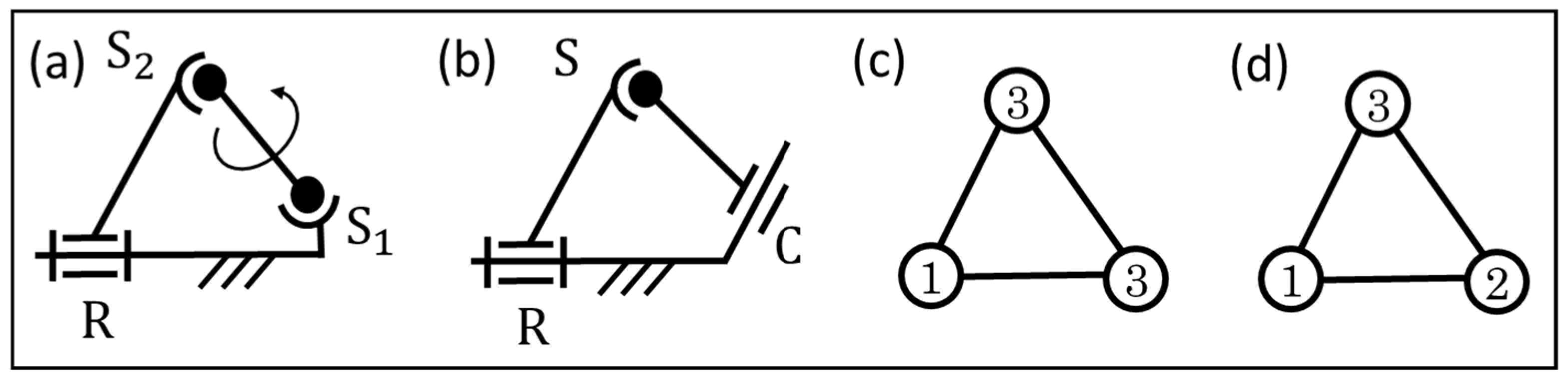
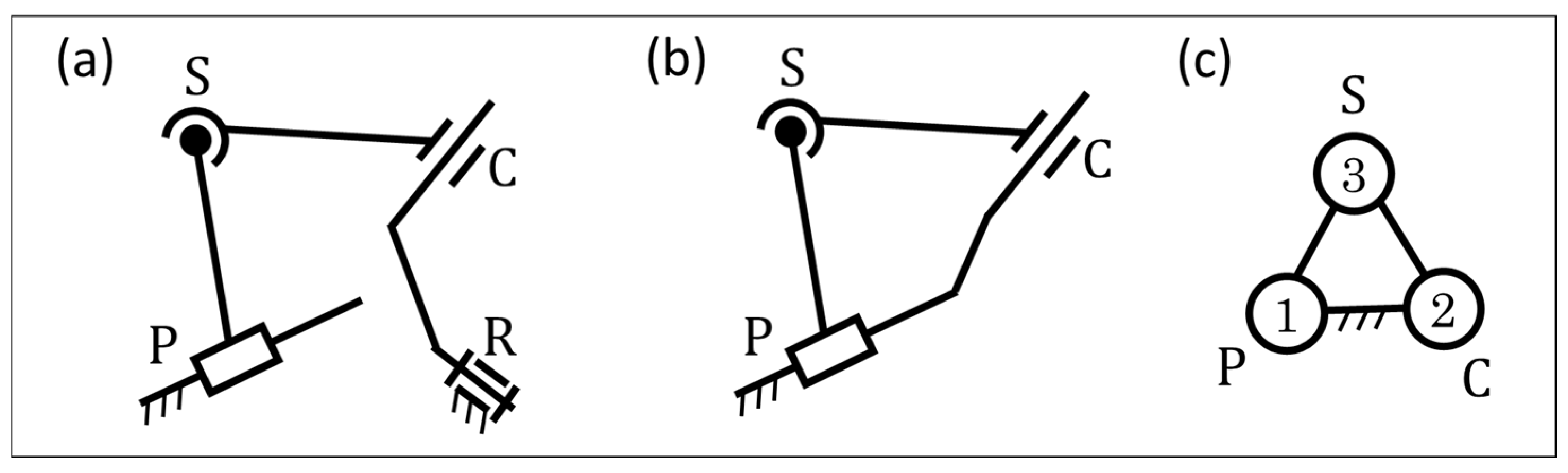
6. Kinematic Analysis of Spatial Mechanisms Using Spatial Prime Structures
7. Conclusions and Future Works
- (1)
- In order to consider the DoF of pairs, the enumeration method using two types of graphs—link connection graphs and pair arrangement graphs—are proposed.
- (2)
- The prime structures with idle DoF, which are given as rotation of a spherical–spherical binary link and do not exist in planar prime structure, are also enumerated.
- (3)
- As a result of the exhaustive enumeration, 3, 13, and 97 types of three-, four-, and five-link spatial prime structures are obtained, respectively.
- (4)
- Several examples of kinematics analysis based on configuration analyses of the enumerated spatial prime structures are shown.
Author Contributions
Funding
Data Availability Statement
Conflicts of Interest
References
- Funabashi, H. A Study on Completely Computer-Assisted Kinematic Analysis of Planar Link Mechanisms. Mech. Mach. Theory 1986, 21, 473–479. [Google Scholar] [CrossRef]
- Huang, P.; Ding, H. Structural Synthesis of Baranov Trusses with up to 13 Links. J. Mech. Des. 2019, 141, 072301. [Google Scholar] [CrossRef]
- Baranov, G. Classification, Formation, Kinematics, and Kinetostatics of Mechanisms with Pairs of the First Kind (in Russian). Proc. Semin. Theory Mach. Mech. 1952, 2, 15–39. [Google Scholar]
- Yan, H.S.; Hwang, W.M. Atlas of Basic Rigid Chains. In Proceedings of the 9th Applied Mechanisms Conference, Los Angeles, CA, USA, 18–23 August 1985; pp. 1.1–1.8. [Google Scholar]
- Yang, T.; Yao, F. Topological Characteristics and Automatic Generation of Structural Synthesis of Planar Mechanisms Based on the Ordered Single-Opened-Chains. In Proceedings of the 23rd Biennial Mechanisms Conference: Mechanism Synthesis and Analysis, Minneapolis, MN, USA, 11–14 September 1994; pp. 67–74. [Google Scholar]
- Galletti, C.U. A Note on Modular Approaches to Planar Linkage Kinematic Analysis. Mech. Mach. Theory 1986, 21, 385–391. [Google Scholar] [CrossRef]
- Liang, X.; Takeda, Y. Transmission Index of a Class of Parallel Manipulators with 3-RS (SR) Primary Structures Based on Pressure Angle and Equivalent Mechanism with 2-SS Chains Replacing RS Chain. Mech. Mach. Theory 2019, 139, 359–378. [Google Scholar] [CrossRef]
- Mruthyunjaya, T.S. Kinematic structure of mechanisms revisited. Mech. Mach. Theory 2003, 38, 279–320. [Google Scholar] [CrossRef]
- Yan, H.S.; Chiu, Y.T. On the number synthesis of kinematic chains. Mech. Mach. Theory 2015, 89, 128–144. [Google Scholar] [CrossRef]
- Rojas, N.; Thomas, F. On Closed-Form Solutions to the Position Analysis of Baranov Trusses. Mech. Mach. Theory 2012, 50, 179–196. [Google Scholar] [CrossRef]
- Chung, W.Y. Double Configurations of Five-Link Assur Kinematic Chain and Stationary Configurations of Stephenson Six-Bar. Mech. Mach. Theory 2007, 42, 1653–1662. [Google Scholar] [CrossRef]
- Pennock, G.R.; Kamthe, G.M. Study of dead-centre positions of single-degree-of-freedom planar linkages using Assur kinematic chains. Proc. Inst. Mech. Eng. Part C J. Mech. Eng. Sci. 2006, 220, 1057–1074. [Google Scholar] [CrossRef]
- Lee, C.C.; Lo, C.Y. Movable Focal-Type 7-Bar Baranov-Truss Linkages. In Proceedings of the ASME 2013 International Design Engineering Technical Conferences and Computers and Information in Engineering Conference, Portland, OR, USA, 4–7 August 2013; pp. 1–7. [Google Scholar]
- Kim, S.H.; Cho, C. Transformation of Static Balancer from Truss to Linkage. J. Mech. Sci. Technol. 2016, 30, 2093–2104. [Google Scholar] [CrossRef]
- Rojas, N.; Ma, R.R.; Dollar, A.M. The GR2 Gripper: An Underactuated Hand for Open-Loop In-Hand Planar Manipulation. IEEE Trans. Robot. 2016, 32, 763–770. [Google Scholar] [CrossRef]
- Nie, S.; Liao, A.; Qiu, A.; Gong, S. Addition Method with 2 Links and 3 Pairs of Type Synthesis to Planar Closed Kinematic Chains. Mech. Mach. Theory 2012, 58, 179–191. [Google Scholar] [CrossRef]
- Morlin, F.V.; Carboni, A.P.; Martins, D. Reconciling Enumeration Contradictions: Complete List of Baranov Chains with Up to 15 Links With Mathematical Proof. J. Mech. Des. 2021, 143, 083304. [Google Scholar] [CrossRef]
- Ding, H.; Huang, P.; Yang, W.; Kecskeméthy, A. Automatic generation of the complete set of planar kinematic chains with up to six independent loops and up to 19 links. Mech. Mach. Theory 2016, 96, 75–93. [Google Scholar] [CrossRef]
- Ding, H.; Huang, Z.; Mu, D. Computer-Aided Structure Decomposition Theory of Kinematic Chains and Its Applications. Mech. Mach. Theory 2008, 43, 1596–1609. [Google Scholar] [CrossRef]
- Ding, H.; Zhao, J.; Huang, Z. The Establishment of Edge-Based Loop Algebra Theory of Kinematic Chains and Its Applications. Eng. Comput. 2010, 26, 119–127. [Google Scholar] [CrossRef]
- Tuttle, E.R. Generation of Planar Kinematic Chains. Mech. Mach. Theory 1996, 31, 729–748. [Google Scholar] [CrossRef]
- Sunkari, R.P.; Schmidt, L.C. Structural synthesis of planar kinematic chains by adapting a Mckay-type algorithm. Mech. Mach. Theory 2006, 41, 1021–1030. [Google Scholar] [CrossRef]
- Simoni, R.; Carboni, A.P.; Martins, D. Enumeration of kinematic chains and mechanisms. Proc. Inst. Mech. Eng. Part C J. Mech. Eng. Sci. 2009, 223, 1017–1024. [Google Scholar] [CrossRef]
- Martins, D.; Carboni, A.P. Variety and Connectivity in Kinematic Chains. Mech. Mach. Theory 2008, 43, 1236–1252. [Google Scholar] [CrossRef]
- Ding, H.; Zhao, J.; Huang, Z. Unified Structural Synthesis of Planar Simple and Multiple Joint Kinematic Chains. Mech. Mach. Theory 2010, 45, 555–568. [Google Scholar] [CrossRef]
- Jinkui, C.; Weiqing, C. Systemics of Assur Groups with Multiple Joints. Mech. Mach. Theory 1998, 33, 1127–1133. [Google Scholar] [CrossRef]
- Funabashi, H.; Ogawa, K.; Hara, T. A Displacement Analysis of Spatial Four-Bar Mechanisms. Bull. JSME 1978, 21, 1521–1527. [Google Scholar] [CrossRef]
- Takeda, Y.; Funabashi, H.; Ichimaru, H. Development of Spatial In-Parallel Actuated Manipulators with Six Degrees of Freedom with High Motion Transmissibility. JSME Int. J. Ser. C 1997, 40, 299–308. [Google Scholar] [CrossRef]
- Cronin, D.L. MacPherson strut kinematics. Mech. Mach. Theory 1981, 16, 631–644. [Google Scholar] [CrossRef]
- Iwatsuki, N. Kinematic Analysis and Design of Suspension-steering Mechanisms for Vehicles. JTEKT Eng. J. 2023, 1019E, 3–13. [Google Scholar]
- Gosselin, C.; Angeles, J. Singularity analysis of closed-loop kinematic chains. IEEE Trans. Robot. Autom. 1990, 6, 281–290. [Google Scholar] [CrossRef]
- Wu, T.L.; Chen, J.H.; Chang, S.H. A six-DOF prismatic-spherical-spherical parallel compliant nanopositioner. IEEE Trans. Ultrason. Ferroelectr. Freq. Control 2008, 55, 2544–2551. [Google Scholar]
- Yu, Y.Q.; Feng, Z.L.; Xu, Q.P. A pseudo-rigid-body 2R model of flexural beam in compliant mechanisms. Mech. Mach. Theory 2012, 55, 18–33. [Google Scholar] [CrossRef]


| (1) Number of links | 3 | 4 | ||||||
| (2) Numbers of 1, 2, 3-DoF pairs | ||||||||
| (3) Numbers of links with 2, 3 pairs | ||||||||
| (4) Link connection topology |  | N/A |  |  |  | |||
| (5) Prime structures |  |  |  |  |  |  |  | |
| (6) Prime structures with idle DoFs |  |  |  | |||||
| (1) Number of links | 5 | ||
| (2) Numbers of 1, 2, 3-DoF pairs | |||
| (3) Numbers of links with 2, 3, 4 pairs | |||
| (4) Link connection topology |  |  |  |
| (5) Prime structures | 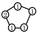 | DOFs of | |
| (6) Prime structures with idle DoFs | DOFs of | ||
| (1) Number of links N | 5 | |||
| (2) Numbers of 1, 2, 3-DoF pairs | ||||
| (3) Numbers of links with 2, 3, 4 pairs | ||||
| (4) Link connection topology | 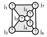 |  | 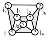 | 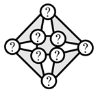 |
| (5) Prime structures |  | |||
| (6) Prime structures with idle DoFs | ||||
Disclaimer/Publisher’s Note: The statements, opinions and data contained in all publications are solely those of the individual author(s) and contributor(s) and not of MDPI and/or the editor(s). MDPI and/or the editor(s) disclaim responsibility for any injury to people or property resulting from any ideas, methods, instructions or products referred to in the content. |
© 2024 by the authors. Licensee MDPI, Basel, Switzerland. This article is an open access article distributed under the terms and conditions of the Creative Commons Attribution (CC BY) license (https://creativecommons.org/licenses/by/4.0/).
Share and Cite
Aruga, T.; Iwatsuki, N. Exhaustive Enumeration of Spatial Prime Structures. Machines 2024, 12, 529. https://doi.org/10.3390/machines12080529
Aruga T, Iwatsuki N. Exhaustive Enumeration of Spatial Prime Structures. Machines. 2024; 12(8):529. https://doi.org/10.3390/machines12080529
Chicago/Turabian StyleAruga, Takahiro, and Nobuyuki Iwatsuki. 2024. "Exhaustive Enumeration of Spatial Prime Structures" Machines 12, no. 8: 529. https://doi.org/10.3390/machines12080529
APA StyleAruga, T., & Iwatsuki, N. (2024). Exhaustive Enumeration of Spatial Prime Structures. Machines, 12(8), 529. https://doi.org/10.3390/machines12080529