Article

A Terminal Residual Vibration Suppression Method of a Robot Based on Joint Trajectory Optimization

1
College of Information Science and Engineering, Northeastern University, Shenyang 110819, China
2
SIASUN Robot & Automation Co., Ltd., Shenyang 110168, China
3
Faculty of Robot Science and Engineering, Northeastern University, Shenyang 110169, China
*
Author to whom correspondence should be addressed.
Machines 2024, 12(8), 537; https://doi.org/10.3390/machines12080537
Submission received: 6 July 2024 / Revised: 29 July 2024 / Accepted: 2 August 2024 / Published: 6 August 2024

Abstract

:
Vibration problems have become one of the most important factors affecting robot performance. To this end, a terminal residual vibration suppression method based on joint trajectory optimization is proposed to improve the accuracy and stability of robot motion. Firstly, based on the characteristics of the friction nonlinearity due to joint coupling and physical feasibility of dynamic parameters, a semidefinite programming method is used to identify dynamic parameters with actual physical meaning, thereby obtaining an accurate dynamic model. Then, based on the result of the residual vibration time domain analysis, a joint trajectory optimization model with the goal of minimizing joint tracking error is established. The Chebyshev collocation method is used to discretize the optimization model. The dynamic model is used as the optimization constraint, and barycentric interpolation is used to obtain the optimized joint motion trajectory. Finally, industrial robot experiments prove that the vibration suppression method proposed in this article can reduce the maximum acceleration amplitude of residual vibration by 62% and the vibration duration by 71%. Compared with the input shaping method, the method proposed in this paper can reduce the terminal residual vibration more effectively and ensure the consistency of running time and trajectory.

1. Introduction

With the development of science and technology and the rise in industrial automation, industrial robots perform tasks through efficient and precise movements, improving productivity, reducing costs, and creating a safer working environment for humans [1,2,3]. The flexible characteristics of industrial robot joint transmission parts like the RV reducers and gears reduce the overall stiffness of the robot, making it have a more complex vibration mode and easier to vibrate during and after the movement [4,5]. Such vibration problems have become one of the most important factors affecting the performance and stability of robots. Robot vibration suppression technology reduces or eliminates robot vibration through advanced control strategies and design methods, thereby improving motion accuracy and stability.
With an accurate system model, motion profiles or feedforward control can be generated based on optimal trajectory planning to minimize overshoot and residual vibration. Based on the chaotic particle swarm optimization algorithm, the trajectory interpolation parameters can be optimized with the minimum vibrational deformation of the flexible end as the objective function [6]. In reference [7], the dynamic equation of the flexible curve connecting rod was derived by using the absolute nodal coordinate formula, and the optimal trajectory method was used to generate the trajectory with the least vibration of the flexible curve connecting rod. In reference [8], the trajectory planning problem of suppressing the residual vibration of the robot was transformed into the optimal control performance problem, and the Fourier series was used to fit the discrete optimal trajectory. The authors of [9] proposed a torque feedforward damping strategy based on the chaotic regression tree dynamics model to improve the motion accuracy of the robot in the process of low-speed motion and suppress the vibration of the robot. In reference [10], coprime factorization-based feedforward control and H∞ control are cooperatively applied to the quasi-full-closed-loop control structure, forming a fundamental control strategy with improved reference tracking and residual vibration suppression capability. Reference [11] adopted a fully compensated feedforward torque control method based on the dynamic model, and compared with other feedforward methods, the robot has the fastest response speed and the lowest joint trajectory tracking error and jitter. However, the above methods have high requirements for the model and parameter accuracy of the system, otherwise the interference caused by the uncertain disturbance inside the robot will affect the algorithm control effect.
If an accurate model is not available but the states associated with elastic vibrations can be measured or observed, singular perturbations [12,13] and nonlinear feedback control [14,15] can be implemented to accommodate unmodeled dynamics and perturbations. Reference [16] proposed a novel high-performance multilayer neurocontroller which can simultaneously reject matched and mismatched disturbances like vibrations. Iterative learning control is another option to solve these problems, and optimal feedforward control can be implemented through learning when robots perform the same tasks repeatedly [17]. Compared with the above methods, the input shaping method can effectively minimize overshoot and residual vibration, and it does not require complex dynamic models, there is no need for the direct measurement of elastic vibrations for online feedback, and no need for repetitive tasks. However, one disadvantage of the use of input shaping in industrial robots is the time delay, which can slow down the overall task for applications with fast stationary to stationary motion such as spot welding, handling, etc. References [18,19] proposed an improved zero-delay input shaping so that no delay was introduced. However, this kind of shaping algorithm depends on the vibration frequency parameter of the robot body, and the frequency change in different postures of the robot will affect the shaping effect. In addition, input shaping may change the original motion trajectory, and for applications with high trajectory accuracy requirements such as arc welding and gluing, changing the motion trajectory will reduce the quality of the work.
In order to solve the above problems, this paper proposes a terminal residual vibration suppression method based on joint trajectory optimization. Firstly, a piecewise nonlinear friction model is designed according to the coupling characteristics of the robot joints, and the semi-definite programming is used to identify the dynamic parameters and friction parameters with physical significance synchronously, so as to obtain the accurate dynamic characteristics of the robot. Then, a method to transform Cartesian space trajectory vibration suppression into joint space trajectory optimization is proposed, and the optimization of the initial state and objective function is designed, which can ensure the consistency of trajectory optimization on the basis of terminal vibration suppression.

2. Identification of Dynamic Parameters Based on Physical Feasibility Constraints

Due to the complexity of the robot components and assembly errors, it is difficult to know the robot dynamics accurately. However, it was found that the dynamic characteristics of the robot are a linear function of its inertial parameters [20], so the problem of obtaining the inertial parameters of the robot can be transformed into a system of linear equations. First, the robot dynamics equation is rewritten into a linear parametric form, as shown in (1)
τ = Y q , q ˙ , q ¨ β
where τ is the vector of joint torque, β N b is the reorganization parameter vector which is called minimum inertia parameter, and Y q , q ˙ , q ¨ n × N b is the full-rank observation matrix obtained after reorganization. Afterwards, by controlling robot by joint excitation trajectory and collecting the torque value of each joint in the process to obtain a group of test data, Formula (2) is obtained according to (1)
Γ = W β + ρ
where W = Y ( q ( t 1 ) , q ˙ ( t 1 ) , q ¨ ( t 1 ) ) n × N b , , Y ( q ( t M ) , q ˙ ( t M ) , q ¨ ( t M ) ) n × N b T is the observation matrix, ρ is the observation error due to various reasons, and Γ = [ τ ( t 1 ) T τ ( t 2 ) T τ ( t M ) T ] T is the joint torque value corresponding to the test data. Finally, according to the least squares method, the minimum inertia parameter estimation vector β ^ can be obtained.
Constructing an accurate friction model is an important part of improving the accuracy of the dynamic model, and it is difficult for a single friction model to fully fit the diverse joint features. For coupling joints of an industrial robot, the friction between two joints interacting with each other produces characteristics that differ from the standard friction model. Therefore, the friction model f j of the coupling joint j is designed as Equation (3)
f j = F c j 1 sign ( q ˙ j ) + F v j 1 q ˙ j , q ˙ s q ˙ j < q ˙ l F c j 2 sign ( q ˙ j ) + F v j 2 q ˙ j , q ˙ j q ˙ l
where q ˙ s and q ˙ l are pre-identified parameters for the friction model. F c j m and F v j n are the parameters to be identified with minimum inertial parameters synchronously.
The minimum inertial parameters calculated by the least squares method can only identify linear combinations of parameters and cannot assert the physical feasibility directly. Therefore, it is necessary to add feasibility constraints to the calculation of dynamic parameter identification to obtain the standard parameter form that satisfies the definition of physics. For the connecting rod k, the parameter δ k to be identified is defined as
δ k = L k , x x , L k , x y , L k , x z , L k , y y , L k , y z , L k , z z , l k , x , l k , y , l k , z , m k
For a six-joint industrial robot, the mass of connecting rod k must be positive, and the inertial tensor is symmetrical and positive definite. The set of available physical feasibility constraints for the robot is expressed as
Ω = δ n : m k > 0 , L k 1 m k S l k T S l k 0   |   k = 1 , , 6
where L k is the inertial tensor of the connecting rod k with respect to the coordinate system of the connecting rod, l k is the first moment of the vector of inertia, and S is a partial symmetric matrix operator. Combined with the parameters of the friction model f p , i of each joint, the linear matrix inequality of the physical feasibility dynamic parameters is obtained as
D δ = d i a g D δ 1 , , D δ 6 , f p , 1 , , f p , 6 0
Since there is a one-to-one mapping relationship G between the minimum inertia parameters β , the independent terms δ d δ in the parameters to be identified, and the linkage dynamics parameters [21], the physical feasibility constraints can be transformed into the constraints of the minimum inertia parameters and independent parameters, as shown in (7)
D β β , δ d = D δ = D G 1 β , δ d
u is defined as the distance of the actual and identified values of the minimum inertial parameters as shown in (8)
u = Γ W β 2 = Γ W β T Γ W β
Convert (8) into a linear matrix inequality form as (9)
U ω u , β = u Γ W β T Γ W β 1 0
In summary, the problem of solving the dynamic parameters based on the constraints of physical feasibility can be expressed as the following form of SDP:
min ( u , β , δ d ) u
s . t . F u , β , δ d 0
where the linear matrix inequality constraints are defined as (12)
F u , β , δ d = U ω u , β 0 0 D β u , β
For the optimization problem described in (10), (11), and (12), the optimal solution u * is the sum of the identification errors under constraints, and the standard parameters δ * of robot dynamics satisfying the physical feasibility constraints can be calculated from the mapping of the δ d * and β * .

3. Residual Vibration Suppression Based on the Optimal Trajectory Principle

Unlike the conventional position motion of the robot, the residual vibration is characterized by a small oscillation with the position at the end of the trajectory as the equilibrium point. Bringing the joint vibration response into the forward kinematics model of the robot, it can be seen that the wrist position of the robot during residual vibration is [8]
p x e = p = 1 N E p cos ω p t ϕ p p y e = p = 1 N F p cos ω p t ϕ p p z e = p = 1 N G p cos ω p t ϕ p
where E p , F p , and G p are the amplitude of item p. The position error of the robot P e ( t ) in cartesian space is a function of the joint position error and velocity error at the end time. Therefore, the problem of reducing residual vibration can be transformed into a problem of reducing the position and velocity error at the end time.
On the basis of the initial value of the trajectory, the optimal trajectory problem can be obtained by setting up objective functions and constraints to meet the requirements [22]. The optimal trajectory algorithm designed in this paper includes three steps: initial trajectory discretization, establishment and solution of objective function and constraints, and barycentric interpolation.

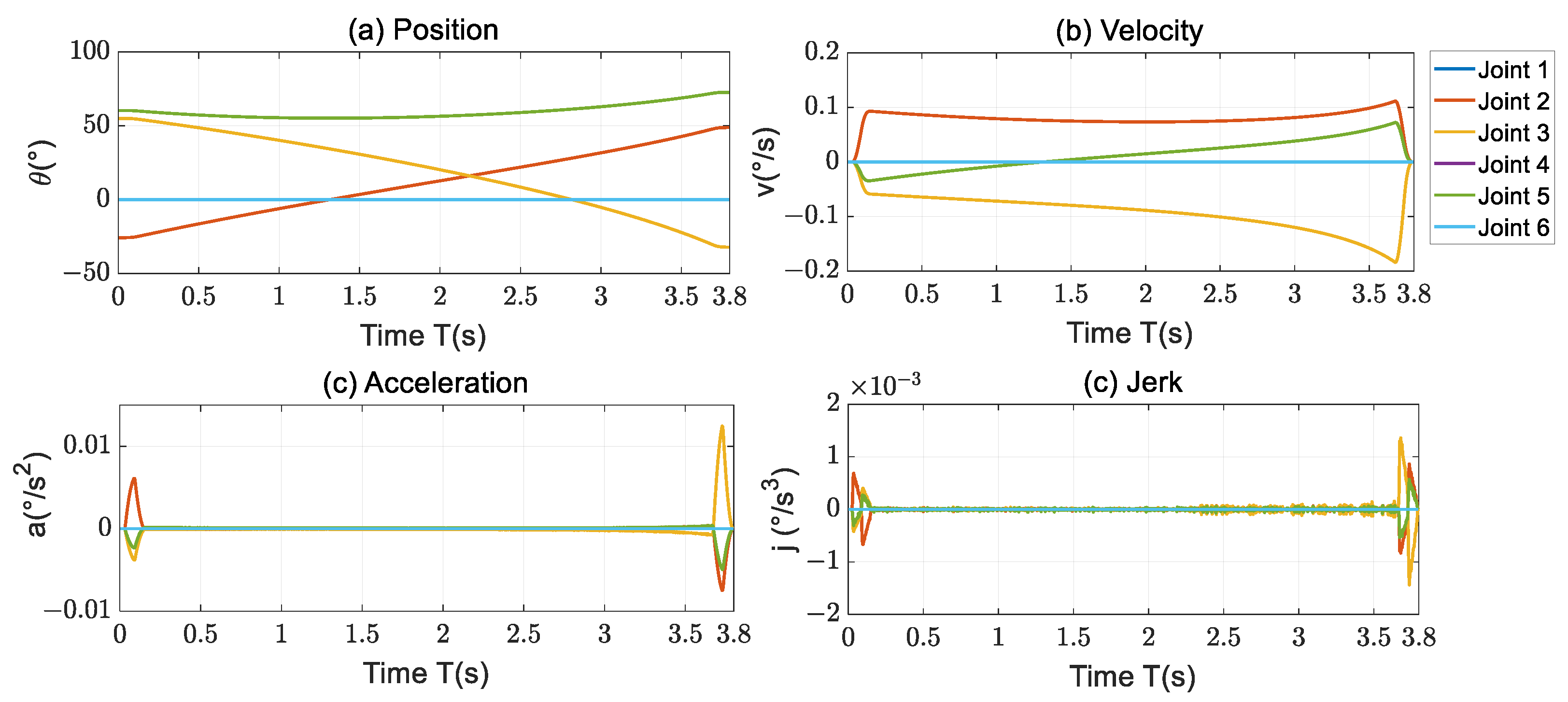
3.1. Initial Trajectory Discretization

According to the robot kinematic model, due to the nonlinear mapping of the terminal pose and the joint angle, the acceleration discontinuity or abrupt change will still occur in the joint space, so the optimization calculation will be carried out in the joint space. For cartesian space trajectory P ( t ) , 0 t t f , the angle of each joint in each control cycle is q p , i t , on which Chebyshev collocation [22] is performed as shown in (14)
q p , i T k = q p , i t f cos k π / N + 1 / 2 , k = 0 , , N
where q p , i T 0 and q p , i T N are the joint values corresponding to the initial and ending positions of the trajectory respectively.
One of the advantages of using the polynomial coordination method is that the differential matrix D can be used to derive the variables on the nodes quickly and accurately, so the differential of the position and torque of each joint are shown in (15)
d q p , i T k / d T = 2 D q p , i T k / t f d τ p , i T k / d T = 2 D τ p , i T k / t f

3.2. Objective Functions and Constraints

Define the position and velocity of each joint as the optimal problem state variables, and the joint torque as the control variable, as shown in (16)
x T k = q T k , q ˙ T k T u T k = τ T k
Under the premise that the tracking performance of the control system is guaranteed, the problem of minimizing the position and speed error of the whole process and the start and stop points can be further simplified to the minimum acceleration change rate during motion, so the discretized optimization objective function is obtained as follows
J = k = 1 N u ˙ ( T k ) T W R u ˙ ( T k )
where W R is the weighted diagonal matrix. Theoretically, the greater the inertia, the greater the joint weight is.
The dynamic parameters identified by (10)–(12) can establish more accurate dynamic constraints for each joint, as shown in (18)
u T k = DYN x T k , δ *
In addition, the position and velocity of the start and end moments of each joint are used as equation constraints, and the position limit, velocity limit, and acceleration limit of each joint are used as inequality constraints at nodes to ensure that the robot starts and stops running. After the above discretization and design of the optimization objective function, the problem of the minimum error of position and velocity at the end point has been transformed into a typical nonlinear programming (NLP) problem with constraints. The algorithm based on the gradient descent principle can be used to solve the optimal control quantity u * T k and state quantity x * T k at the node.

3.3. Barycentric Interpolation

Since the calculated optimal state quantity is the value at each node after discretization, it is necessary to select an interpolation algorithm to convert it into the joint position value of each control cycle. The node-based polynomial fitting is achieved by barycentric interpolation [23], which can be expressed as a linear combination of Lagrange polynomials, and the optimized angles of each joint are obtained as shown in (19)
q ^ t = j = 0 N q * T j l j t
where l j t is the j-th Lagrange polynomial, defined as (20)
l j t = k = 0 N t T k v j t T j
where v j is the imputation weight corresponding to node j. For node-based polynomial interpolation, the error of the optimized trajectory and the original trajectory at the node is 0, and the error between the nodes can be obtained by (21)
ε t = P ( t ) KINE q ^ ( t )
Based on the above calculations, the motion trajectory with the same number of interpolation points as the pre-optimization trajectory is obtained again, which not only ensures that the optimized start–stop position is the same as the original trajectory but also ensures the consistency between the optimized running trajectory and the original trajectory. The joints of the robot are controlled to complete the movement according to the optimized trajectory, so as to reduce the amplitude and duration of residual vibration.

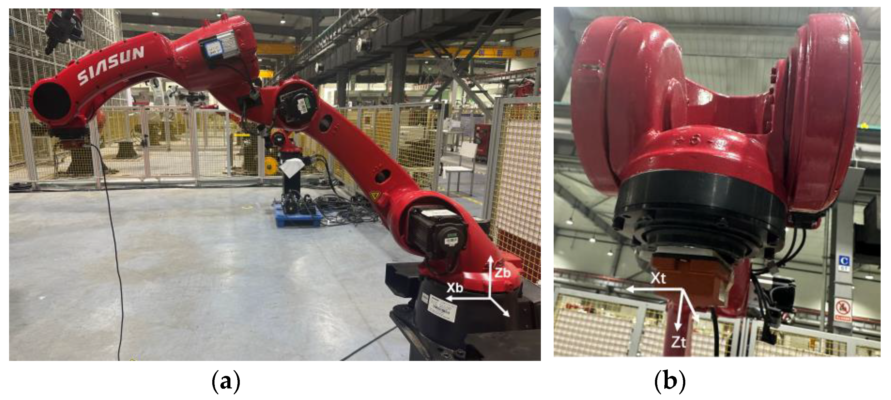
4. Experimental Verification and Analysis of Results

The industrial robot T12B is selected for experimental analysis, and the inertial sensor is selected for vibration testing. The parameters are shown in Table 1. The experiment is divided into two steps, the dynamic parameters are identified first, and then the residual vibration suppression experiment is carried out based on the identification results.

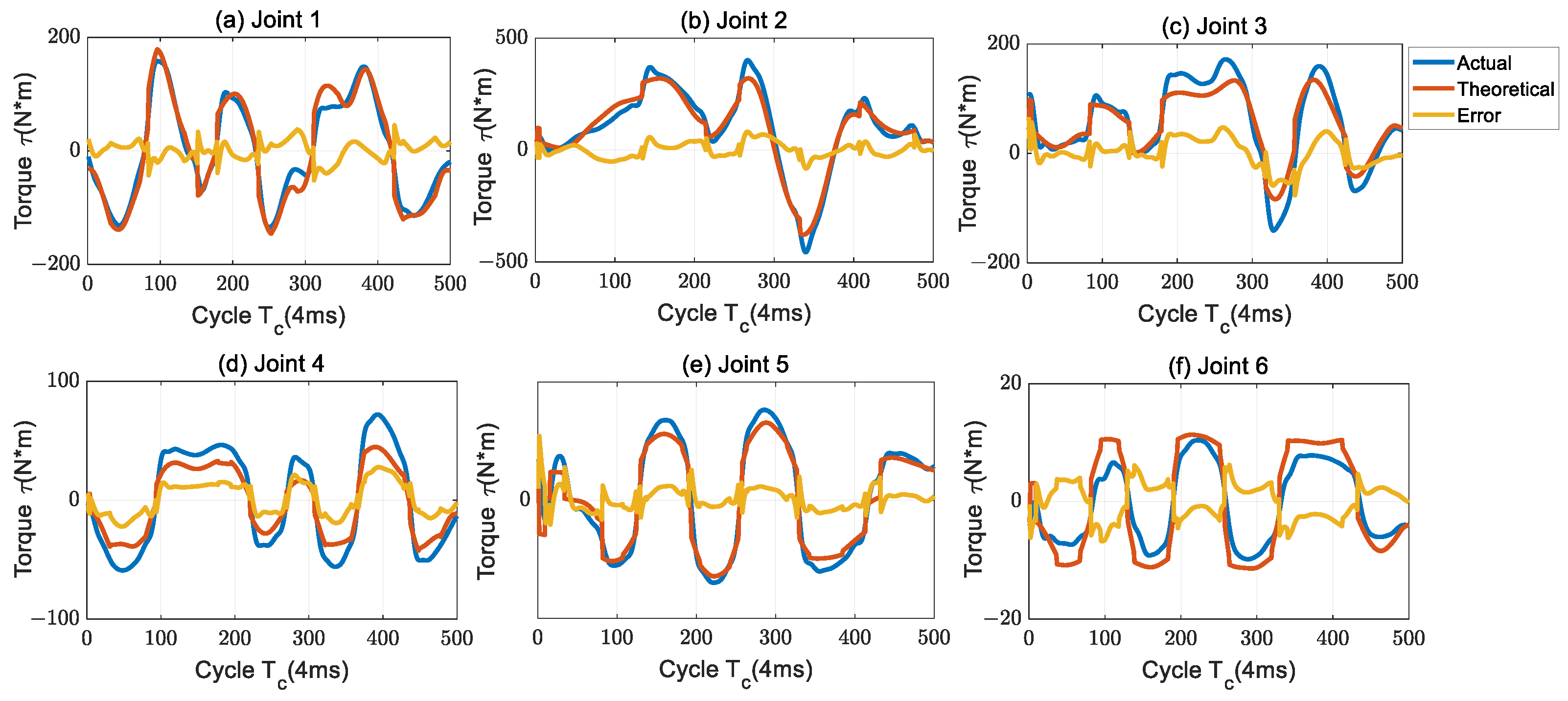
4.1. Identification of Dynamic Parameters

The excitation trajectory based on the Fourier series function [24] is selected to control the robot motion, the joint position and torque information are collected, and the dynamic parameters are calculated according to the identification algorithm. Then, the verification trajectory different from the excitation trajectory is selected, the actual torque of each joint during the movement is recorded, and the theoretical torque value is calculated according to the identification parameters and the difference between the two torques is compared to verify the correctness and accuracy of the identification results.
The minimum inertial parameters without considering the constraints of physical feasibility are used, and the dynamic parameter identification results are calculated by the least squares method. The actual torque of each joint and the theoretical torque based on the identified parameters are plotted as shown in Figure 1. It can be seen from the figure that the theoretical torque and the actual torque have a large spike protrusion when the velocity direction changes, and there is always a certain range of error in the constant velocity section.
According to the coupling characteristics of the T12B robot and the unified identification method of joint friction, the friction model such as Equation (3) is selected, and the friction model is included in the identification parameter set. The same excitation trajectory is selected, and the test data are substituted into Equations (10)–(12) to calculate the kinetic parameters that meet the constraints of physical feasibility. The recalculated kinetic parameters are shown in Table 2, and the identified friction parameters are shown in Table 3.
The parameters of Table 2 are brought into the dynamic formula, and the friction of the joint is calculated according to the friction parameters in Table 3. The actual output torque of each joint and the theoretical torque based on the identified parameters are plotted as shown in Figure 2. Compared with Figure 1, it can be seen that the peak protrusion of the theoretical and actual torque is significantly reduced when the velocity direction changes, and the accuracy in the uniform velocity section is significantly improved, especially the torque errors of joints 3, 4, and 6 are improved significantly.
The root mean square error (RMS) of the theoretical torque and the actual torque of the identification model are shown in Table 4. According to the RMS results, the theoretical value of the torque in the whole process is closer to the actual torque value identified by the constraint-based inertia parameters. Compared with the identification results of the unconstrained and frictionless model, the results of the 4, 5, and 6 joints proposed in this paper are improved by about 80% compared with the original algorithm, which shows that the algorithm has a significant effect on coupling joints and friction-sensitive joints.

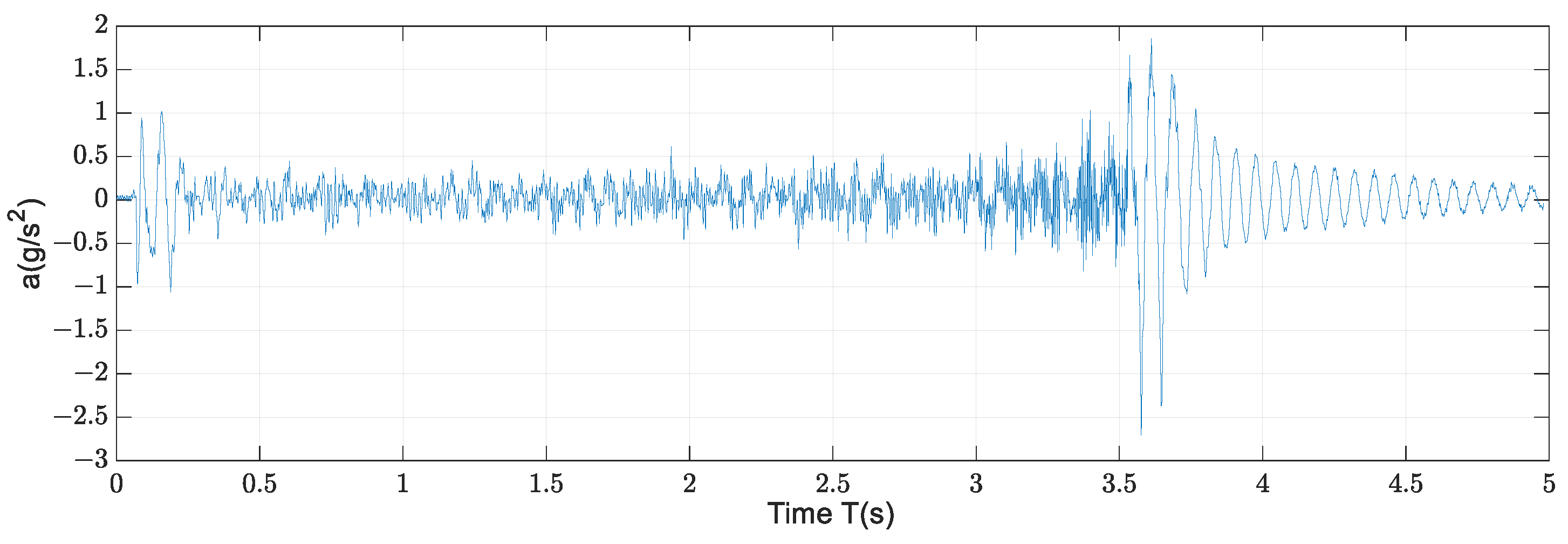
4.2. Verification of the Performance of Vibration Suppression

As shown in Figure 3, the robot moves in a straight line from position P1 to position P2 with a linear speed of 200 mm/s. P1 and P2 are (590, 0, 294) and (1317, 0, 294), respectively, under the base coordinate, and the unit is mm. An inertial sensor is installed at the flange to measure vibration during motion.
The experimental trajectory is the linear motion in cartesian space with no displacement in the Y-axis and Z-axis directions. The velocity in the X-axis direction is an S-shaped curve, which ensures a smooth velocity in cartesian space. From the kinematic model, it can be seen that the X-axis direction movement is mainly generated by the linkage of joints 2, 3, and 5, as shown in Figure 4.
However, due to the nonlinearity of the kinematic inverse solution, the above-mentioned joints produce a large velocity step at the start–stop point. In particular, in the deceleration stage of joint 3 at the stop point, the joint acceleration produces a peak value of 0.012, which is about 4 times the peak acceleration value of the initial stage. The sudden change in acceleration of the deceleration section leads to a large tracking error, which causes residual vibration at the end of the robot.
The acceleration curve in the Z direction of the terminal is obtained by the inertial sensor, as shown in Figure 5. As can be seen from the figure, the vibration with an amplitude of less than 1 in the Z direction at the beginning of the motion quickly converges to less than 0.5 with the motion. In the stop deceleration phase, the end amplitude is about three times that of the starting segment due to the abrupt change in acceleration, and a significant damping oscillation is generated.
According to the optimization model established in this paper, the kinetic parameters identified in Table 1 are brought into the dynamic constraints, the number of collocation nodes is selected as N = 12, the threshold of the number of iterations is 10, the solution time is 0.2 s, and the motion curve of the optimized joint is obtained as shown in Figure 6.
After optimization, the start and stop points of the position curve of each joint are the same as those of the original curve, and the running time is the same. From Equation (21), it can be seen that there is a maximum error of 0.5 mm between the trajectory and the original trajectory during the process, which ensures the consistency of the running trajectory. The acceleration amplitude of joint 2 and joint 3 in the stop phase is about 0.5 times that of the original trajectory, and the jerk amplitude is basically the same as that of the original trajectory.
After optimization, the vibration at the end of the robot during operation was re-measured, there was no visible vibration at the end of the entire operation stage, and the vibration curve of the stop section is shown in Figure 7. At the same time, the joint input shaping method is used to obtain the movement trajectory, the input shaping frequency is 8 Hz, the damping ratio is 0.4, and the delay of about 0.4 s is generated compared with the original trajectory, as shown in Figure 7.
As can be seen from the figure, the maximum amplitude of the original vibration acceleration curve is 2.71, and the amplitude converges to less than 0.3 after 1.58 s. After optimization, the maximum amplitude of the curve is 1.04, the amplitude converges to less than 0.3 after 0.46 s, the vibration stops completely at 0.7 s, the maximum amplitude decreases by 61.62%, and the vibration duration decreases by 70.89%. The input shaping vibration curve has a significant delay compared with the original curve with the maximum amplitude of 1.15 at 0.51 s. The maximum amplitude converges to within 0.3 after 0.69 s, but there is still a small vibration after that. The amplitude converges to within 0.1 at 1.64 s. From the above analysis, it can be seen that compared with the input shaping method, the proposed method can reduce the residual vibration more effectively.

5. Conclusions

In this paper, a terminal vibration suppression method based on joint trajectory optimization is proposed. This method is based on the identification results of dynamic parameters with physical feasibility constraints and takes the joint position and velocity tracking difference as the optimization goals. The trajectory obtained by optimization reduces the terminal vibration acceleration amplitude and convergence time and ensures the consistency between the running trajectory and the original trajectory. The experimental results show that compared with the unconstrained least squares method, the torque error is significantly reduced at the joint velocity reversal, and the RMS of the coupling joint torque is reduced by 82.67% at most. Based on the identification results as dynamic constraint parameters, the maximum acceleration amplitude can be reduced by 61.62% and the vibration duration by 70.89%.

Author Contributions

Methodology, L.L. and C.W.; Software, L.L. and S.L.; Validation, L.L. and C.W.; Writing—review and editing, L.L. and S.L. All authors have read and agreed to the published version of the manuscript.

Funding

This research was funded by the National Key Research and Development Plan: Heavy Duty Industrial Robot Development and Application (2023YFB4705102).

Data Availability Statement

Data are contained within the article. The vibration suppression test is openly available in Github at https://github.com/ErenYeager0/Terminal-Residual-Vibration-Suppression (accessed on 27 July 2024).

Conflicts of Interest

Authors Liang Liang and Shichang Liu were employed by the company SIASUN Robot & Automation Co., Ltd. The remaining authors declare that the research was conducted in the absence of any commercial or financial relationships that could be construed as a potential conflict of interest.

References

  1. Bluemel, S.; Bastick, S.; Staehr, R. Robot based remote laser cutting of three-dimensional automotive composite parts with thicknesses up to 5mm. Procedia CIRP 2018, 74, 417–420. [Google Scholar] [CrossRef]
  2. Tran, C.C.; Lin, C.Y. An intelligent path planning of welding robot based on multisensor interaction. IEEE Sens. J. 2023, 23, 8591–8604. [Google Scholar] [CrossRef]
  3. Liu, Y.; Zi, B.; Wang, Z.; You, W.; Zheng, L. Research Progress and Trend of Key Technology of Intelligent Spraying Robot. J. Mech. Eng. 2022, 58, 53–74. [Google Scholar]
  4. Shabana, A.A.; Bai, Z. Actuation and motion control of flexible robots: Small deformation problem. J. Mech. Robot. 2022, 14, 011002. [Google Scholar] [CrossRef]
  5. Yan, Y.; Guo, Y.; Liu, X. Tooth root crack detection of planet gear in industrial robot RV reducer. Meas. Control 2023, 56, 1720–1731. [Google Scholar] [CrossRef]
  6. Long, T.; Li, E.; Yang, G.; Yang, L.; Fan, J.; Liang, Z. Trajectory planning of vibration suppression for hybrid structure flexible manipulator based on PSO non-uniform spline interpolation. J. Intell. Fuzzy Syst. 2018, 33, 978–988. [Google Scholar]
  7. Zhao, L.; Wang, H.; Chen, W. Optimal trajectory planning for manipulators with flexible curved links. In Intelligent Autonomous Systems 14, Proceedings of the 14th International Conference IAS-14, Shanghai, China, 3–7 July 2016; Springer: Cham, Switzerland, 2017; pp. 1013–1025. [Google Scholar]
  8. Chen, J. Dynamic Performance-Oriented Industrial Robot Control Technology Research. Ph.D. Thesis, Harbin Institute of Technology, Harbin, China, 2015. [Google Scholar]
  9. Jia, B.; Chen, L.; Zhang, L.; Fu, Y.; Zhang, Q.; Pan, H. Vibration suppression of welding robot based on chaos-regression tree dynamic model. Nonlinear Dyn. 2024, 112, 4393–4407. [Google Scholar] [CrossRef]
  10. Trung, T.V.; Iwasaki, M. Fast and precise positioning with coupling torque compensation for a flexible lightweight two-link manipulator with elastic joints. IEEE ASME Trans. Mechatron. 2022, 28, 1025–1036. [Google Scholar] [CrossRef]
  11. Zhang, T.; Hong, L.; Qiang, K. Real-time feedforward torque control of an industrial robot based on the dynamics model. Univ. Politeh. Buchar. Sci. Bull. D Mech. Eng. 2020, 82, 3–18. [Google Scholar]
  12. Zheng, K.; Zhang, Q.; Zeng, S. Trajectory control and vibration suppression of rigid-flexible parallel robot based on singular perturbation method. Asian J. Control 2022, 24, 3006–3021. [Google Scholar] [CrossRef]
  13. Khan, R.F.A.; Rsetam, K.; Cao, Z.; Man, Z. Singular perturbation-based adaptive integral sliding mode control for flexible joint robots. IEEE Trans. Ind. Electron. 2022, 70, 10516–10525. [Google Scholar] [CrossRef]
  14. Rigatos, G.; Abbaszadeh, M. Nonlinear optimal control for multi-DOF robotic manipulators with flexible joints. Optim. Control Appl. Methods 2021, 42, 1708–1733. [Google Scholar] [CrossRef]
  15. Alam, W.; Mehmood, A.; Ali, K.; Javaid, U.; Alharbi, S.; Iqbal, J. Nonlinear control of a flexible joint robotic manipulator with experimental validation. Stroj. Vestn. J. Mech. Eng. 2018, 64, 47–55. [Google Scholar]
  16. Yang, G.; Yao, J. Multilayer neurocontrol of high-order uncertain nonlinear systems with active disturbance rejection. Int. J. Robust Nonlinear Control. 2024, 34, 2972–2987. [Google Scholar] [CrossRef]
  17. Wang, Z.; Zhou, R.; Hu, C.; Zhu, Y. Online iterative learning compensation method based on model prediction for trajectory tracking control systems. IEEE Trans. Ind. Inform. 2021, 18, 415–425. [Google Scholar] [CrossRef]
  18. Zhao, Y.; Chen, W.; Tang, T. Zero time delay input shaping for smooth settling of industrial robots. In Proceedings of the IEEE International Conference on Automation Science and Engineering, Fort Worth, TX, USA, 21–25 August 2016; pp. 620–625. [Google Scholar]
  19. Zhao, Y.; Tomizuka, M. Modified zero time delay input shaping for industrial robot with flexibility. In Proceedings of the Dynamic Systems and Control Conference, Tysons, VA, USA, 11–13 October 2017; ISBN 978-0-7918-5829-5. Paper No: DSCC2017-5219, V003T22A003. [Google Scholar]
  20. Han, Y.; Wu, J.; Liu, C.; Xiong, Z. An iterative approach for accurate dynamic model identification of industrial robots. IEEE Trans. Robot. 2020, 36, 1577–1594. [Google Scholar] [CrossRef]
  21. Sousa, C.D.; Cortesao, R. Physical feasibility of robot base inertial parameter identification: A linear matrix inequality approach. Int. J. Rob. Res. 2014, 33, 931–944. [Google Scholar] [CrossRef]
  22. Kelly, M. An introduction to trajectory optimization: How to do your own direct collocation. SIAM Rev. 2017, 59, 849–904. [Google Scholar] [CrossRef]
  23. Berrut, J.P.; Trefethen, L.N. Barycentric lagrange interpolation. SIAM Rev. 2004, 46, 501–517. [Google Scholar] [CrossRef]
  24. Swevers, J.; Verdonck, W.; De, S.J. Dynamic model identification for industrial robots. IEEE Control Syst. Mag. 2007, 27, 58–71. [Google Scholar]
Figure 1. Theoretical and actual curve of joint torque based on identified parameters.
Machines 12 00537 g001
Figure 2. Theoretical and actual curve of joint torque based on the identification algorithm in this paper.
Machines 12 00537 g002
Figure 3. Trajectory of the residual vibration experiment. (a) Robot experiment path. (b) Inertial sensor.
Machines 12 00537 g003
Figure 4. Joint motion profiles.
Machines 12 00537 g004
Figure 5. Acceleration curve in the Z direction of the robot flange in the motion process.
Machines 12 00537 g005
Figure 6. Joint motion profiles after optimization.
Machines 12 00537 g006
Figure 7. Residual vibration suppression effect curve in the Z direction of the flange.
Machines 12 00537 g007
Table 1. Experimental platform parameters.
EquipmentParameter ItemsParameter Value
RobotTypeSIASUN T12B
Degree of freedom6
Standard load14 KG
Scope of work1465 mm
Inertial sensorTypeXSENS MTI-100-2A8G4
Table 2. Identification results of the dynamic parameters based on physical feasibility constraints.
Joint L x x L x y L x z L y y L y z L z z l x l y l z m J m
144.8760044.87601.47600019.9658.8 × 10−7
23.102−0.843−0.69610.001−1.54910.0898.8280.5170.3719.2614.245
34.1401.6080.8733.3050.2154.1703.8996.3250.81116.0310.757
41.724−0.126−0.3931.758−0.3130.2571.5050.018−1.7684.4891.505
50.4800.015−0.0990.4890.0740.0320.007−0.0050.0350.0020.156
60.005−0.0070.0060.0190.0020.0200.1290.052−0.0490.9654.422
Table 3. Identification results of the friction parameters based on physical feasibility constraints.
Joint f v 1 f c 1 f v 2 f c 2
1123.38226.45751.44270.107
241.71832.30800
335.10832.50000
465.2678.96924.35633.791
515.2133.5462.69210.961
69.0322.2771.7137.442
Table 4. RMS of dynamic parameter identification results.
Parameter TypeIndexJoint 1Joint 2Joint 3Joint 4Joint 5
P1 1RMS (R1)14.65022.68313.8266.5472.680
P2 2RMS (R2)29.38825.80616.87537.78314.737
P1 to P2(R2−R1)/R250.150%12.102%18.068%82.672%81.814%
1 Parameters with feasibility constraint; 2 Parameters without constraint.
Disclaimer/Publisher’s Note: The statements, opinions and data contained in all publications are solely those of the individual author(s) and contributor(s) and not of MDPI and/or the editor(s). MDPI and/or the editor(s) disclaim responsibility for any injury to people or property resulting from any ideas, methods, instructions or products referred to in the content.

