Abstract
The paper proposes an innovative model able to predict the output signals of resistance and capacitance (RC) low-pass filters for machine-controlled systems. Specifically, the work is focused on the analysis of the parametric responses in the time- and frequency-domain of the filter output signals, by considering a white generic noise superimposed onto an input sinusoidal signal. The goal is to predict the filter output using a black-box model to support the denoising process by means of a double-stage RC filter. Artificial neural networks (ANNs) and random forest (RF) algorithms are compared to predict the output of noisy signals. The work is concluded by defining guidelines to correct the voltage output by knowing the predictions and by adding further RC elements correcting the distorted signals. The model is suitable for the implementation of Industry 5.0 Digital Twin (DT) networks applied to manufacturing processes.
1. Introduction
Resistance and capacitance (RC) low-pass filters are adopted in many application fields such as hydraulic switching controlling valves and actuators [1], electrooculography systems [2], automatic gain control [3], and continuous time auto-tuning filtering [4]. Specifically, low-pass filtering is an important function for electronic energy management systems [5,6], positioning systems [7,8], and for the predictive control of power [9]. Filtering processes are generally influenced by noises disturbing machine control. Signal noise reduction is a fundamental process to improve filtering actions [10,11]. A method to optimize filtering is to analyze the lower and the upper envelopes of the noisy signal [12] in order to apply corrective actions adjusting and correctly filtering the output signal. In this direction, artificial intelligence (AI) tools could estimate the envelope trend of the noisy output signal to suppress the noise [13,14]. Artificial neural networks (ANNs) and random forest (RF) algorithms are suitable and robust for signal classification [13,15]. A possible implementation of AI tools is the modeling of circuits behaving as ‘black boxes’ [13,16] to predict or classify the signal only knowing the inputs and outputs of the analyzed circuit [17]. ANN is suitable to predict amplified signals disturbed by additive noises having specific carriers as characteristics [13]. When white noise is considered, the noisy signal classification and the denoising process become more difficult. In this direction, a technique adopted for the denoising process to remove the residual white noise is the complex self-adaptive wavelet packet technique [18,19,20] which does not consider the prediction to anticipate the future trend of an output signal affected by a noise. The white noise is a random signal with an even frequency distribution. It is generally studied for predictive maintenance of manufacturing processes and for fault detection in industrial machinery processes adopting machine-learning algorithms [21,22,23]. More precisely, the white noise, namely also background noise, is an electrical noise which can be generated by different sources such as power electronic devices, control circuits, arcing equipment, electromagnetic interferences, and switching power supplies [24]. In electronic devices, the white noise is a thermal noise (Johnson noise) or a shot noise (Schottky noise) [25]: the thermal noise is generated by the random Brownian motion of electrons increasing with temperature in resistive elements, while the shot noise is due to the not smooth current flowing through the electronic junctions (fluctuations in electrical current). The goal of the proposed study is the formulation of a black-box model predicting RC filtered signals disturbed by white noise to provide automatically corrective actions through an RC compensatory network. The challenge of the proposed work is to formulate a procedure to select dynamically possible RC parameters arranged in cascade layouts and optimizing filtering by means of the prediction of the noisy signal. This challenge is hard for the problem complexity due to the random nature of the white noise effect. The work is structured in the following sections:
- -
- The Material and Methods Section discussing the circuital low-pass filtering model and the AI-ANN/RF workflow adopted for the data processing; the section provides the proof of concept of the AI controlled black box double-stage RC filter influenced by white noise, information about the adopted tools, and a description of the basic voltage signals;
- -
- The Results Section describing circuit simulation through a parametric analysis modeling different effects of the white noise, and the AI results and performances; the section highlights the parametric circuital responses of the analyzed filter by modulating the white noise amplitude and predicting by means of the ANN and RF algorithms the voltage output enabling a possible switching condition on a further RC stage (second stage) to denoise the voltage output; furthermore, the section provides performance results proving the correct choice of the ANN and RF algorithms for the proposed study;
- -
- The Discussion Section describing the advantages, perspectives, disadvantages, and limitations of the proposed model, and the new protocol to follow in order to use a double-stage low-pass filtering network; the protocol allows us to understand better the proof of concept of the switching circuit selecting the single or double RC filtering stage;
- -
- The Conclusions Section highlighting the results.
2. Materials and Methods
The basic concept of the model adopted in the proposed work is to integrate into a black box (see Figure 1a) both the RC circuit and the white noise signal. The analyzed double-stage RC circuit model automatically optimizing the filtering process is sketched in Figure 1b. The model takes into account at the input port a pure sinusoidal signal disturbed by white noise. The effect of the white noise signal on the input signal is modulated by the Rx resistance.
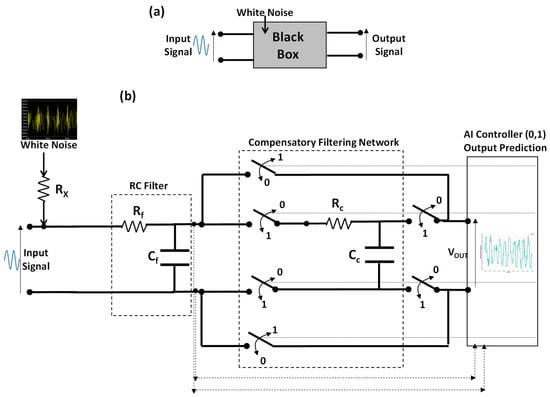
Figure 1.
(a) Black-box model of the network embedding the proposed (b) RC cascade network model (double RC stages) denoising the noisy output signal.
The circuit model is characterized by considering the Rx-parametric analysis simulating the different effects of the white noise at the output port. A first RC low-pass filtering network constituted by the electrical resistance Rf and the capacitance Cf enables the main denoising process (first RC filter stage). Based on the predicted results, an AI controller is able to select only the RC first stage or to further connect in cascade another RC filtering network (compensatory network) constituted by other elements (resistance Rc and capacitance CC) able to improve the final filtering result according with the predicted envelopes of the output voltage. The circuit is modeled by different switches controlled by AI triggering the command ‘0’ to select only the first RC stage, or the command ‘1’ to select the whole cascade network including the compensatory filtering stage. The goal of the proposed model is to use the AI noisy signal prediction to decide the selection of the second RC stage dynamically optimizing the filtering process.
The electrical signals of the circuit model of Figure 1 are estimated by the LTSpice circuit of Figure 2. LTSpice is an open-source ‘SPICE-based’ analog electronic circuit simulator [26] (Version x64: 24.0.12) suitable for time-domain and frequency-domain simulations. The circuit model of Figure 2 takes into account the coupling of white noise with the input signal defined as follows:
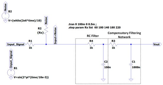
Figure 2.
LTSpice RC cascade network denoising the noisy signal: single RC stage connected to an RC compensatory filtering network (second stage). The symbol ‘*’ indicates a multiplication.
The carrier of Equation (1) is f0 = 100 Hz. The time-domain simulation is performed by setting a transient analysis with the following parameters: stop time = 100 ms, time to start saving data = 0 s, maximum time step = 0.5 ms. The coupling between signal and noise is modulated through the Rx resistance. A parametric analysis versus the variable Rx is performed to analyze the different noise modulation effects: the parametric analysis is executed by assigning the values of Rx as 60 Ω, 100 Ω, 140 Ω, 180 Ω, and 220 Ω. The first RC stage is constituted by the electrical resistance R4 = 1 kΩ and the capacitance C2 = 100 nF as fixed parameters. The second stage behaves as a further compensatory filtering network constituted by other R and C parameters (variable parameters) to assign the function of the predicted trends of the voltage output envelopes (ANN and RF predicted trend). White noise is commonly used to describe a random noisy process as a random process X(t) having a flat power spectral density SX(f):
In the proposed simulations, the white noise intensity is variable and modeled by the Rx resistance of Figure 2 modulating the noise amplitude (parametric simulation changing the Rx value). All electronic and electrical elements intrinsically generate noise which could be modeled by random white noise. The noise for semiconductor devices includes all resistors’ noise effects such as thermal, shot, and avalanche noises. The thermal noise (named the Johnson noise) characterizes all passive resistive elements and is generated by the random Brownian motion of electrons increasing with temperature in electrical resistances. The thermal noise is defined by the following power density:
where vn is the noise voltage (in Volts rms units) which is the value that would be measured driving a totally noise-free band-pass filter (with bandwidth B) with a voltage generated by a resistor at temperature T, KB is the Boltzmann’s constant (expressed in Joules per Kelvin), T is the resistor’s absolute temperature (expressed in Kelvin), R is the resistor’s value (expressed in Ohms), and B = Δf is the band. The shot noise (named the Schottky noise), is generated in active devices for charge flowing as in transistors and diodes. The noise is due to the random arrive of individual electrons flowing through the junction generating microscopic current pulses. This noise can be modeled by a Gaussian white spectral density:
where In is the noise current (in Ampere rms units) estimating the electrical current fluctuations, q is the electron charge (1.6 × 10⁻¹⁹ C), IDC is the direct current (DC), and B = Δf is the band. Finally, the avalanche noise is typical in p-type and n-type (PN) junctions as Zener diodes, working in reverse breakdown mode: the current generated during the avalanche breakdown process is made by random distributed noise spikes behaving as shot noises. In the proposed study, the frequency analysis is performed by means of the fast Fourier transform (FFT) algorithm. All the white noise typologies are characterized by intensity depending on the effective physical effect. In the discussed model, the noise intensities are changed by adding in series to the white noise generator an Rx resistance having the role of modulating the noise amplitude (see Figure 2).
The AI prediction of the noisy signal is implemented by the Konstanz Information Miner (KNIME) workflow of Figure 3. KNIME is an open-source tool [27] adopting graphical interfaces for the setting of the hyperparameters of the AI algorithms. The KNIME workflow is structured into the following three main sequential parts:
- -
- Input data: input dataset for the training and testing of the AI supervised algorithms;
- -
- Data pre-processing: data cleaning and manipulation providing the final dataset to process by the AI algorithms;
- -
- Data processing and reporting: AI data processing, data visualization, and algorithm performance.
The KNIME workflow graphical user interfaces (nodes) are as follows:
- -
- ‘File Reader’: data input importing the output voltages of the parametric analysis (output of the first RC filtering stage) changing with the Rx noise parameter;
- -
- ‘Normalizer’: scaling of the input voltage data from values ranging from 0 to 1 (decrease in the computational error);
- -
- ‘Column Appender’: merging operation of the all input data into an unique data table to be processed by the ANN and RF algorithms;
- -
- ‘Row Filter’: filter preparing the best database to process (the final record number to process is 2409);
- -
- ‘Partitioning’: block able to structure the training and the testing dataset (randomly distributed with 70% in the training dataset and the remaining 30% in the testing dataset);
- -
- ‘RProp MLP Learner’: block implementing an ANN multilayer perceptron (MLP) learning algorithm using the RProp optimizer;
- -
- ‘MultiLayer Perceptron Predictor’: node adopted for the ANN testing data processing;
- -
- ‘Random Forest Learner’: RF algorithm learner block;
- -
- ‘Rando Forest Predictor’: RF algorithm testing block;
- -
- ‘Numeric Scorer’: node estimating algorithm performances;
- -
- ‘Line Plot’: dashboard visualizing ANN and RF results;
- -
- ‘X-Partitioner’: node used for the cross-validation loop; the dataset is divided into different groups named folds (for the specific case, 10 folds are considered);
- -
- ‘X-Aggregator’: at the end of the loop, the ‘X-Aggregator’ node aggregates the results from each iteration; all nodes between the ‘X-Partitioner’ and the ‘X-Aggregator’ node are iteratively executed; the block compares the predicted classes with the real classes for all rows providing iteration statistics.
The protocol defining the denoising process using AI is designed by a Business Process Modeling and Notation (BPMN) workflow (see Section 4). The BPMN is an international standard (ISO/IEC 19510:2013 standard [28]) useful to define all the steps to follow for a measurements and actuation process suitable for the modeling of manufacturing production processes.
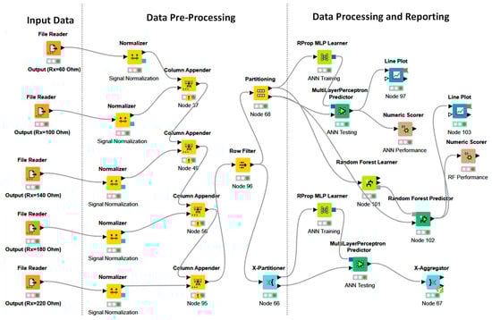
Figure 3.
KNIME workflow adopted for RF and ANN signal prediction.
3. Results
This section proposes three sub-sections: the first describes the white noise effect by adopting the LTSpice simulator; the second discusses the ANN and RF results defining predictive specifications to optimize the filtering process and algorithm efficiency; finally, the third sub-section allows the LTSpice simulator to prove the efficiency of the second filtering stage based on predictive results.
3.1. White Noise and RC Filtering: LTSpice Simulation
The time-domain input signal is plotted in Figure 4a. The FFT signal of Figure 4b highlights the carrier component at f0 = 100 Hz. White noise is added to the input signal following the schemes of Figure 1 and Figure 2. The time-domain white noise signal and the related FFT response are illustrated in Figure 5a,b, respectively.
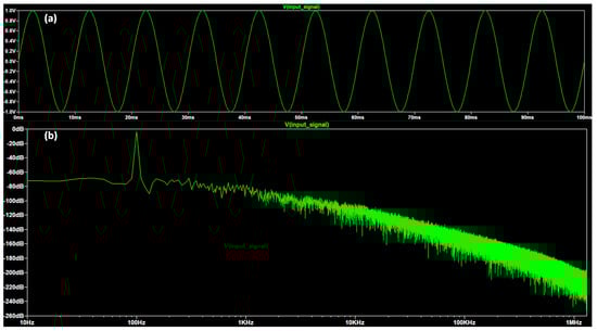
Figure 4.
(a) Time-domain of the pure sinusoidal input signal of Equation (1), and (b) the related FFT spectrum (f0 = 100 Hz).
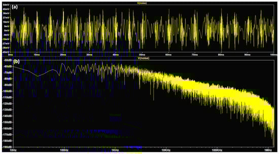
Figure 5.
(a) Time-domain white noise signal and (b) the related FFT spectrum.
The random nature of the noisy signal is observed in Figure 5, where no carriers are observed in a broad band. The white noise influences the input signal, distorting the latter as observed in Figure 6 representing the simulation of a parametric analysis modeling the noise modulation effect: by changing the parameter Rx of the white noise (Rx values of 60 Ω, 100 Ω, 140 Ω, 180 Ω, and 220 Ω), it is possible to observe the ripple behavior intensity, the signal amplitude variation, and the signal shifting. Specifically, for lower values of Rx a greater decrease is observed in the input signal voltage amplitude; otherwise, for a higher value of Rx, a higher value of the input signal voltage amplitude is observed.
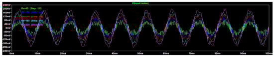
Figure 6.
Rx-parametric analysis of the voltage input influenced by white noise.
The basic circuital behavior of a single RC stage and a double RC stage is described in Appendix A: this study allows us to better comprehend the effect of each electrical component facilitating an understanding of the whole circuit behavior. As observed in Appendix A, the first RC stage, without the noise, generates a slow shifting of the output signal. The effects of the C1 parameter, also in the presence of white noise, are the shifting of the output voltage and the amplitude decrease (the output signal amplitude decreases with an increase in the C1 parameter).
3.2. ANN and RF Noisy Signal Prediction: Predicted Signal Trends and Algorithm Performances
The proposed model is able to learn the ANN and RF supervised algorithms through the output signals of the first RC filtering stage. The learning models allow us to predict the signal voltages at the output of the first filtering stage by considering all the signals (noise plus RC signals) enclosed in a black box. In Figure 7a–d, different comparisons between the voltage outputs (using different RX values) and the ANN predictions are illustrated. The ANN simulations highlight the trend overlapping between the output voltage signal and the predicted ones. We note that for certain noise intensities, the predicted signal trends present differences if compared with those of the output signals: this is due to the learning of the algorithm (history of different signals with different noise intensities) and not to the algorithm performances which appear to be rather good (see Table 1).
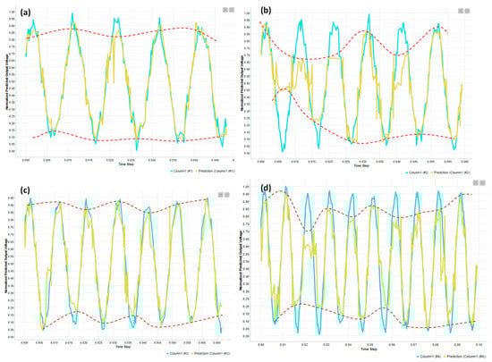
Figure 7.
(a–d) Examples of ANN prediction: upper and lower predicted envelopes (red dashed lines). Simulations considering (a) Rx = 100 Ω (Column 1 (#1)), (b) Rx = 140 Ω (Column 1 (#2)), (c) Rx = 180 Ω (Column 1 (#3)), and (d) Rx = 220 Ω (Column 1 (#4)). The learning model is constructed by considering all the output signals and the related time steps. The partitioning of the dataset is as follows: 70% in the training dataset and 30% in the testing dataset (randomly generated). The electrical parameters considered for the calculus are as follows (see elements in Figure 2): R1 =1 kΩ, R4 =1 kΩ, and C2 = 100 nF.

Table 1.
Comparison between ANN and RF algorithms: MSE and MAE performance parameters. The ANN approach shows a slightly better performance.
The plots of Figure 7 are characterized by different time steps according with the LTSpice sampling. The main result of Figure 7 is the prediction of the noisy signal trend marked by the red dashed lines. The analysis of the envelope trend supports the decision making about the application of the second filtering stage (compensatory filtering network of Figure 2) and the choice of the parameters C1 and R3 of Figure 2 able to optimize the denoising process. The RF results are very similar to ANN ones. In Figure 8, a comparison between the ANN and RF trend of the normalized predicted output voltage is illustrated. The algorithm performance is estimated by the mean absolute error (MAE) and the mean squared error (MSE) defined as follows:
where |yi − xi| = ei is the arithmetic average of the absolute error, yi is the predicted value and xi is the true value, n is the number of the predicted results, Yi is the vector of the observed values, and Ŷi is the vector of the predicted values. The MAE is the absolute deviation between the observed and predicted values. The MSE is the squared deviation between the observed and predicted values. Both the yi and Ŷi values refer to the points of the ANN/RF predictions estimated at precise epochs, while both the xi and Yi values refer to the voltage output considered as the class to predict and estimated at the same epochs (the column containing the target variable).
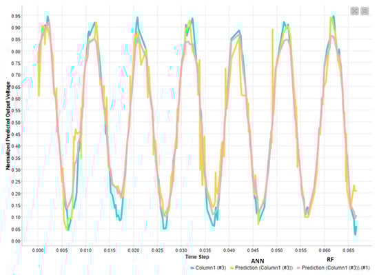
Figure 8.
Comparison between the ANN and RF trend of normalized predicted output voltage (Column 1 (#3) indicates the output normalized voltage). The calculus is performed by considering Rx = 180 Ω. The partitioning of the dataset is as follows: 70% in the training dataset and 30% in the testing dataset (randomly generated).
The method followed to fix the hyperparameters of the ANN algorithm is summarized in the following steps, specifically it is as follows:
- -
- Fix the minimum number of neurons per layer (in the proposed case, the minimum number is 10 corresponding to the number of the input nodes);
- -
- Fix the number of epochs enough to complete the algorithm’s iterations (in the analyzed case the epochs are 400);
- -
- Vary the number of hidden layers, finding the minimum error condition (see Figure 9, finding the minimum condition for 18 hidden layers).
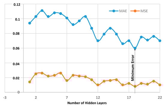 Figure 9. ANN algorithm performance: MAE and MSE errors changing the number of hidden layers.
In Table 1, the performance of the ANN algorithm is compared with the RF one in terms of the MSE and MAE parameters: a slow variation is observed, validating both the ANN and RF approaches for the prediction analysis. In Table 2, the MSE values of the cross-validation test of the ANN algorithm are listed. The cross-validation test is executed for the optimized ANN-MLP algorithm: the test considers ten number of validations adopting the stratified sampling to structure the ten folds. For the analyzed case, the best estimated MSE is 0.008. The similar performance results in Table 2 prove that the adopted dataset is rather balanced and validate the correct choice of the hyperparameters. In Appendix B, the best ANN architecture providing the minimum ANN error is illustrated.
Table 2.
ANN 10-fold cross-validation test: MSE versus the different folds constructed for the testing.
3.3. Denoising Optimization through the Second Compensatory RC Stage
The predicted envelopes of Figure 7 allow the choice of the electrical parameter of the RC compensatory filtering stage of Figure 2: specifically, good parameters for adjusting the signal trend are C1 = 1000 nF and R3 = 1 kΩ. The choice of network parameters is related to the compensation of the predicted worst condition (greater difference between upper and lower envelopes) indicating the worst condition of noise ripple. The LTSpice tool is adopted again to check this compensation.
The simulation of the parametric analysis shows at the output of the first RC stage a noisy signal (see Figure 10a) which is further denoised by the compensatory RC filtering stage, cleaning the final signal (see Figure 10b) and proving the correct choice of the C1 and R3 parameters.
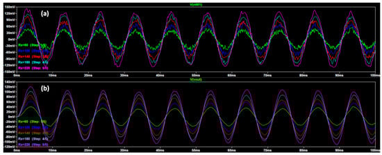
Figure 10.
Parametric analysis versus the Rx: (a) voltage at the output of the first RC stage (noisy signal); (b) output voltage at the end of the compensatory RC filtering stage (denoised signal). The steps indicated in the legend refer to the steps of the parametric analysis (Step 1/5 refers to the parametric analysis considering Rx = 60 Ω, Step 2/5 refers to the parametric analysis considering Rx = 100 Ω, and so on). The considered electrical parameters are as follows (see Figure 2): R1 =1 kΩ, R4 =1 kΩ, C2 = 100 nF, C1 = 1000 nF, and R3 = 1 kΩ.
By observing a predicted voltage amplitude decrease, it is preferable to apply a further corrective action by adding an operational amplifier at the circuit output. Furthermore, a prediction of a signal shift requires a corrective action based on signal shifting (see the phase shift effect in Appendix A). The clearer frequency response behavior of the compensatory network is also observed by the FFT parametric analysis of Figure 11 (Figure 11a,b), showing the parametric frequency responses at the output of the first RC stage and at the end of the compensatory circuit varying Rx, respectively. Figure 11 highlights that the frequency response is also denoised using the compensatory filtering stage (simultaneous check between the time-domain and frequency-domain responses).
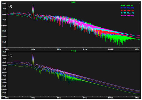
Figure 11.
(a) FFT parametric analysis versus the Rx parameter at the output of the first filtering stage. (b) FFT responses at the output of the compensatory circuit (clearer frequency responses due to a good filtering compensation). The considered electrical parameters are the same as in Figure 10.
4. Discussion
White noise is triggered by random processes involving signal coupling, turbulence or vibration effects, random impacts, electronic defects, or electromagnetic interferences due to charge/discharge processes in a motor, cabling, electrical/electronic junctions, etc., and it particularly occurs in machinery control systems. White noise generalizes the presence of noisy sources which are not easy to identify. For this purpose, the proposed black-box model is suitable not to classify the noise type but to predict the output signal trend of a specific machinery environment affected by disturbances. The application of the proposed model with random noise as white noise allows us to generalize the application field for different typologies of noises including those with carrier components and additive or multiplicative noises.
The white noise and AI implementation are characterized by different advantages and disadvantages as listed in Table 3. Specifically, Table 3 addresses the proposed modeling in different methodologies of analysis such as generic signal processing, time-series analysis, statistics, interference analysis, machine control systems, and Digital Twin (DT) simulations, by highlighting possible advantages and disadvantages of implementing white noise.
Table 3.
Advantages and disadvantages of the white noise and AI implementations.
The limitations of the proposed approach are mainly in the use of passive RC circuits. Possible future developments could be in the design of a similar filtering network using the same procedure as the proposed paper but adopting active elements. In Table 4, these aspects are detailed.
Table 4.
Limitations and perspectives of the proposed approach.
The proposed data processing model is a good alternative to non-AI methods such as the overall filtering algorithm [43], Weighted Nuclear Norm Minimization (WNNM) [44], the Unbiased Finite Impulse Response (UFIR) filtering algorithm [45], the Mixed Gaussian and Random-Valued Impulse Noise (RVIN) removal approach [46], and the bias compensated Maximum Complex Correntropy Criterion (MCCC) [47].
The protocol indicating the usage of the proposed methodology is illustrated in the BPMN workflow of Figure 12. The workflow is described by the following steps numbered in the figure:
- -
- Step 1: the first RC stage is able to read possible noisy voltage outputs; the outputs are adopted for the AI training and testing processes (creation of the historical dataset);
- -
- Step 2: ANN/RF predictions provide the envelopes of the predicted voltages and the predicted signal trend;
- -
- Step 3b: if the envelopes are regular, no further filtering is required and the machine is correctly controlled (the ‘0’ command of the circuit of Figure 1);
- -
- Step 3a/Step 4a: if the envelopes are different from the expected voltage envelopes (voltage envelopes without the noise effect), then the circuit simulation is executed to find the best R and C component of the second stage filtering compensatory network (Step 3a); the best R and C components are selected dynamically, and the further compensatory RC filtering network is applied (the ‘1’ command of the circuit of Figure 1).
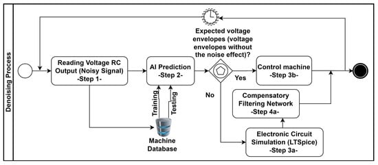
Figure 12.
BPMN workflow of the guidelines for the use of the circuit model of Figure 1.
The proposed work is a full upgrade of a previous work [13] adopting AI in electronic systems. The main differences and novelties are in the functionalities listed in Table 5.
Table 5.
Functionalities and novelties of the proposed model compared with the functionalities of [13].
In Appendix C, an example is described of the application of the ANN model considering experimental data [48]. The proposed model is a first step to realize a real testbed Digital twin (DT) including as hardware a microcontroller, and as software we use an interface implementing the workflow of Figure 12. A scheme of the testbed architecture is illustrated in Figure 13.
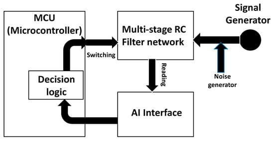
Figure 13.
DT testbed architecture.
5. Conclusions
The paper investigates an innovative approach to filter generic white noise disturbing a control signal. Specifically, a double RC stage network is able to filter into one or two steps a sinusoidal control signal based on the predicted envelopes of the voltage outputs. Specifically, ANN and RF supervised algorithms have been applied to predict the output voltage trend. The SPICE-based circuit model allowed us, through a parametric analysis, to understand the RC output behavior simulating the noise modulation effect by means of a resistance element. Based on the output trend, the proposed model is able to intelligently select or not select a further compensatory RC filtering second stage optimizing the denoising process. Specifically, the AI model optimizes the choice of the resistance and capacitance values of the second filtering stage according with the predicted voltage output. Furthermore, the AI prediction provides further information about other possible corrective actions introducing other circuital elements to achieve signal gaining or response shifting. As for practical applications in industrial environments influenced by random noises, the black-box model is the best choice to parametrically simulate the output signals when different modulation effects of the white noise are considered and to efficiently train the machine-learning algorithms. Finally, the paper defines by a BPMN workflow the guidelines to use for the proposed model of the denoising filtering process. The whole discussed model is addressed in Industry 5.0 application fields including advanced manufacturing control systems requiring signal denoising. The model is adaptable to other typologies of electronic filtering stages such as active filters and a higher order of low-pass, band-pass, and high-pass filters. The purpose of the proposed research is to define a methodological procedure structuring a filtering Digital Twin (DT) model suitable for the automatic denoising process by means of circuit and AI simulations.
The main novelties of the research are the modeling of a generic white noise effect applicable to generic electronic circuits including multi-stage filtering networks able to improve the noise filtering. The implementation of the pseudocode implementing the AI controller automatism is under investigation and will be the subject of a further publication. Future works will also be addressed on the implementation of the automatic control providing the switching commands of the proposed network.
Funding
This research received no external funding.
Data Availability Statement
Data are included in the paper.
Conflicts of Interest
The author declares no conflicts of interest.
Appendix A
Figure A1 illustrates the time-domain and the frequency response of a single RC filtering stage without white noise.
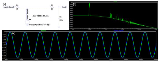
Figure A1.
(a) LTSpice circuit of a single RC stage without considering the white noise. (b) Output FFT response. (c) Time-domain input and output signals showing a signal little shift. The electrical parameters of the simulated circuit of (a) are as follows: R1 = 1 kΩ, R4 = 1 kΩ, and C2 = 100 nF.
Figure A2 shows the time-domain and the frequency response of a double-stage RC filters without white noise.
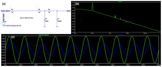
Figure A2.
(a) LTSpice circuit of a double RC filtering stage without considering the white noise. (b) Output FFT response. (c) Time-domain input and output signals showing a shift and an amplitude decrease. The electrical parameters of the simulated circuit of (a) are as follows: R1 = 1 kΩ, R4 = 1 kΩ, C2 = 100 nF, Ω, R3 = 1 kΩ, and C1 = 1000 nF.
Figure A3 shows the time-domain and the frequency response of a single stage RC filter with white noise and changing the C1 parameter.
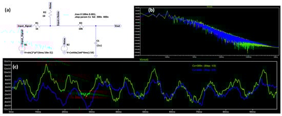
Figure A3.
(a) LTSpice circuit of a single RC filtering stage by considering the white noise as a disturbance. (b) Output FFT response. (c) Time-domain input and output signals showing a little shift and an amplitude decrease when changing the C1 parameter (a signal amplitude decrease is observed with an increase in C1 from 300 nF to 400 nF). The electrical parameters of the simulated circuit of (a) are as follows: R1 = 1 kΩ, R2 = 10 kΩ, R3 = 10 kΩ, and C1 = 300 nF and 400 nF (parametric analysis).
Appendix B
The ANN network providing the best performance is sketched in Figure A4. The network is defined by the following parameters: 10 input nodes (output of the first stage of the RC filters and related time steps ranging from 0.0002 ms to 0.0019 ms, and storing the voltage signal trends), 10 neurons per layer, 18 hidden layers, and the epoch number (time steps of the ANN iterations) equals 400. The output nodes are the five predicted signals corresponding to each output voltage (Vout# signal). Figure A5 illustrates an example of voltage sampling.
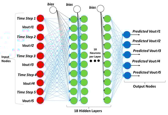
Figure A4.
Optimized ANN deep learning architecture adopted in the proposed paper. The voltages output signals (Vout# signals) are estimated considering the parametric analysis with different Rx values (60 Ω, 100 Ω, 140 Ω, 180 Ω, and 220 Ω).
Figure A5.
Example of voltage sampling of the parametric analysis for each output voltage (Vout# signal). The sampling is automatically carried out by the LTSpice tool fixing a maximum time step of 0.5 ms.
Appendix C
The AI model is applied to a practical case regarding a radio frequency attack in cybersecurity application fields [48]. The ANN model is applied to the radio frequency signal, proving that the ANN algorithm is suitable for any kind of applications matching Industry 5.0 scenarios. In Figure A6, a comparison is illustrated between an RF wireless transmitted signal and the ANN prediction one observing a good matching with the periodic trend. The ANN is also suitable to approximately predict the trend of very noisy signals (peak position trend) as shown in Figure A7, thus proving that the white noise approach is suitable for generic applications of noisy environments.
Figure A6.
ANN prediction of the radio frequency normalized signal [48].
Figure A7.
ANN prediction of a fully noisy radio frequency voltage signal [48].
References
- Haas, R.; Lukachev, E.; Scheidl, R. An RC Filter for Hydraulic Switching Control with a Transmission Line Between Valves and Actuator. Int. J. Fluid Power 2014, 15, 139–151. [Google Scholar] [CrossRef]
- Mondal, C.; Azam, M.K.; Ahmad, M.; Hasan, S.M.K.; Islam, M.R. Design and Implementation of a Prototype Electrooculography Based Data Acquisition System. In Proceedings of the 2015 International Conference on Electrical Engineering and Information Communication Technology (ICEEICT), Savar, Bangladesh, 21–23 May 2015; IEEE: Piscataway, NJ, USA; pp. 1–6. [Google Scholar]
- Oshima, T.; Maio, K.; Hioe, W.; Shibahara, Y.; Doi, T. Automatic Tuning of RC Filters and Fast Automatic Gain Control for CMOS Low-IF Transceiver. In Proceedings of the IEEE 2003 Custom Integrated Circuits Conference, San Jose, CA, USA, 24 September 2003; pp. 5–8. [Google Scholar]
- Jin, G.; Wu, H.; Yin, Y.; Zheng, L.; Zhuang, Y. A High-Accuracy RC Time Constant Auto-Tuning Scheme for Integrated Continuous-Time Filters. Micromachines 2024, 15, 166. [Google Scholar] [CrossRef] [PubMed]
- Ramos, G.A.; Costa-Castelló, R. Energy Management Strategies for Hybrid Energy Storage Systems Based on Filter Control: Analysis and Comparison. Electronics 2022, 11, 1631. [Google Scholar] [CrossRef]
- Salari, O.; Zaad, K.H.; Bakhshai, A.; Jain, P. Filter Design for Energy Management Control of Hybrid Energy Storage Systems in Electric Vehicles. In Proceedings of the 2018 9th IEEE International Symposium on Power Electronics for Distributed Generation Systems (PEDG), Charlotte, NC, USA, 25–28 June 2018; IEEE: Piscataway, NJ, USA; pp. 1–7. [Google Scholar]
- Lau, L. Wavelet Packets Based Denoising Method for Measurement Domain Repeat-Time Multipath Filtering in GPS Static High-Precision Positioning. GPS Solut. 2017, 21, 461–474. [Google Scholar] [CrossRef]
- Alizadeh, M.; Moghaddam, M.M.; HosseinNia, S.H. A Novel Zero Delay Low Pass Filter: Application to Precision Positioning Systems. ISA Trans. 2021, 111, 231–248. [Google Scholar] [CrossRef] [PubMed]
- Sun, Y.; Tang, X.; Sun, X.; Jia, D.; Cao, Z.; Pan, J.; Xu, B. Model Predictive Control and Improved Low-Pass Filtering Strategies Based on Wind Power Fluctuation Mitigation. J. Mod. Power Syst. Clean Energy 2019, 7, 512–524. [Google Scholar] [CrossRef]
- Magsi, H.; Sodhro, A.H.; Chachar, F.A.; Abro, S.A.K. Analysis of Signal Noise Reduction by Using Filters. In Proceedings of the 2018 International Conference on Computing, Mathematics and Engineering Technologies (iCoMET), Sukkur, Pakistan, 3–4 March 2018; pp. 1–6. [Google Scholar]
- Kelemenová, T.; Benedik, O.; Koláriková, I. Signal Noise Reduction and Filtering. Acta Mechatronica 2020, 5, 29–34. [Google Scholar] [CrossRef]
- Yu, F.-M.; Lee, K.-C.; Jwo, K.-W.; Chang, R.-S.; Lin, J.-Y. Low Distortion of Noise Filter Realization with 6.34 V/μs Fast Slew Rate and 120 mVp-p Output Noise Signal. Sensors 2021, 21, 1008. [Google Scholar] [CrossRef] [PubMed]
- Massaro, A. ANNs Predicting Noisy Signals in Electronic Circuits: A Model Predicting the Signal Trend in Amplification Systems. AI 2024, 5, 533–549. [Google Scholar] [CrossRef]
- Lai, W.-C.; Jian, R.; Xin, X. Noise Suppression of Artificial Intelligence Filter for Radio Frequency Interference. In Proceedings of the 2020 IEEE International Conference on Consumer Electronics—Taiwan (ICCE-Taiwan), Taoyuan, Taiwan, 28–30 September 2020; IEEE: Piscataway, NJ, USA; pp. 1–2. [Google Scholar]
- Pu, S.; Zhang, H.; Mao, C.; Yang, G. A Classification Based on Random Forest for Partial Discharge Sources. In Proceedings of the 2021 33rd Chinese Control and Decision Conference (CCDC), Kunming, China, 22–24 May 2021; IEEE: Piscataway, NJ, USA; pp. 2307–2311. [Google Scholar]
- Zhao, T.; Wei, J.; Lan, B.; Peng, Q.; Wan, J. A Unified Black-box Macro Model for Analog Circuit Based on Artificial Neural Network. Int. J. Circuit Theory Appl. 2023, 51, 4455–4464. [Google Scholar] [CrossRef]
- Zhou, H.; Chen, W.; Shen, C.; Cheng, L.; Xia, M. Intelligent Machine Fault Diagnosis with Effective Denoising Using EEMD-ICA- FuzzyEn and CNN. Int. J. Prod. Res. 2023, 61, 8252–8264. [Google Scholar] [CrossRef]
- Miao, F.; Zhao, R.; Wang, X. A New Method of Denoising of Vibration Signal and Its Application. Shock Vib. 2020, 2020, 7587840. [Google Scholar] [CrossRef]
- Song, J.; Yu, Y.; Chen, L. Research on Adaptive DE-Noising Technique for Time-Domain Reflectometry Signal Based on Wavelet Analysis. In Advanced Research on Electronic Commerce, Web Application, and Communication; Springer: Berlin/Heidelberg, Germany, 2011; pp. 127–132. [Google Scholar]
- Dong, W.; Ding, H. Full Frequency De-Noising Method Based on Wavelet Decomposition and Noise-Type Detection. Neurocomputing 2016, 214, 902–909. [Google Scholar] [CrossRef]
- Polimi.it. Available online: https://www.politesi.polimi.it/retrieve/1ab16241-5240-4ee5-8251-330d7508506b/Executive_Summary-Daniele_De_Dominicis.pdf (accessed on 2 June 2024).
- Ruppert, T.; Abonyi, J. Software Sensor for Activity-Time Monitoring and Fault Detection in Production Lines. Sensors 2018, 18, 2346. [Google Scholar] [CrossRef] [PubMed]
- Suawa, P.F.; Halbinger, A.; Jongmanns, M.; Reichenbach, M. Noise-Robust Machine Learning Models for Predictive Maintenance Applications. IEEE Sens. J. 2023, 23, 15081–15092. [Google Scholar] [CrossRef]
- Sastry Vedam, R.; Sarma, M.S. Power Quality: VAR Compensation in Power Systems: Var Compensation in Power Systems; CRC Press: Boca Raton, FL, USA, 2008. [Google Scholar]
- Wilamowski, B.M.; David Irwin, J. Fundamentals of Industrial Electronics; CRC Press: Boca Raton, FL, USA, 2018. [Google Scholar]
- LTspice. Available online: https://www.analog.com/en/resources/design-tools-and-calculators/ltspice-simulator.html (accessed on 7 June 2024).
- KNIME. Available online: https://www.knime.com/ (accessed on 10 June 2024).
- ISO/IEC 19150:2013; Information Technology—Object Management Group Business Process Model and Notation. ISO: London, UK, 2013. Available online: https://www.iso.org/standard/62652.html (accessed on 27 July 2024).
- Arumugam, S. Investigations on Using White Noise as a Test Signal for Performing Frequency Response Measurements on Transformers. Electr. Power Syst. Res. 2022, 202, 107586. [Google Scholar] [CrossRef]
- Baskys, A. A Combined Controller for Closed-Loop Control Systems Affected by Electromagnetic Interference. Sensors 2024, 24, 1466. [Google Scholar] [CrossRef] [PubMed]
- Saponaro, A.; Dipierro, G.; Cannella, E.; Panarese, A.; Galiano, A.M.; Massaro, A. A UAV-GPR Fusion Approach for the Characterization of a Quarry Excavation Area in Falconara Albanese, Southern Italy. Drones 2021, 5, 40. [Google Scholar] [CrossRef]
- Starace, G.; Tiwari, A.; Colangelo, G.; Massaro, A. Advanced Data Systems for Energy Consumption Optimization and Air Quality Control in Smart Public Buildings Using a Versatile Open Source Approach. Electronics 2022, 11, 3904. [Google Scholar] [CrossRef]
- Massaro, A. Advanced Electronic and Optoelectronic Sensors, Applications, Modelling and Industry 5.0 Perspectives. Appl. Sci. 2023, 13, 4582. [Google Scholar] [CrossRef]
- Lay-Ekuakille, A.; Massaro, A.; Singh, S.P.; Jablonski, I.; Rahman, M.Z.U.; Spano, F. Optoelectronic and Nanosensors Detection Systems: A Review. IEEE Sens. J. 2021, 21, 12645–12653. [Google Scholar] [CrossRef]
- Zhang, Z.; Chen, S.; Zhou, Z.; Li, H. An Active Noise Control System Based on Reference Signal Decomposition. Digit. Signal Process. 2022, 129, 103676. [Google Scholar] [CrossRef]
- Singh, D.; Gupta, R.; Kumar, A.; Bahl, R. Attention Based Convolutional Neural Network for Active Noise Control. In Proceedings of the 2024 The 8th International Conference on Machine Learning and Soft Computing, Singapore, 26–28 January 2024; ACM: New York, NY, USA, 2024. [Google Scholar]
- Luo, Z.; Shi, D.; Shen, X.; Gan, W.-S. Unsupervised Learning Based End-to-End Delayless Generative Fixed-Filter Active Noise Control. arXiv 2024, arXiv:2402.09460. Available online: https://arxiv.org/html/2402.09460v1 (accessed on 23 June 2024).
- Mylonas, D.; Erspamer, A.; Yiakopoulos, C.; Antoniadis, I. A Virtual Sensing Active Noise Control System Based on a Functional Link Neural Network for an Aircraft Seat Headrest. J. Vib. Eng. Technol. 2024, 12, 3857–3872. [Google Scholar] [CrossRef]
- Cvetanovic, R.; Petric, I.Z.; Mattavelli, P.; Buso, S. Switching Noise Propagation and Suppression in Multisampled Power Electronics Control Systems. IEEE Trans. Power Electron. 2024, 39, 149–163. [Google Scholar] [CrossRef]
- Monjur, M.M.R.; Heacock, J.; Calzadillas, J.; Mahmud, M.D.S.; Roth, J.; Mankodiya, K.; Sazonov, E.; Yu, Q. Hardware Security in Sensor and Its Networks. Front. Sens. 2022, 3, 850056. [Google Scholar] [CrossRef]
- Monjur, M.R.; Sunkavilli, S.; Yu, Q. ADobf: Obfuscated Detection Method against Analog Trojans on I2C Master-Slave Interface. In Proceedings of the 2020 IEEE 63rd International Midwest Symposium on Circuits and Systems (MWSCAS), Springfield, MA, USA, 9–12 August 2020; pp. 1064–1067. [Google Scholar]
- Monjur, M.; Calzadillas, J.; Yu, Q. Hardware Security Risks and Threat Analyses in Advanced Manufacturing Industry. ACM Trans. Des. Automat. Electron. Syst. 2023, 28, 1–22. [Google Scholar] [CrossRef]
- Ren, Y.; Li, T.; Xu, J.; Hong, W.; Zheng, Y.; Fu, B. Overall Filtering Algorithm for Multiscale Noise Removal from Point Cloud Data. IEEE Access 2021, 9, 110723–110734. [Google Scholar] [CrossRef]
- Li, J.; Fan, W.; Li, Y.; Qian, Z. Low-Frequency Noise Suppression in Desert Seismic Data Based on an Improved Weighted Nuclear Norm Minimization Algorithm. IEEE Geosci. Remote Sens. Lett. 2020, 17, 1993–1997. [Google Scholar] [CrossRef]
- Zhao, S.; Shmaliy, Y.S.; Ahn, C.K.; Liu, F. Self-Tuning Unbiased Finite Impulse Response Filtering Algorithm for Processes with Unknown Measurement Noise Covariance. IEEE Trans. Control Syst. Technol. 2021, 29, 1372–1379. [Google Scholar] [CrossRef]
- Xing, M.; Gao, G. An Efficient Method to Remove Mixed Gaussian and Random-Valued Impulse Noise. PLoS ONE 2022, 17, e0264793. [Google Scholar] [CrossRef] [PubMed]
- Dong, F.; Qian, G.; Wang, S. Bias-Compensated MCCC Algorithm for Widely Linear Adaptive Filtering with Noisy Data. IEEE Trans. Circuits Syst. II Express Briefs 2020, 67, 3587–3591. [Google Scholar] [CrossRef]
- RF Jamming Dataset. Available online: https://www.kaggle.com/datasets/daniaherzalla/radio-frequency-jamming (accessed on 12 July 2024).
Disclaimer/Publisher’s Note: The statements, opinions and data contained in all publications are solely those of the individual author(s) and contributor(s) and not of MDPI and/or the editor(s). MDPI and/or the editor(s) disclaim responsibility for any injury to people or property resulting from any ideas, methods, instructions or products referred to in the content. |
© 2024 by the author. Licensee MDPI, Basel, Switzerland. This article is an open access article distributed under the terms and conditions of the Creative Commons Attribution (CC BY) license (https://creativecommons.org/licenses/by/4.0/).