Time-Delay Estimation Improves Active Disturbance Rejection Control for Time-Delay Nonlinear Systems

Abstract

Lately, active disturbance rejection control (ADRC), a model-independent controller, has become popular for combating various forms of uncertain disturbances incurred in industrial applications. ADRC was validated for external disturbances, internal disturbances, and nonlinearities incurred under realistic scenarios. Time delay challenges all controllers, especially when it coexists with nonlinearities. This paper investigates the impacts of time delay and backlash-like hysteresis nonlinearity in ADRC-controlled systems. These impacts are analyzed, as in the case study, in two ADRC-based methods, namely the ADRC with delayed input method and the predictive extended state observer (PESO)-based ADRC (PESO-ADRC) method. To improve the system response and to attain a decent attenuation of uncertainties, the time-delay estimation (TDE) mechanism is introduced to the concerned ADRC-based methods. Experimental studies are conducted to verify the effectiveness and stability of the proposed TDE-ADRC methods. The results demonstrate the robustness and decent recovery of the transient response after the adverse impact of the backlash-like hysteresis on both concerned ADRC-controlled systems.

1. Introduction

Various disturbance rejection mechanisms have recently gained popularity owing to the impacts of different uncertainties and nonlinearities on real-world systems. Such uncertainties include unmodeled dynamics, time delay, parametric variations, external disturbances, and other nonlinearities that greatly influence the stability and system performance undesirably. Hence, this behavior necessitates estimating and compensating for such intermittences in control systems theory. One such method that forms an effective disturbance rejection mechanism is active disturbance rejection control (ADRC), which is independent of the model of the system to be controlled [1].

The ADRC was first introduced by Han in 1995 [2] and further implemented by Gao [1]. To adhere to the foundation of modern control theory, Han used the basic principle of the PID controller, pertaining to eliminating errors. Hence, ADRC was formally proposed as an effective controller to provide solutions to complex, nonlinear, and time-varying systems. Further, the ADRC can actively estimate internal and external disturbances collectively termed ‘total disturbance’, followed by compensating these total disturbance effects in real-time using the feedback loop. This is achieved with the help of an extended state observer (ESO) that forms an imminent part of the ADRC controller [2].

The internal disturbances include parametric variations (system parameter perturbations) and unmodeled system dynamics [3]. In contrast, external disturbances constitute various uncertainties, such as system input and output disturbances, sensor noise, and nonlinearities like time delay and hysteresis [4]. Therefore, to counteract the impacts of various forms of uncertainty, the ESO subsystem has been modified over time to suit the ADRC operation in various industrial applications such as power electronics [5,6], robotic systems [7], thermal processes [8], microgrids [9], and teleoperation systems [10,11].

Nonlinearity persists in a control system due to the nature of specific electrical or mechanical components present in the system or the interaction of nonlinear components with the environment. A few fundamental techniques for handling the nonlinearity phenomenon were developed, including nonlinear disturbance compensation and feedback linearization [12]. The former relies on an accurate model of the disturbances. However, as real-world systems usually do not have such exact models available, the former technique is often not feasible. Conversely, the latter method can function with appropriate designs irrespective of the actual system model or nonlinear behavior; thus, it is widely considered. Other compensation methods include inversion-based models, which are associated with complexities of calculations and design application [12,13], and some of the latest neural network (NN) methods were developed [14,15,16]. The ADRC controller was designed suitably to estimate and compensate for the nonlinear effects on the system response as the total disturbance.

Moreover, time delay is unavoidable in the communication channel of a given controlled system, such as when transmitting signals over the internet protocol. Further, delays can also exist in system components such as sensors, controlled objects (plants), or actuators. Hence, the existence of a time delay has an adverse impact on the controller’s performance concerning significant oscillatory response and an increase in system response overshoot, thus driving the closed-loop system to instability. Such effects realized the need to design a controller to obtain a decent trade-off between controller operation and disturbance rejection under time-delay control. Though the ADRC controller performs well for various forms of nonlinear disturbance compensation, overcoming the effects due to the present time delay is still challenging. Therefore, estimating and compensating for the effects of time delay is a work in progress for ADRC-based methods [17,18].

1.1. Related Work

This section briefly explains relevant ADRC methods proposed in the literature. Further, a brief overview of control schemes, including the ADRC and the time-delay estimation (TDE) mechanism, has been revisited, highlighting their significance in compensating disturbances and nonlinearities.

In literature [17], popularly used predictive ADRC methods such as the Smith predictor (SP)-based ADRC, extended state predictor observer (ESPO)-based ADRC [19], polynomial predictor (PP)-based ADRC [20], and delayed input-based ADRC [21] were analyzed based on time delay and disturbance compensation criteria. Moreover, predictive ADRC methods are investigated using internal mode control (IMC) interpretations [22]. The results indicated that predictor observer-based ADRC (PO-ADRC) outperformed the other ADRC compensation methods under time-delay control, but further parameter fine-tuning is required to obtain improved system performance. Further, a predictive ESO-based ADRC (PESO-ADRC) method introduced in [23] showed decent robustness to system input and output disturbances and noise in the vicinity of time delay. Furthermore, existing time-delay related ADRC works, such as literature [17,18], dealt with uncertain systems with input time delay. However, further work is needed to analyze the nonlinearity, such as backlash-like hysteresis under time delay and external disturbances present in the concerned systems.

In addition to the time delay and disturbance compensation methods available in the literature, TDE-based methods are presented to combat the concerned system uncertainties and obtain improved system response. TDE, as an estimation method, primarily uses the system’s delayed dynamics to estimate the unknown dynamics of the controlled system [24,25,26]. Time delay control (TDC) forms a subclass of the TDE mechanism, which has created one of the most appropriate and successful compensating methods for systems with nonlinearities and unknown system dynamics [24].

For instance, TDE with a fuzzy PID controller enhanced the controller performance by simplifying the PID tuning process for a robotic manipulator [27]. Further, another PID with a TDE approach [28] leveraged the better controller performance of an adaptive PID controller using gain adaptation in the frequency domain. Furthermore, in another strategy, adaptive robust and nonsingular fast terminal sliding mode controller (SMC) methods based on TDE mechanisms have been developed for robotic manipulators and cable-driven robots [29,30,31], where the backlash hysteresis and complex lumped uncertainties were analyzed, followed by attenuating their negative impacts on system performance. However, future studies will further analyze noise curtailment, chattering effects, saturation, and dead zones. Moreover, in the literature [32], an ADRC controller uses the TDE interpretation with the ESO in the frequency domain to estimate and compensate for the all-clamped plate system’s nonlinearities. However, the study of the external disturbances acting on the system forms part of future studies. Consequently, this article’s main experimental findings focus on improving the recently proposed PESO-ADRC method [23] and the previously developed ADRC with delayed input method [21] in terms of compensation of nonlinearity (backlash-like hysteresis, parameter perturbation, and external disturbance) under time-delay presence, which is explained in the sections to follow.

1.2. Paper Contribution

This paper’s main contribution focuses on improving the PESO-ADRC system’s transient response concerning the nonlinearity introduced in the controlled system, followed by its attenuation. In this context, the nonlinearity referred to is the Duhem backlash-like hysteresis model. The predictive nature of the PESO-ADRC allows it to predict the unknown system dynamics created during the delay and compensate for them as a disturbance under time-delay control. To the best of the author’s knowledge, no prior ADRC study has addressed the suggested approach, which integrates the predictive ADRC-based controller design with a TDE mechanism to effectively compensate for the nonlinearities present in time-delay systems. Hence, it is seen that the TDE mechanism assists in further enhancing the ESO’s disturbance rejection capacity in an ADRC-controlled system. Therefore, this paper introduces the TDE mechanism to the ADRC methods [21,23], to better estimate and reject uncertainties and nonlinearity.

The remainder of the paper is organized as follows: Section 2 highlights the mathematical preliminaries and system descriptions. Section 3 integrates the TDE mechanism with the ADRC methods (with delayed input and the predictive ESO). Section 4 presents experimental analysis and discussions to prove the validity of the proposed TDE-ADRC methods. Finally, conclusions and future recommendations are provided in Section 5.

2. Mathematical Preliminaries and System Description

This section presents a brief overview of the Duhem backlash-like hysteresis model, the object or plant to be controlled, the TDE mechanism, and the concerned ADRC-based controllers.

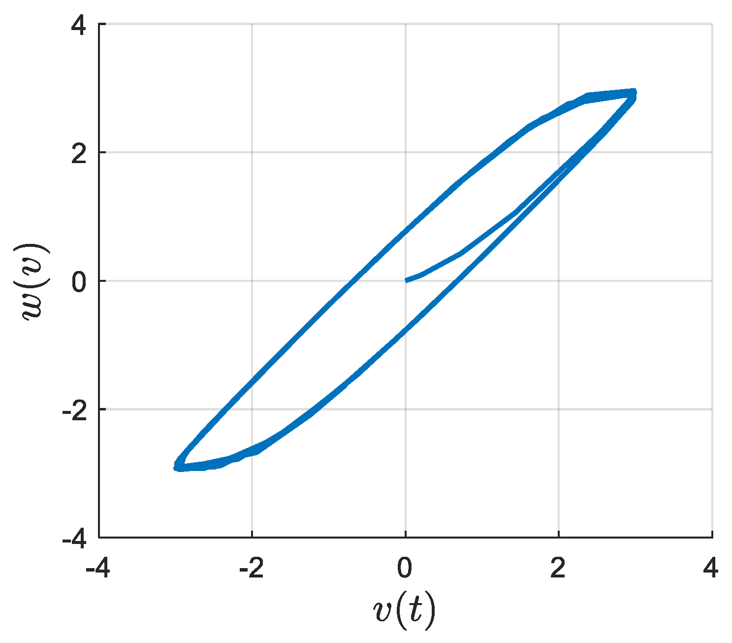
2.1. Duhem Backlash-Like Hysteresis Mathematical Model

It is widely recognized that the hysteresis effect can hinder the precision of both closed-loop and open-loop control systems and cause oscillations to persist. In this paper, the Duhem model was projected for active hysteresis, with its evolution provided in [33,34]. The mathematical representation of the Duhem backlash-like hysteresis model is based on the differential equation given in Equation (1), which emphasizes how an input signal’s change in direction can cause an output signal’s behavior to shift.

$${\displaystyle \frac{dw\left(v\right)}{dx}}=\gamma \left|{\displaystyle \frac{dv}{dt}}\right|\left(\alpha v-w\left(v\right)\right)+\beta {\displaystyle \frac{dv}{dt}}$$

(1)

where $\gamma$, $\alpha ,$ and $\beta$ are constants such that $\gamma >0$ and $\alpha >\beta$. The properties of Equation (1) are detailed in [33]. Equation (1) can be solved to re-express it as given in Equation (2):

$$w\left(v\right)=\alpha v\left(t\right)+\left[w_0-\alpha v_0\right]e^{-\gamma \left(v-v_0\right)\mathrm{s}\mathrm{i}\mathrm{g}\mathrm{n}\left(\dot{v}\right)}+e^{-\gamma v\mathrm{s}\mathrm{i}\mathrm{g}\mathrm{n}\left(\dot{v}\right)}{\int }_{v_0}^v(\beta -\alpha )e^{-\gamma \epsilon \mathrm{s}\mathrm{i}\mathrm{g}\mathrm{n}\left(\dot{v}\right)}d\epsilon$$

(2)

where the initial values of the hysteresis input and output are given by $v_0$ and $w_0,$ respectively. Figure 1 depicts a typical Duhem backlash-like hysteresis characteristic response for γ = 1, α = 1.16, and β = 0.35. Consider the input signal $v\left(t\right)=\rho \sin (2.5t)$, for $\rho$ = 3, and the initial values $v_0=0$ and $w_0$ = 0.

2.2. System Description

In control theory, higher-order systems are commonly analyzed using low-order (typically second-order) approximations, so most controllers concentrate on simpler or lower-order models for real systems for the sake of simplicity and robustness of the resulting control. In this study, the second-order control system model is represented by the state-space form in Equation (3):

$$\left\{\begin{array}{l}\dot{x}\left(t\right)=Ax\left(t\right)+Bu\left(t\right)+\delta \left(x\left(t\right),t\right)\\ y\left(t\right)=C^{T}x\left(t-\tau \right)\\ x\left(0\right)=[{\begin{array}{cc}0& 0\end{array}]}^T\end{array}\right.$$

(3)

where $x\left(t\right)=[{x_1\left(t\right),x_2\left(t\right)]}^T$ and $y\left(t\right)$ are the system state vector and system output, respectively. The given system is subjected to total uncertainties given by $\delta \left(x\left(t\right),t\right),$ and $u\left(t\right)$ is the control input. $\tau$ is the system time delay, and $A$, $B$, and $C$ specify the state-transition, input, and output matrices of the system plant, respectively. The total disturbance $\delta \left(x\left(t\right),t\right)$ includes various disturbances due to unknown system dynamics, parameter perturbation, external disturbance, nonlinearity, and noise acting on the system.

2.3. Time-Delay Estimation Mechanism

TDE is a method for estimating system uncertainties using time-delayed information from the prior sampling event. As seen in Equation (4), the TDE technique introduces a small time delay, called the sampling period, represented by ‘$∆t$’ when designing a controller [25]. By doing so, the TDE diminishes the effect of additive disturbances as a total disturbance.

$$\widehat{\rho }\left(t\right)=\rho (t-∆t)$$

(4)

where the time-delayed value is indicated by the subscript ($t-∆t$). $\widehat{\rho }\left(t\right)$ is the estimation of $\rho \left(t\right)$ and denotes all uncertainties, such as hysteresis, noise, external disturbances, and so on. Thus, the complete TDE law is given in Equation (5),

$$\rho \left(t-∆t\right)=u\left(t-∆t\right)-{\rm N}\ddot{\theta }(t-∆t)$$

(5)

where ${\rm N}$ is a known constant, called the nominal value or a positive diagonal matrix (in the case of multiple input and multiple output (MIMO) systems, such as robotic systems), which is tuned to attain an optimal controller operation. $\ddot{\theta }(t-∆t)$ is the delayed system output dynamics (the second-order deviation), such as the joint position vector for a robotic system.

2.4. ADRC with Delayed Input System

The three main components of an ADRC are the tracking differentiator (TD), the nonlinear state error feedback (NLSEF) controller, and the ESO [1]. Figure 2 showcases the structure of ADRC with delayed input [21], and Figure 3 depicts the PESO-based ADRC structure [23]. The ESO is a vital subsystem of the ADRC that performs active estimation and compensation of the total disturbance ($\delta \left(t\right)$) acting on the controlled object (seen in Equation (3)). In both systems in Figure 2 and Figure 3, with an estimated derivative signal, the TD generates a softer signal. The NLSEF generates the control law $u_0$ by obtaining the difference signals $e_1$ and $e_2$ from the TD-generated signals $v_1\left(t\right)$ and $v_2\left(t\right)$ and the ESO-generated estimated system states $z_1$ and $z_2$. Both the ADRC with delayed input (Figure 2) and the PESO-ADRC (Figure 3) have the same TD and NLSEF, as shown in Equations (6) and (7), respectively.

$$\left\{\begin{array}{l}{\dot{v}}_1=v_1+h{v}_1\\ {\dot{v}}_2=v_2+h\mathrm{fhan}(v_1-r,v_2,r_0,h)\end{array}\right.$$

(6)

where $v\left(t\right)$ is the reference signal fed to the TD to obtain the softened signal $v_1\left(t\right)$ and the differentiated signal $v_2\left(t\right)$. By doing so, TD generates the desired transient profile with an improved reference input response. The quickest convergence from $v_1$ to $v$ with minimal overshoot is attained by adjusting $r_0$ to $r,$ and using the nonlinear function ‘$\mathrm{f}\mathrm{h}\mathrm{a}\mathrm{n}(v_1-r,v_2,r_0,h)$’ is given by a set of relations in Equation (7) [1]:

$$\left\{\begin{array}{l}d=r_0{h}^2\\ a_0=h{v}_2\\ y=v_1-v+a_0\\ a_1=\sqrt{d\left(d+8\left|y\right|\right)}\\ a_2=a_0+\left[{\displaystyle \frac{\mathrm{s}\mathrm{i}\mathrm{g}\mathrm{n}\left(y\right)\left(a_1-d\right)}{2}}\right]\\ s_y={\displaystyle \frac{\left[\mathrm{s}\mathrm{i}\mathrm{g}\mathrm{n}\left(y+d\right)-\mathrm{s}\mathrm{i}\mathrm{g}\mathrm{n}\left(y-d\right)\right]}{2}}\\ a=\left(a_0+y-a_2\right)s_y+a_2\\ s_a={\displaystyle \frac{\left[\mathrm{s}\mathrm{i}\mathrm{g}\mathrm{n}\left(a+d\right)-\mathrm{s}\mathrm{i}\mathrm{g}\mathrm{n}\left(a-d\right)\right]}{2}}\\ \mathrm{fhan}=-r_0\left({\displaystyle \frac{a}{d}}-\mathrm{s}\mathrm{i}\mathrm{g}\mathrm{n}\left(a\right)\right)s_a-r_{0}sign\left(a\right)\end{array}\right.$$

(7)

The TD parameters $r_0$ and $h$ indicate the transition process speed and the simulation step, respectively. The step-by-step equations contributing to the ‘$\mathrm{f}\mathrm{h}\mathrm{a}\mathrm{n}$’ nonlinear function are given in [1,23].

$$\left\{\begin{array}{l}{e}_1=v_1-z_1\\ e_2=v_2-z_2\\ u_o=-\mathrm{fhan}\left(e_1,c\cdot e_2,r,h_1\right)\end{array}\right.$$

(8)

Equation (8) shows the NLSEF, with parameters $c$, $r$, and $h_1$ representing the damping coefficient, control gain, and simulation step, respectively. These controller parameters are tuned to obtain the desired controller response. Furthermore, as shown in Figure 2 and Figure 3, there are two time-delay blocks. One is located at the ESO’s inputs, and the other is inside the plant.

For the ADRC in Figure 2, the ESO equation is given by Equation (9) and the control law $u_A$ is given by Equation (10) [23]:

$$\left\{\begin{array}{l}e=z_1-y\\ {\dot{z}}_1=z_2-{\beta }_{01}e\\ {\dot{z}}_2=z_3-{\beta }_{02}\mathrm{fe}+b_0{u}_A(t-\tau )\\ {\dot{z}}_3=-{\beta }_{03}{\mathrm{f}\mathrm{e}}_1\end{array}\right.$$

(9)

$$u_A=\left(u_0-z_3{g}_0\right)b_{0\mathrm{D}\mathrm{c}}$$

(10)

where ${\beta }_{01}$, ${\beta }_{02}$, and ${\beta }_{03}$ are the ESO gains. ‘$\mathrm{f}\mathrm{e}$’ and ‘${\mathrm{f}\mathrm{e}}_1$’ are the nonlinear feedback functions defined by $\mathrm{f}\mathrm{e}=\mathrm{f}\mathrm{a}\mathrm{l}(e,0.5,h_{ESO})$ and ${\mathrm{f}\mathrm{e}}_1=\mathrm{f}\mathrm{a}\mathrm{l}\left(e,0.25,h_{ESO}\right)$, wherein the error ($e$) will reduce to zero faster for α < 1. $h_{ESO}$ is ESO’s simulation step size. $z_3$ is the total estimated disturbance signal. $u_A$ and $y$ are the control input and output of the controlled object (the plant), respectively. The nonlinear function ‘fal’ is given by Equation (11) [1]:

$$\mathrm{f}\mathrm{a}\mathrm{l}\left(e,\alpha ,\epsilon \right)=\left\{\begin{array}{l}{\displaystyle \frac{e}{d^{1-\alpha }}},\left|e\right|\le \epsilon \\ {\left|e\right|}^{\propto }\mathrm{sign}\left(e\right),\left|e\right|>\epsilon \end{array}\right.$$

(11)

The PESO-ADRC mechanism is obtained by integrating the ADRC with delayed input and the ESPO to avail of the prediction of unknown system dynamics as disturbance during the delay, followed by their adequate compensation by removing the estimated disturbance $\widehat{\delta }(t)$ from $u_A\left(t\right)$, as seen in Figure 3. The set of mathematical equations representing the ESPO is provided in [19,23]. The ESPO bandwidth given by ${\omega }_e$ is an important feature of the ESPO and is tuned to obtain the desired system response. The choice of ${\omega }_e$ and ESPO parameter gains is governed by the Hurwitz stability criterion explained in [19,23]. Moreover, the difference between the system output $y\left(t\right)$ and the estimated system output $\widehat{y}\left(t\right)$ defines the estimation error. Hence, the PESO-ADRC in Figure 3 has the ESO and control law ($u_P\left(t\right)$) given in Equations (12) and (13), respectively.

$$\left\{\begin{array}{l}e=z_1-\widehat{y}\\ {\dot{z}}_1=z_2-{\beta }_{01}e\\ {\dot{z}}_2=z_3-{\beta }_{02}\mathrm{fe}+b_0{u}_A\left(t-\tau \right)\\ {\dot{z}}_3=-{\beta }_{03}{\mathrm{f}\mathrm{e}}_1\end{array}\right.$$

(12)

$$\left\{\begin{array}{cc}\hfill u_P\left(t\right)& =u_A\left(t\right)-\widehat{\delta }\left(t\right)\hfill \\ & =\left(u_0\left(t\right)-z_3{g}_0\right)b_{0\mathrm{D}\mathrm{c}}-\widehat{\delta }\left(t\right)\hfill \\ & =\left(-\mathrm{f}\mathrm{h}\mathrm{a}\mathrm{n}\left(e_1,c\cdot e_2,r,h_1\right)-z_3{g}_0\right)b_{0\mathrm{D}\mathrm{c}}-\widehat{\delta }\left(t\right)\hfill \end{array}\right.$$

(13)

The ADRC-based structures in Figure 2 and Figure 3 will be revisited in Section 4 of this paper to study the effect of TDE on the system with time delay and backlash-like hysteresis.

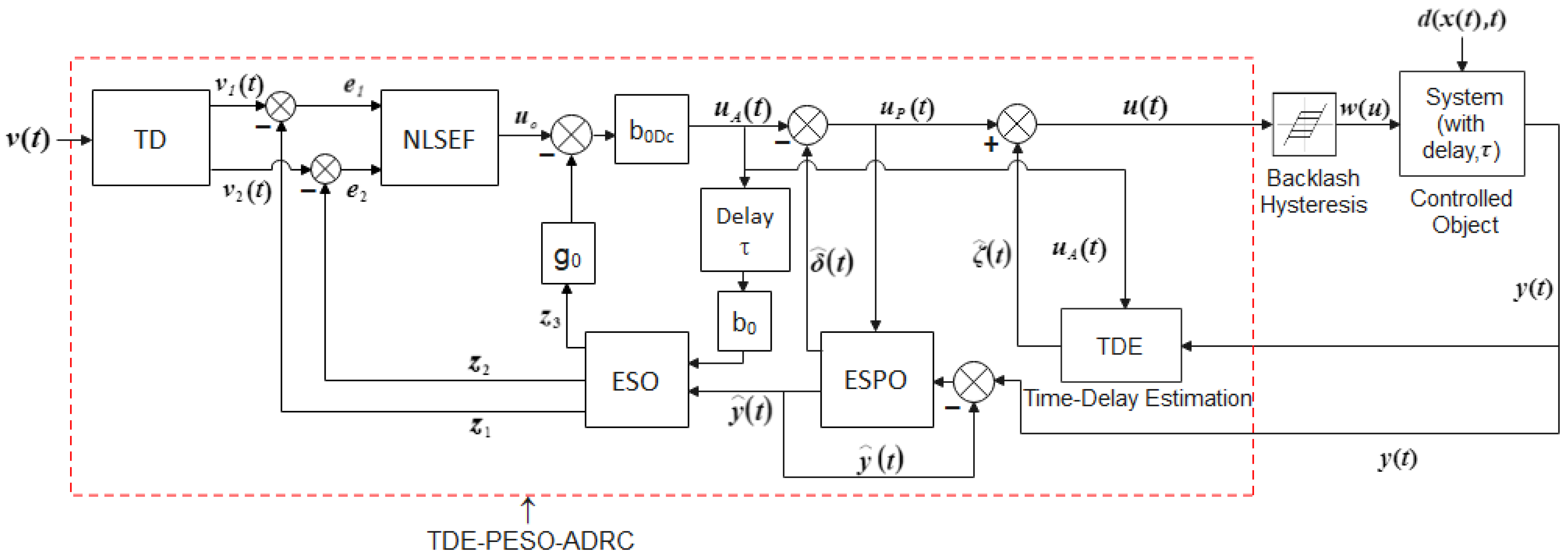
3. Modified ADRC Structures Using the TDE Mechanism

The TDE strategy is usually not used alone to provide estimation but integrated with other control techniques to obtain desired performance, such as steady-state error (SSE), robustness, disturbance rejection, overshoot, and rise time. Thus, in the following sections, it will be observed that the combination of the TDE scheme with the ADRC-based controllers (Figure 2 and Figure 3) benefits from the TDE mechanism’s simplicity and robustness. The signal in Equation (14) is considered the total disturbance acting on the system.

$$\delta \left(x\left(t\right),t\right)=d\left(x\left(t\right),t\right)+w\left(v_m\right)$$

(14)

where $\delta \left(x\left(t\right),t\right)$ corresponds to all the nonlinearities and input and output disturbances. $d\left(x\left(t\right),t\right)$ defines the different forms of impacts due to parameter perturbation and external disturbances applied to the system in Equation (3). $w\left(v_m\right)$ is the nonlinear backlash-like hysteresis shown in Equation (1).

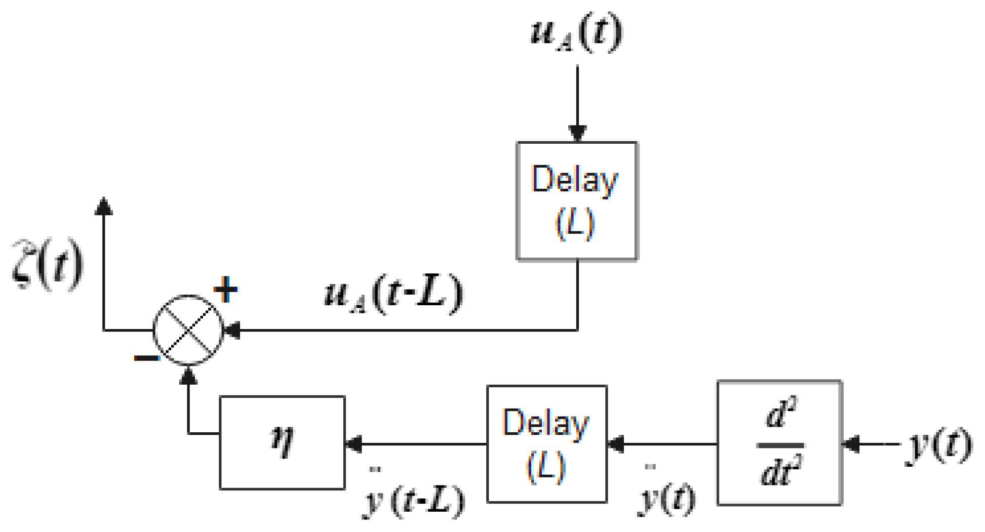
3.1. The TDE Mechanism

In this paper, the disturbance estimated by the TDE includes nonlinearity, backlash-like hysteresis, and other uncertainties acting on the controlled system in the presence of a time delay. For the controller’s simplicity and resilience to uncertainty, the TDE is given by Equations (15) and (16) and illustrated in Figure 4.

$$\widehat{\zeta }\left(t\right)=\zeta (t-L)$$

(15)

$$\zeta \left(t-L\right)=u_A\left(t-L\right)-\eta \ddot{y}(t-L)$$

(16)

where $\widehat{\zeta }\left(t\right)$ is the estimation of all uncertainties, and $(t-L)$ is the delayed term to estimate the unknown system dynamics. $\eta$ is a positive constant. Equation (16) shows that the TDE will provide a feasible model-free structure by estimating the current system dynamics based on system input and the dynamics of output only.

Further, from Equations (15) and (16), it is inferred that as the time delay $L$ (referred to as the sampling period in TDE) decreases, the estimate $\widehat{\zeta }\left(t\right)$ improves. Therefore, for the effective implementation of TDE, $L$ is chosen to be sufficiently small.

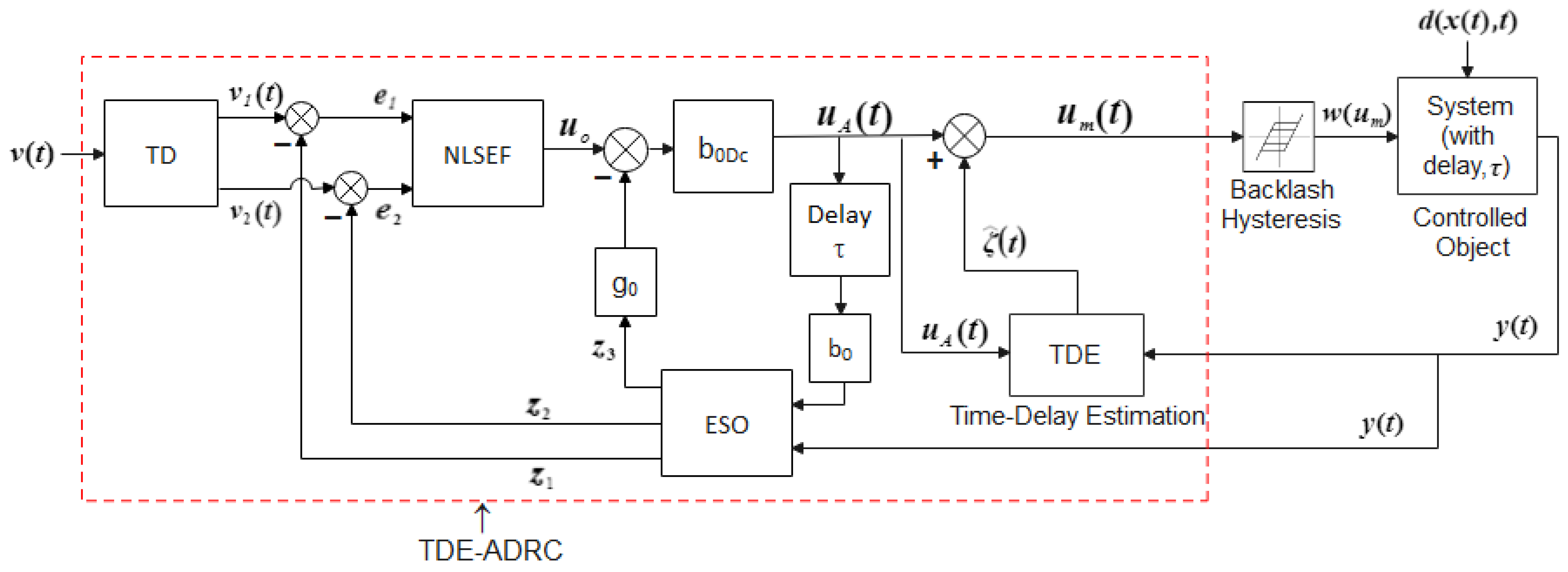
3.2. Integrate TDE in ADRC with Delayed Input

The modified controller design in Figure 5 combines the ADRC with time-delayed input (seen in Figure 2) with the TDE mechanism to obtain better controller performance by eradicating the effect of nonlinearities and uncertainties in the controlled object. This complete system is referred to as the TDE-ADRC. Here, the reference input signal fed to the TD is a step input signal $r\left(t\right)$, which produces transient profiles. The ESO subsystem performs disturbance estimation and compensation. Thus, the TD outputs supplied to the NLSEF provide a control law $u_0$ (in Equation (7)) to drastically lower the SSE of the signal obtained to zero in a limited time.

The system to be controlled by the modified ADRC methods is given by Equation (17):

$$\left\{\begin{array}{l}\dot{x}\left(t\right)=Ax\left(t\right)+B{u}_m\left(t\right)+\delta \left(x\left(t\right),t\right)\\ y\left(t\right)=C^{T}x\left(t-\tau \right)\end{array}\right.$$

(17)

where $x\left(t\right)$, $y\left(t\right),$ and $\tau$ are the state vector, output, and time delay of the system, respectively. The system’s state transition matrix, input matrix, and output matrix are represented by matrices $A$, $B$, and $C$, respectively. $\delta \left(x\left(t\right),t\right),$ which are the disturbances given in Equation (14). Further, the TDE block shown in Figure 5 provides the estimated disturbance $\widehat{\zeta }(t)$ given by Equations (15) and (16).

The resulting modified control law, $u_m\left(t\right),$ for the TDE-ADRC in Figure 5 is given by Equation (18):

$$\left\{\begin{array}{cc}\hfill u_m\left(t\right)& =u_A\left(t\right)+\widehat{\zeta }\left(t\right)\hfill \\ & =u_A\left(t\right)+\left(u_A\left(t-L\right)-\eta \ddot{y}\left(t-L\right)\right)\hfill \end{array}\right.$$

(18)

where $u_A\left(t\right)$ is obtained in Equation (10). $u_A\left(t-L\right)$ and $\ddot{y}\left(t-L\right)$ indicate the TDE operation involving the delayed input and the delayed dynamics of output, with a period $L$ and a positive constant $\eta$.

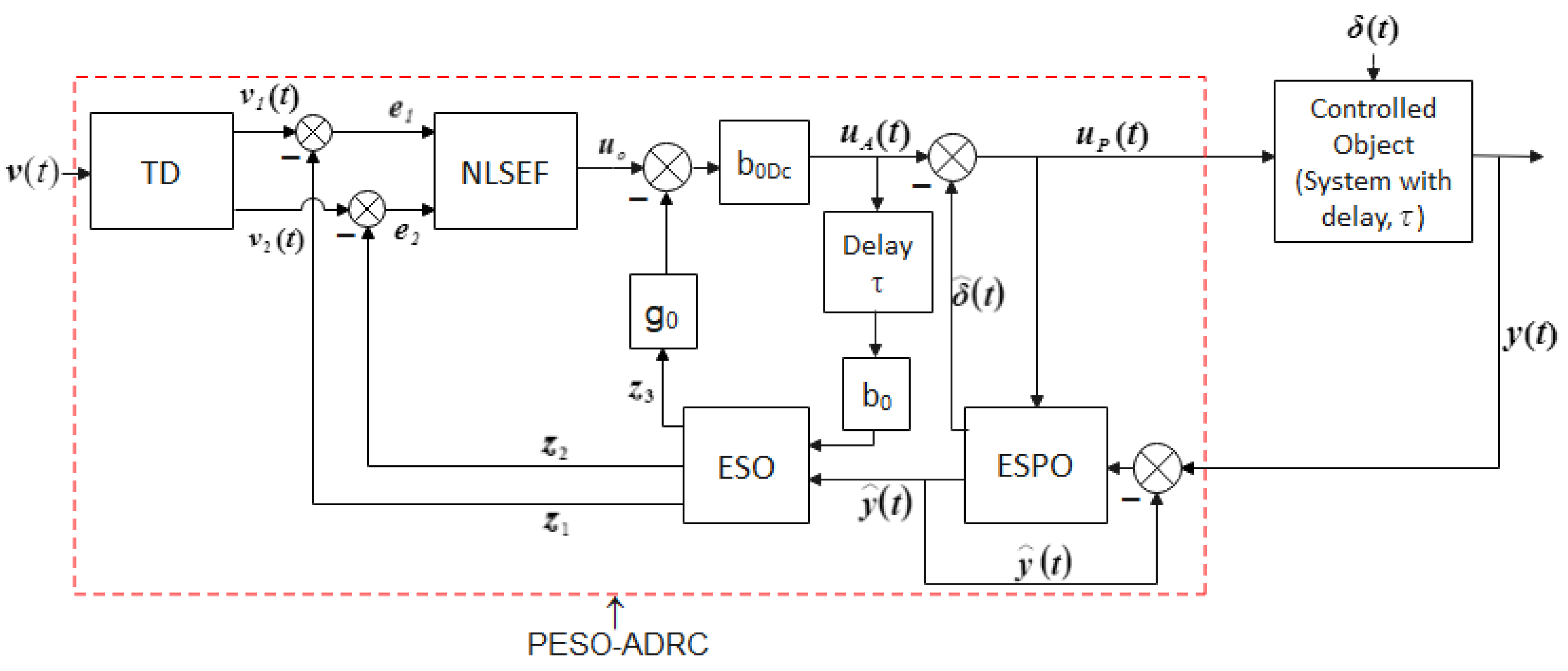
3.3. Integrate TDE into PESO-ADRC

Figure 6 gives a pictorial presentation of the incorporation of TDE with the PESO-ADRC (seen in Figure 3). The complete arrangement is referred to as TDE-PESO-ADRC in this paper, which is modeled by cascading the PESO-ADRC in Figure 3 with the TDE mechanism to enhance further the estimation and compensation of disturbances with backlash hysteresis nonlinearity added to the system. The system on which the uncertainties are acted upon is given in Equation (19).

$$\left\{\begin{array}{l}\dot{x}\left(t\right)=Ax\left(t\right)+Bu\left(t\right)+\delta \left(x\left(t\right),t\right)\\ y\left(t\right)=C^{T}x\left(t-\tau \right)\end{array}\right.$$

(19)

where $\delta \left(x\left(t\right),t\right)$ indicates the effects of both the disturbances and the nonlinearities present (Equation (14)). Subsequently, the modified control law $u\left(t\right)$ of the TDE-PESO-ADRC in Figure 6 is given by Equation (20):

$$\left\{\begin{array}{cc}\hfill u\left(t\right)& =u_P\left(t\right)+\widehat{\zeta }\left(t\right)\hfill \\ & ={(u}_A\left(t\right)-\widehat{\delta }\left(t\right))+\left(u_A\left(t-L\right)-\eta \ddot{y}\left(t-L\right)\right)\hfill \end{array}\right.$$

(20)

where $\widehat{\zeta }\left(t\right)$ is the TDE estimation given by Equations (15) and (16), and $u_P\left(t\right)$ is the control law for the PESO-ADRC in Equation (13).

4. Experimental Results, Analysis, and Discussions

In this section, to demonstrate the performance of the TDE mechanism in the modified ADRC methods in Figure 5 and Figure 6, a basic second-order time-delay system, represented by Equation (21), is employed in the experiments. Such a system is commonly used in industrial processes, wherein two first-order inertial systems are coupled with a time delay $\tau$ = 0.1 s. The state-space representation is shown in Equation (22).

$$G\left(s\right)={\displaystyle \frac{2}{s^2+3s+2}}{e}^{-\tau s}={\displaystyle \frac{1}{\left(0.5s+1\right)\left(s+1\right)}}{e}^{-\tau s}$$

(21)

$$\left\{\begin{array}{c}\dot{x}\left(t\right)=Ax\left(t\right)+Bu\\ y\left(t\right)=Cx\left(t-\tau \right)\end{array}\right.$$

(22)

where $A=\left[\begin{array}{cc}-3& 1\\ 2& 0\end{array}\right],B=\left[\begin{array}{c}0\\ 2\end{array}\right],C=\left[\begin{array}{cc}1& 0\end{array}\right]$.

For the system in Equation (21), the ADRC (Figure 2) parameters were optimized using the Genetic Algorithm (GA) under Optimization Tools in MATLAB Simulink software version R2020a [23]. The solver selection settings were set to automatic solver selection with a fixed step size of 0.001 s. The specific hardware system, that is, the laptop that was used to run the software and its simulations, has the following specifications: ASUS (Sonic Master), with a processor of the Intel(R) Core i7(TM)-7500U CPU @ 2.70 GHz 2.90 GHz, 8.00 GB of RAM, and a 64-bit operating system. Hence, the optimal parameter values obtained are $\left[c,h_1,r,g_0,b_0,b_{0DC}\right]$ = [0.7645, 1.0831, 56.0350, 0.3097, 3.1303, and 1.0314]. The ESO parameters are ${\beta }_{01}$ = 100, ${\beta }_{02}$ = 300, ${\beta }_{03}$ = 1000, and $h_{ESO}$ = 0.01. The unit-step signal is the reference input signal for all experiments.

Comparisons between the proposed TDE-ADRC and TDE-PESO-ADRC with the algorithms in [21,23] are conducted based on the integral of time-weighted absolute error—ITAE, and the transient response, including rise time, overshoot, and time to return to reference under hysteresis impact, to validate the proposed methods. Moreover, the proposed methods are also evaluated based on the ‘performance improvement (%)’ of an ITAE index value or a given transient characteristic (like rise time, settling time, and overshoot), denoted by $P_i$ in Equation (23):

$$P_i(\%)={\displaystyle \frac{P_0-P_1}{P_0}}\times 100\%$$

(23)

where $P_0$ is the transient characteristic value for ADRC with delayed input or the PESO-ADRC method without TDE, and $P_1$ is the transient characteristic value for ADRC with delayed input or the PESO-ADRC method with the integrated TDE mechanism.

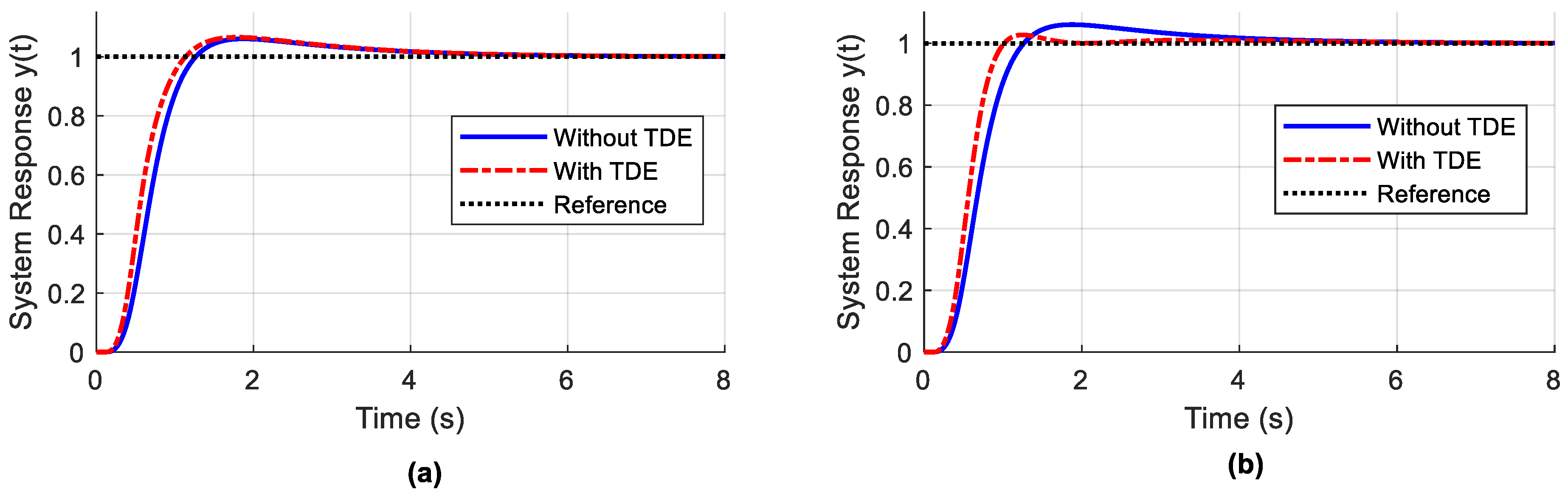
4.1. Effect of TDE on ADRC Methods without Backlash-Like Hysteresis or Disturbances

In this experiment, the proposed TDE-ADRC and TDE-PESO-ADRC are compared with their corresponding non-TDE mechanisms in [21,23] when no nonlinearity or disturbances are present in the controlled object Equation (21). In the TDE-ADRC, $\eta$ = 0.001 and $L$ = 0.001. In the TDE-PESO-ADRC, ${\omega }_e$ = 3, $\eta$ = 0.2, and $L$ = 0.002.

The corresponding system responses are illustrated in Figure 7a,b.

Table 1. Performance criteria of system response in the absence of hysteresis and disturbances.

Method	Performance Criteria	Without TDE	With TDE	${\mathit{P}}_{\mathit{i}}$ (%)
ADRC with delayed input	ITAE	0.5916	0.5480	7.3700
	Rise time (s)	0.6492	0.5806	10.5669
PESO-ADRC	ITAE	0.5916	0.2771	53.1609
	Rise time (s)	0.6492	0.4946	55.9300
	Settling time (s)	3.7300	1.4223	61.8686
	Overshoot (%)	5.9532	2.6234	55.9329

reports the performance index values for the step responses. From Figure 7, one finds that the system responses of the proposed methods were improved. In Figure 7a, with the TDE present, the controlled system responded faster, indicated by a shorter rise time (0.5806 s with TDE versus 0.6492 s without TDE), as shown in Table 1. However, the overshoot and settling time were not significantly improved. For the TDE-PESO-ADRC in Figure 7b and Table 1, the TDE, the ITAE, the rise time, the settling time, and the overshoot were improved. If comparing Figure 7a,b, one finds that PESO-ADRC also contributed to the performance.

To provide more details, in TDE-PESO-ADRC, the overshoot decreases by 55.9% compared to the case without the TDE mechanism. Moreover, the ITAE values in Table 1 are smaller when TDE is integrated. Hence, the performance improvement (%) results in Table 1 illustrate the significance of integrating TDE with ADRC methods for estimating and compensating unknown system dynamics.

4.2. Effect of TDE on ADRC Methods under Hysteresis

In this experiment, the controlled object in Equation (21) is subjected to a Duhem backlash-like model representing an active hysteresis that significantly influences the system response. For the sake of even comparison in the following experiments, the hysteresis model parameters selected in Equation (1) are γ = 0.1, α = 1.16, and β = 0.35. The TDE parameters for the TDE-ADRC are $\eta$ = 0.001 and $L$ = 0.001, whereas the TDE-PESO-ADRC are ${\omega }_e$ = 4, $\eta$ = 0.001, and $L$ = 0.001. The total uncertainty given by Equation (14) is $\delta \left(x\left(t\right),t\right)=w\left(v_m\right)$, where $w\left(v_m\right)$ defines the hysteresis output in Equation (1).

Figure 8a,b depict the relevant results that show how TDE performs in combating the nonlinear backlash hysteresis imposed on the controlled object. The unit-step response performance is shown in

Table 2. Performance criteria of system response in the case of hysteresis present.

Method	Performance Criteria	Without TDE	With TDE	${\mathit{P}}_{\mathit{i}}$ (%)
ADRC with delayed input	ITAE	2.3790	0.4152	82.5473
	Rise time (s)	0.6525	0.4208	31.7886
	Settling time (s)	6.2432	2.4114	61.3756
	Overshoot (%)	29.7770	20.3113	31.7886
PESO-ADRC	ITAE	5.3570	1.0130	81.0901
	Rise time (s)	0.6715	0.4032	52.0444
	Settling time (s)	10.9744	4.8639	55.6796
	Overshoot (%)	43.3960	20.8108	52.0444

, where the ITAE values are 0.4152 and 1.0130 for the proposed TDE-ADRC and TDE-PESO-ADRC, respectively, which are much smaller than the original methods without TDE integrated. Figure 8 shows that the systems responded faster when TDE was present, with a smaller rise time, as shown in Table 2. Figure 8a,b illustrate that TDE also improved the settling time. Under the hysteresis effect with TDE present, it is shown in Table 2 that the overshoots were reduced by 31.8% and 52% for the ADRC with delayed input and the PESO-ADRC methods, respectively. Moreover, Figure 8b shows that the TDE reduced the oscillatory behavior of the system response.

Hence, the experimental results on performance improvement (%) in Table 2 illustrate that the proposed methods effectively estimate, control, and compensate for the nonlinear hysteresis phenomenon with improved robustness, quick recovery, and stability in system response.

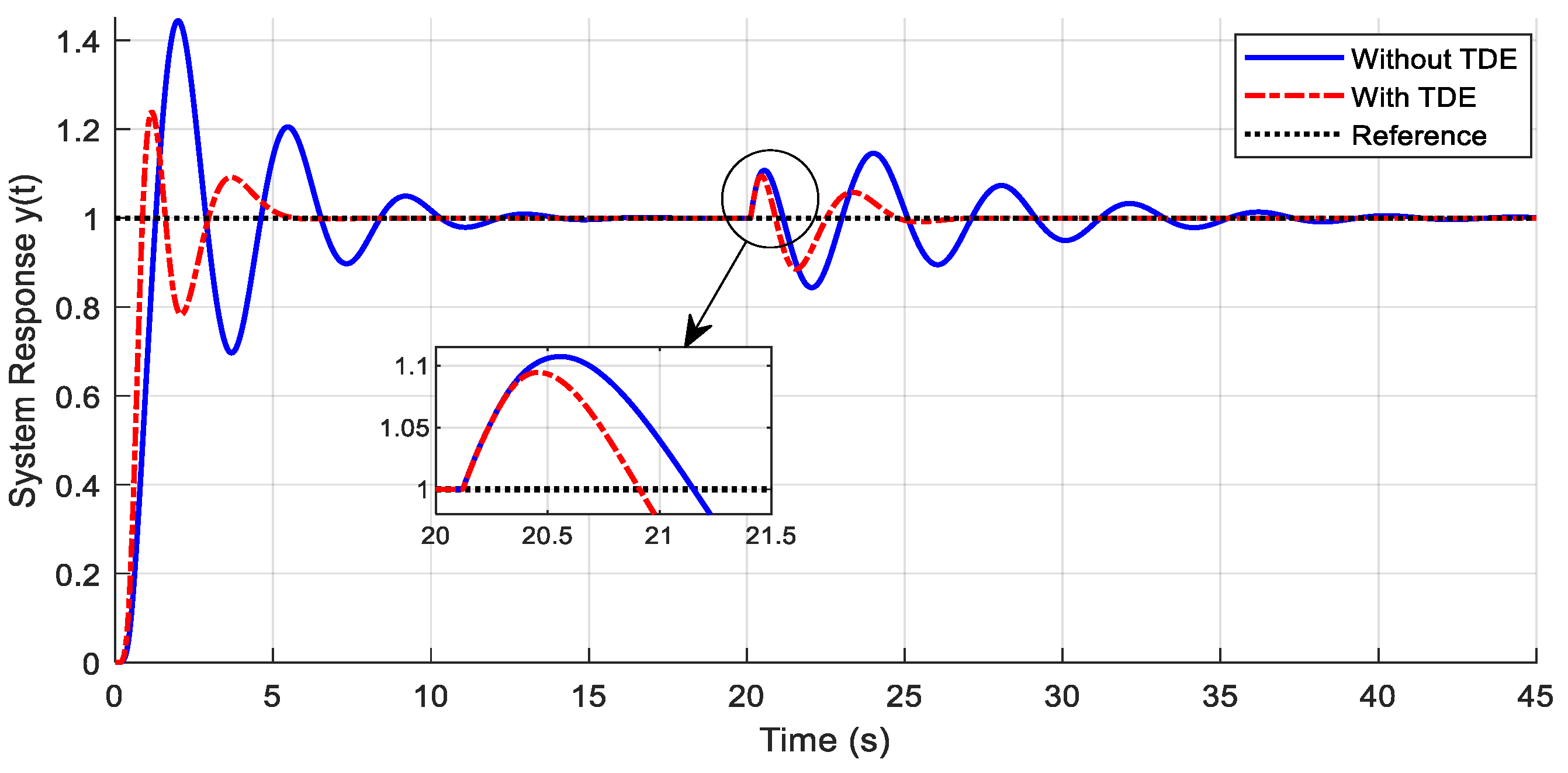
4.3. Effect of TDE on ADRC Methods under Both Hysteresis and Parameter Perturbation

In this experiment, along with the backlash-like hysteresis acting at the 20th second, a system parameter perturbation of 20% is applied when both the system time constants and the time delay are increased by 20%. Then, the TDE is used to overcome parameter perturbation and nonlinearity compensation. Hence, the respective perturbed system $\tilde{G}\left(s\right)$ is represented using the transfer function and state-space representation given by Equations (24) and (25), respectively.

$$\tilde{G}\left(s\right)={\displaystyle \frac{1.3889}{s^2+2.5s+1.3889}}{e}^{-0.12s}$$

(24)

$$\left\{\begin{array}{c}\dot{\tilde{x}}=\tilde{A}\tilde{x}+\tilde{B}u\\ \tilde{y}=\tilde{C}\tilde{x}\left(t-\tilde{\tau }\right)\end{array}\right.$$

(25)

where $\tilde{A}=\left[\begin{array}{cc}-2.5& 1\\ -1.3889& 0\end{array}\right],\tilde{B}=\left[\begin{array}{c}0\\ 1.3889\end{array}\right],\tilde{C}=\left[\begin{array}{cc}1& 0\end{array}\right]$, $\tilde{\tau }$ = 0.12 s. In this experiment as well, the hysteresis model parameters in Equation (1) are selected as γ = 0.1, α = 1.16, and β = 0.35. The TDE parameters for the TDE-ADRC and the TDE-PESO-ADRC are as follows: $\eta$ = 0.001 and $L$ = 0.001. For the TDE-PESO-ADRC, ${\omega }_e$ = 4. The total uncertainty given by Equation (14) is $\delta \left(x\left(t\right),t\right)=w\left(v_m\right)+d\left(x\left(t\right),t\right)$, where $w\left(v_m\right)$ is the hysteresis output and $d\left(x\left(t\right),t\right)$ refers to impacts due to the system parameter perturbation.

Figure 9 and Figure 10 demonstrate the responses of the ADRC methods with TDE under the effects of hysteresis and system parameter perturbation. The performance index measures are also listed in

Table 3. Performance criteria of system response for the case of hysteresis and parameter perturbation present.

Method	Performance Criteria	Without TDE	With TDE	${\mathit{P}}_{\mathit{i}}$ (%)
ADRC with delayed input	ITAE	19.9800	5.7420	71.2613
	Rise time (s)	0.6725	0.4132	24.9301
	Settling time (s)	25.8333	22.9382	11.2069
	Overshoot (%) [from 0 to 3 s]	30.3688	22.7978	24.9302
	Overshoot (%) [from 20 to 22 s]	8.5700	7.2900	14.9358
PESO-ADRC	ITAE	27.9900	6.7860	75.7556
	Rise time (s)	0.6931	0.4010	46.1113
	Settling time (s)	34.4842	24.3004	29.5318
	Overshoot (%) [from 0 to 3 s]	44.2609	23.8516	46.1114
	Overshoot (%) [from 20 to 22 s]	10.7500	9.4600	12.0000

.

As shown in Figure 9, with the help of TDE, in the transient response, the TDE-ADRC-controlled system output rose faster, and the overshoot was smaller (around 22.8% with TDE versus 30.4% without TDE). From Table 3, one gets that the overshoot at the initial transient response is reduced by almost 25% compared to controller operation without the TDE. Then, under the influence of parameter perturbation starting at 20 s, the TDE-ADRC experienced less overshoot and recovered the final value faster. Then, under the influence of parameter perturbation starting at 20 s, the TDE-ADRC experienced less overshoot, and the ITAE values were smaller. Moreover, the TDE-ADRC method showed an improved settling time and recovered the final value faster.

In Figure 10, the overshoot and the settling time in the initial transient response were significantly reduced by the TDE mechanism. Moreover, the TDE-PESO-ADRC method is less susceptible to oscillations. In Table 3, the $P_i$(%) relating to overshoot at the initial transient response (from 0 to 3 s) is 46.1%, whereas under the impact of parameter perturbation (from 20 to 22 s), it is 12%. Hence, the TDE-PESO-ADRC illustrated higher robustness and decent resilience to hysteresis and parameter perturbation in the controlled object.

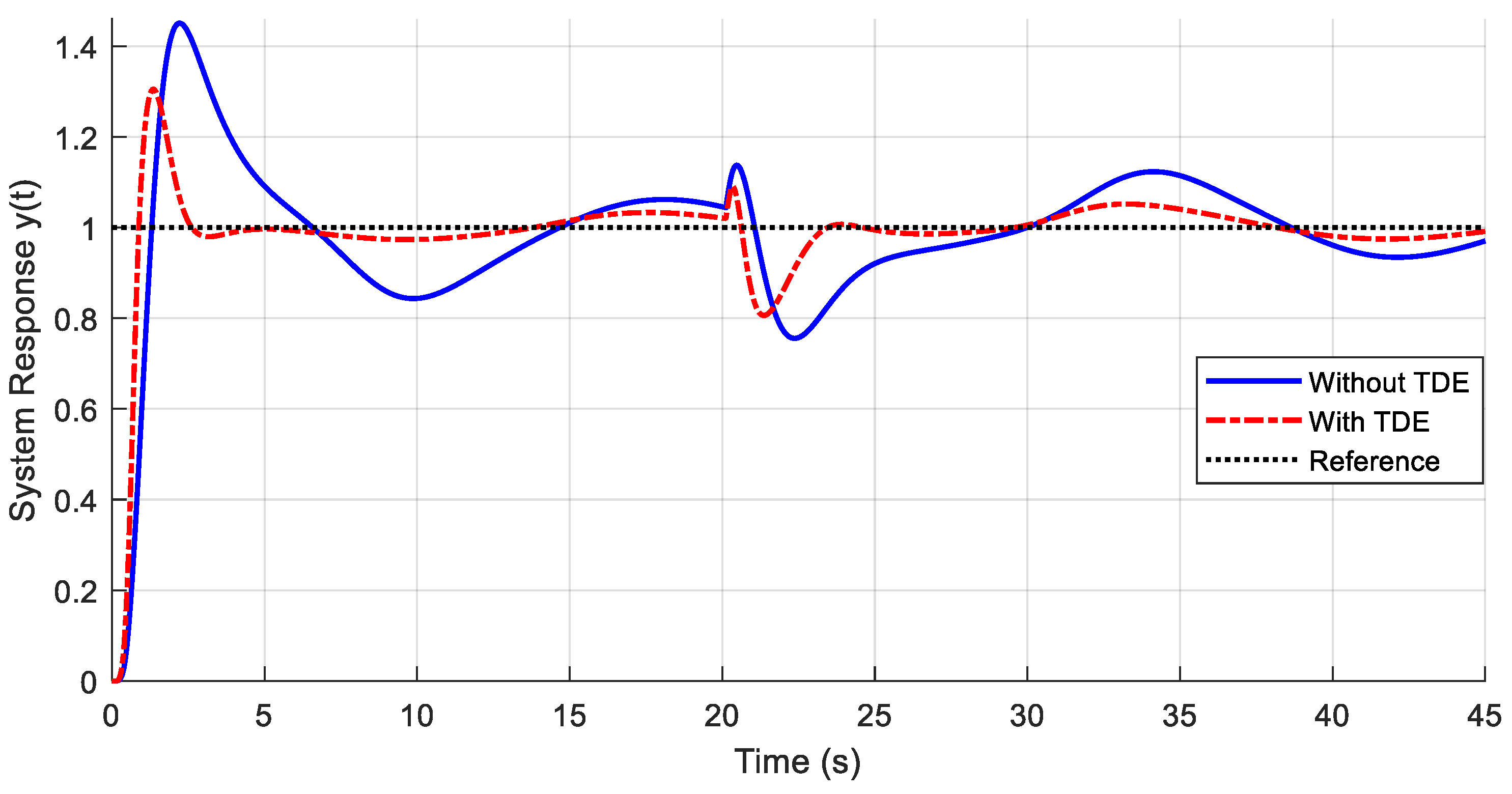
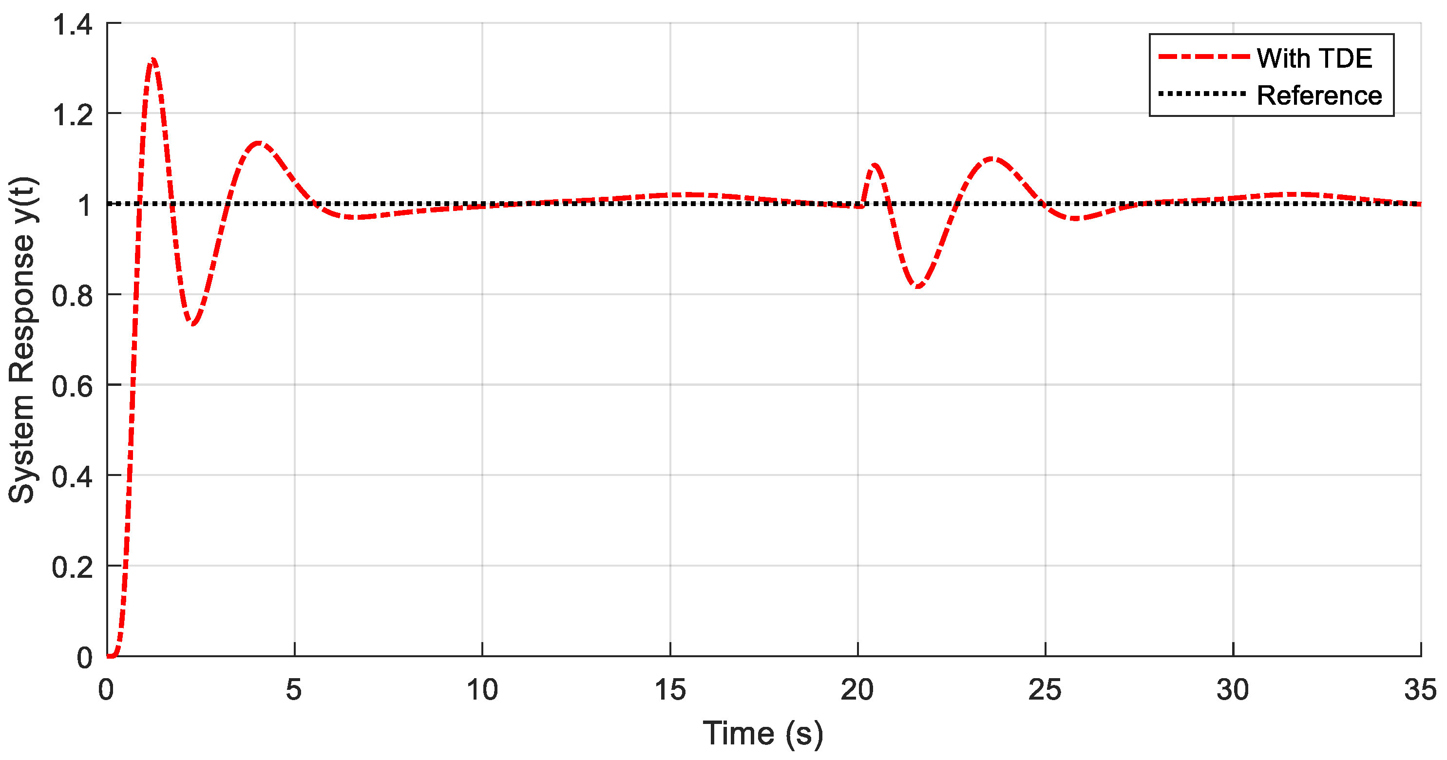
4.4. Effect of TDE on ADRC Methods under Hysteresis, Parameter Perturbation, and External Disturbance

This experiment continues from the one in the previous subsection, wherein hysteresis and a system parameter perturbation of 20% incrementation are applied at 20 s. Additionally, an external disturbance is applied as an input disturbance to the controlled object. Therefore, the total applied uncertainties and disturbances are given by $\delta \left(x\left(t\right),t\right)=d\left(x\left(t\right),t\right)+w\left(v_m\right)$, wherein the hysteresis effect is indicated by $w\left(v_m\right)$. In this experiment, $d\left(x\left(t\right),t\right)$ is a combination of the effects of parameter perturbation and external disturbance ($d_1\left(x\left(t\right),t\right)$ given in Equation (26)).

$$d_1\left(x\left(t\right),t\right)=-0.2e^{{\mathrm{c}\mathrm{o}\mathrm{s}x}_2}+0.1u+0.2\mathrm{s}\mathrm{i}\mathrm{g}\mathrm{n}(\sin {\displaystyle \frac{\pi }{8t}})$$

(26)

The parameters for TDE, the hysteresis model, and the PESO-ADRC observer bandwidth are the same as defined in the previous section. Figure 11 and Figure 12 illustrate the responses of the TDE-ADRC and TDE-PESO-ADRC under the effects of hysteresis, system parameter perturbation, and external disturbance, with their performance index measures in

Table 4. Performance criteria of system response for the case of hysteresis, parameter perturbation, and external disturbance present.

Method	Performance Criteria	Without TDE	With TDE	${\mathit{P}}_{\mathit{i}}$ (%)
ADRC with delayed input	ITAE	70.6600	26.8400	62.0153
	Rise time (s)	0.6732	0.4047	39.8841
	Overshoot (%) [from 0 to 3 s]	49.5175	31.6211	36.0000
	Overshoot (%) [from 20 to 22 s]	13.5500	9.1000	32.8413
PESO-ADRC	ITAE	Unstable	15.9200	-
	Rise time (s)	Unstable	0.4017	-
	Overshoot (%) [from 0 to 3 s]	Unstable	32.0155	-
	Overshoot (%) [from 20 to 22 s]	Unstable	8.5000	-

.

Figure 11 shows that with the TDE present, the controlled system showed a smaller rise time, as shown in Table 4. Further, in the initial transient response, the overshoot was reduced by 36% ($P_i$%) due to the TDE mechanism in the TDE-ADRC. Further, from 20 to 22 s, the overshoot was reduced by 32.8%. Moreover, after the introduction of the system input disturbance (Equation (26)), one finds that the amplitude of the oscillatory response was reduced by around 28% using the TDE mechanism (between 30 s and 40 s). Due to the oscillatory nature of the added external disturbance, the settling time is not recorded in Table 4.

After introducing external disturbance with the present nonlinear hysteresis and parameter perturbation, the PESO-ADRC without the TDE mechanism is unstable, thus could not be plotted in Figure 12. Thus, performance improvement (%) could not be calculated for PESO-ADRC in Table 4. However, by adding the TDE mechanism in this scenario, the TDE-PESO-ADRC overcame this unstable behavior and produced a decent response curve showing good resilience to system uncertainties (Figure 12 and Table 4). Hence, this highlights the importance of the TDE mechanism in estimating and compensating for the total nonlinearities in time-delay system control.

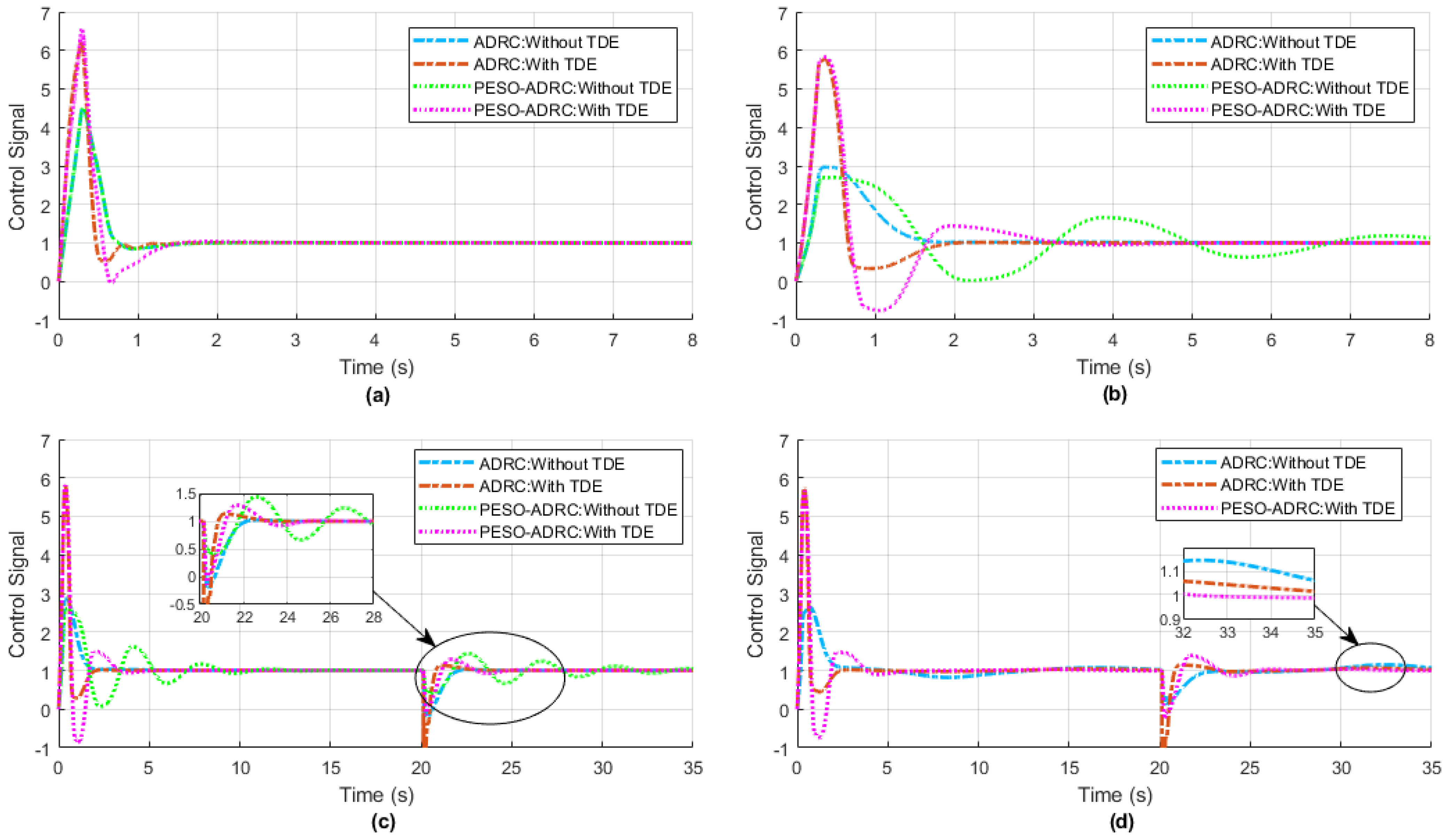
4.5. Control Signal for Different Scenarios

This section demonstrates the simulation results of the control signal fed to the controlled object under consideration for both the ADRC with delayed input method and the PESO-ADRC method for the cases with and without the TDE mechanism, respectively. Figure 13a presents the control signal performance for the experiment performed in Section 4.1 of this study, that is, under the effects of the absence and presence of TDE alone on both ADRC methods without backlash hysteresis or other uncertainties present. Further, Figure 13b illustrates the control signal for the case of hysteresis present in the experiment performed in Section 4.2. Here, in the case of TDE present, the control signal is less oscillatory and reaches a steady state earlier than in the case without TDE.

Furthermore, Figure 13c provides the control signal plots of the experiment conducted under Section 4.3, with both hysteresis and parameter perturbation present. It is visible from the zoomed-in plot of Figure 13c when the parameter perturbation occurs at 20 s; the TDE-PESO-ADRC suppresses the shift from the reference value to a decent extent by limiting the oscillations sustained due to the application of parameter perturbation. Similarly, due to the hysteresis present, the oscillatory response in the initial phase of the plot is greatly limited by the integrated TDE mechanism. Moreover, Figure 13d depicts the control signal behavior for hysteresis, parameter perturbation, and an added external disturbance acting on the controlled object (Section 4.4). It can be interpreted from the control signal responses that the proposed TDE-ADRC methods showed fair recovery under the effect of nonlinearity and uncertainties, along with attaining a zero SSE for the TDE-PESO-ADRC method, as seen in the zoomed-in plot of Figure 13d. Due to the unstable response of the PESO-ADRC method in the absence of TDE, the response is not plotted in Figure 13d.

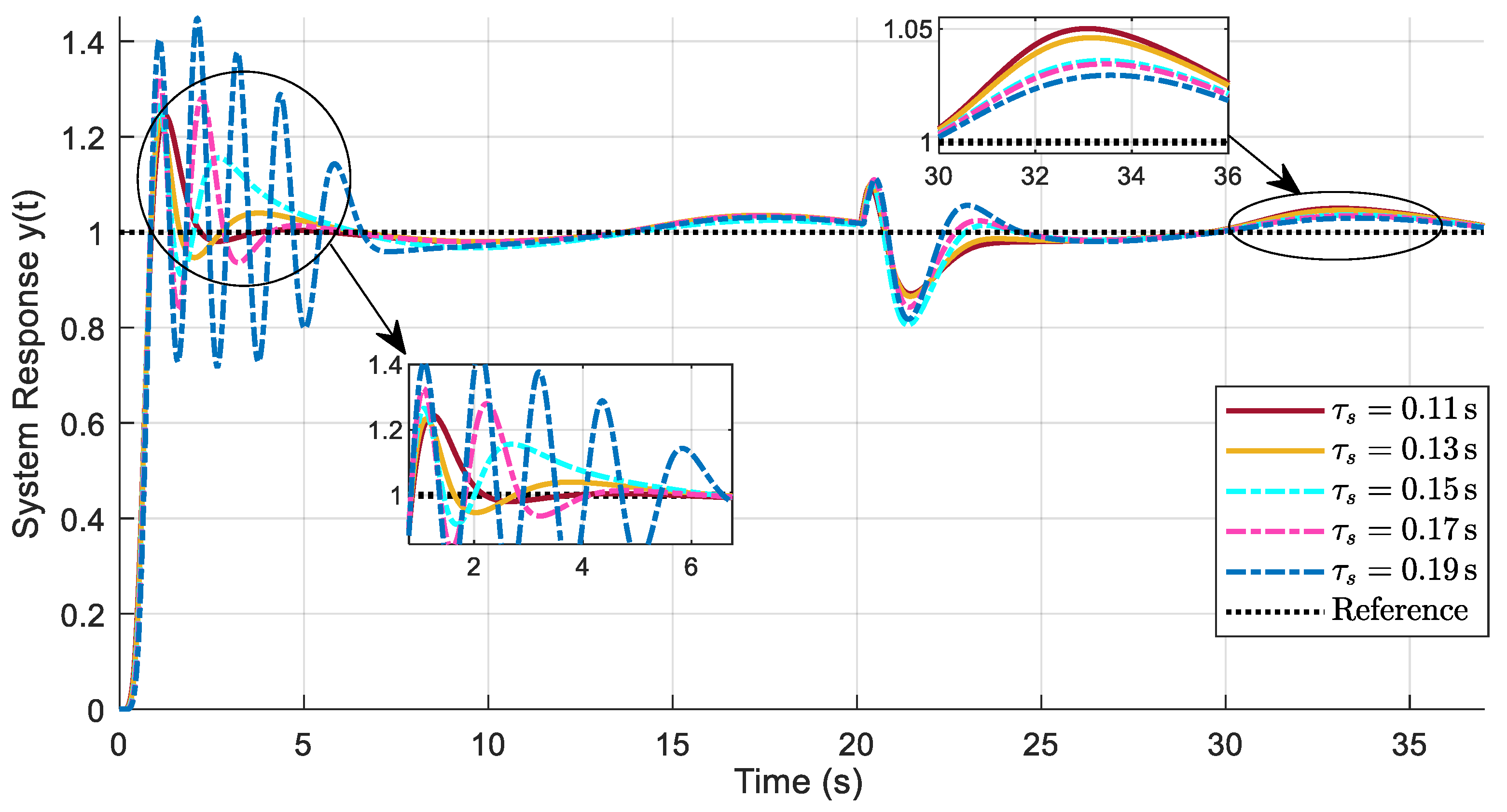
4.6. Effect of Change in System Time Delay on the Proposed TDE-ADRC Methods

This section measures the robustness of the proposed TDE-ADRC methods for different system delay values in the presence of hysteresis, parameter perturbations, and external disturbances acting on the system. In this experimental test, the delay ${\tau }_s$ corresponds to the system delay of the controlled object (seen in Figure 5 and Figure 6). The parameters for the TDE mechanism, the hysteresis model, 20% system parameter perturbation, and the external (input) disturbance applied remain the same from the experiment performed in Section 4.4. When testing the robustness of the proposed TDE-ADRC mechanisms, the delay value contained in the ADRC (Figure 5 and Figure 6 at the input path to ESO) and in the ESPO (Figure 6) stays the same, 0.1 s, and this delay is termed delay design in this experiment. Whereas in this test for testing the robustness, ${\tau }_s$ is varied over different known delay values. (In the previous experiments, ${\tau }_s$ = 0.1 s).

Figure 14 and Figure 15 demonstrate the effect of changes in system delay on the proposed TDE-ADRC and TDE-PESO-ADRC methods, respectively. In Figure 14, ${\tau }_s$ = 0.11 s, 0.13 s, 0.15 s, 0.17 s, and 0.19 s. Thus, the system delay was increased by 10%, 30%, 50%, 70%, and 90% from the 0.1 s system delay, respectively. Whereas in Figure 15, ${\tau }_s$ = 0.11 s, 0.13 s, 0.15 s, and 0.17 s, indicating an increase in 10%, 30%, 50%, and 70% from a 0.1 s system delay. Therefore, Figure 14 and Figure 15 show that for higher system delay, the proposed TDE-ADRC method response curves were oscillatory but did achieve compensation for nonlinearity and disturbances, hence showing robust and stable behavior under different delay scenarios.

Table 5. Performance metrics of the TDE-ADRC method’s response to different system time delays.

TDE-ADRC	Rise Time (s)	Response Time (s)	Overshoot (%)	ITAE
${\tau }_s$ = 0.11 s	0.4037	35.3057	22.8240	20.1500
${\tau }_s$ = 0.13 s	0.3769	35.2035	21.7502	19.3200
${\tau }_s$ = 0.15 s	0.3552	34.7406	25.1789	18.6900
${\tau }_s$ = 0.17 s	0.3392	34.6135	31.1730	17.3100
${\tau }_s$ = 0.19 s	0.3270	28.6165	43.4998	20.5000

and

Table 6. Performance metrics of the TDE-PESO-ADRC method’s response to different system time delays.

TDE-PESO-ADRC	Rise Time (s)	Response Time (s)	Overshoot (%)	ITAE
${\tau }_s$ = 0.11 s	0.3893	33.1176	31.4353	15.0600
${\tau }_s$ = 0.13 s	0.3728	33.0609	36.6789	15.6000
${\tau }_s$ = 0.15 s	0.3605	32.9865	43.7253	18.2300
${\tau }_s$ = 0.17 s	0.3516	32.8235	58.4140	33.1700

tabulate the performance metrics of the system response curves, such as the rise time, response time, overshoot, and ITAE performance index value. In Table 5 and Table 6, the response time indicates the instant the system could achieve a steady state after backlash like hysteresis, nonlinearity, and disturbance compensation.

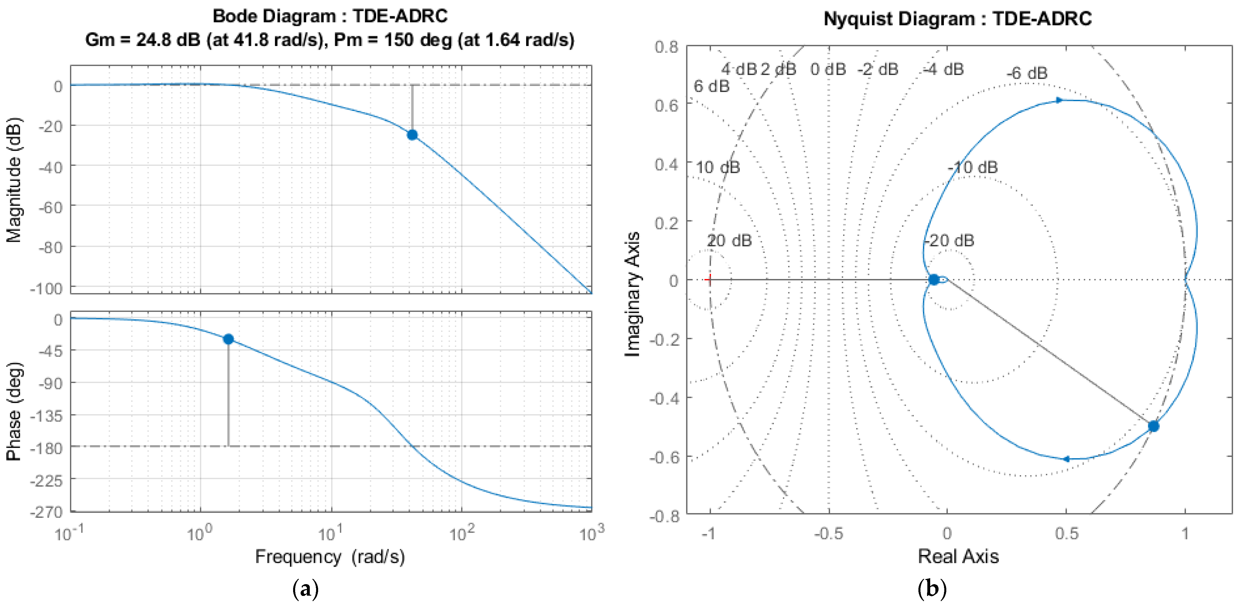
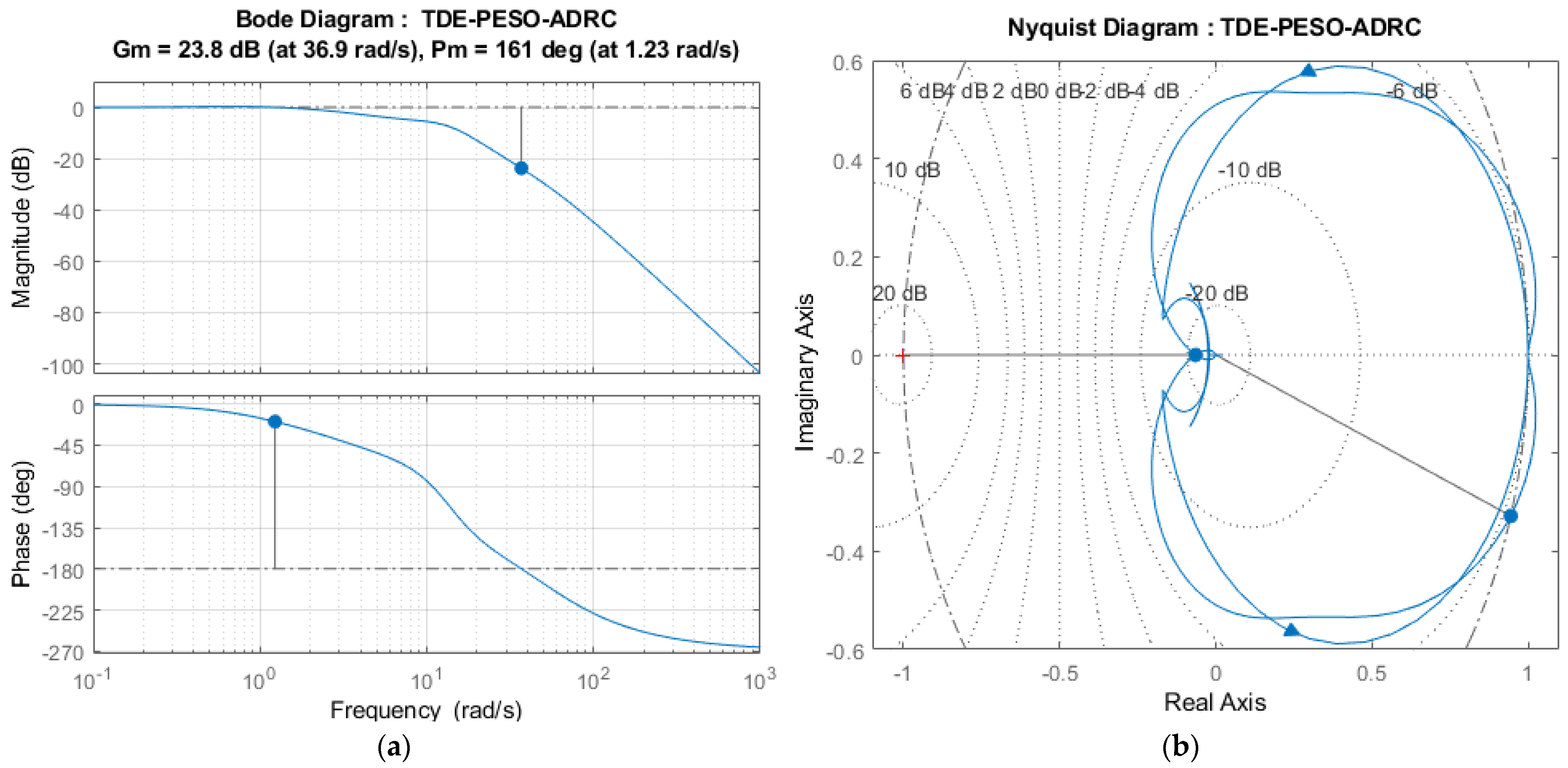
4.7. Stability Analysis of the Proposed TDE-ADRC Methods

This section analyzes the stability analysis of the proposed TDE-ADRC and the TDE-PESO-ADRC methods using frequency domain analysis techniques such as the open-loop Bode diagram and the Nyquist criterion. The former consists of the magnitude plot that provides the gain margin (Gm) in decibels (dB) and the phase plot that provides the phase margin (Pm) in degrees. The latter is effectively used in the case of non-minimum phase analysis. Figure 16 and Figure 17 indicate the frequency responses of the linearized system for the proposed TDE-ADRC and TDE-PESO-ADRC controller designs, respectively. Like the previous experiments, the system (controlled object) given by Equation (21) is controlled by the proposed TDE-ADRC and TDE-PESO-ADRC methods to perform the stability analysis.

In the open-loop Bode plot for the TDE-ADRC method given by Figure 16a, the Gm obtained at a phase crossover frequency of 41.8 rad/s is 24.8 dB, whereas the Pm is 150° at a gain crossover frequency of 1.64 rad/s. Since both Gm and Pm are positive, the system is closed-loop stable. Further, a delay margin of 1.6 s is obtained from the phase plot of Figure 16a. Hence, this indicates that the proposed TDE-ADRC system will begin to incur instability when the time delay is approximately greater than the delay margin. Stability is further verified in Figure 16a by the phase crossover frequency (41.8 rad/s) exceeding the gain crossover frequency (1.64 rad/s). Furthermore, Figure 16b shows that the critical point (−1, j0) is not encircled; thus, this observation agrees with the Nyquist criterion and validates the system’s stability.

Figure 17 provides the stability analysis of the TDE-PESO-ADRC method proposed in this study. From the open-loop Bode plot in Figure 17a, the Gm is 23.8 dB at a phase crossover frequency of 36.9 rad/s, and the Pm is 161° at a gain crossover frequency of 1.23 rad/s. Hence, the overall system is analyzed as being closed-loop stable. Moreover, the delay margin obtained from the phase plot is 2.28 s, indicating that the system is stable for delays under 2.28 s. The stability is further substantiated by obtaining a phase crossover frequency of 36.9 rad/s, greater than the gain crossover frequency of 1.23 rad/s. Furthermore, the stability of the proposed TDE-PESO-ADRC method is further analyzed using the Nyquist diagram, which captures the effects of right-hand pole zeros and their impact on the system’s stability and behavior. As illustrated in Figure 17b, no encirclement of the critical point (−1, j0) was obtained, proving the system’s stability per the Nyquist criterion.

5. Conclusions

This paper proved that the TDE is crucial for enhancing disturbance rejection operations in ADRC-controlled time-delay systems. After integrating the TDE with the ADRC with delayed input and PESO-ADRC methods, we obtained the new control laws. The TDE showed stronger capacity to conquer the nonlinearity-related challenges in the ADRC-controlled systems, which forms the main contribution of this paper.

The experimental results compared and analyzed the impacts of TDE on ADRC with delayed input and PESO-ADRC in the presence of different uncertainties in the controlled time-delay systems. The results indicated that utilizing the TDE for both the PESO-ADRC and ADRC with delayed input systems improved the response significantly under backlash-like hysteresis, system uncertainties like parameter perturbation, external disturbance, fixed time delay, and different system delays. The proposed methods exhibited stability, robustness, and transient steady-state response by diminishing the oscillations under the impact of nonlinearities, followed by their speedy estimation and compensation compared to their non-TDE counterparts.

Overall, the paper provided a novel perspective on ADRC’s disturbance estimation mechanism through a TDE interpretation, offering valuable insights for engineers and researchers working on ADRC strategies, particularly in future directions involving human-machine interface systems. Further research suggests enhancing the TDE mechanism in applications involving systems dealing with different forms of nonlinearities, uncertainties, noise, and varying time delay values to implement on real-world platforms. These challenges can be addressed by introducing an adaptive TDE mechanism, followed by its stability-proof analysis, thus forming part of further continuing study.

References

1. Han, J. From PID to Active Disturbance Rejection Control. IEEE Trans. Ind. Electron. 2009, 56, 900–906. [Google Scholar] [CrossRef]
2. Han, J.Q. Auto Disturbance Rejection Controller and It’s Applications. Control Decis. 1998, 13, 19–23. [Google Scholar]
3. Nahri, S.N.F.; Du, S.; van Wyk, B.J.; Nyasulu, T.D. Mitigating the Time Delay and Parameter Perturbation by a Predictive Extended State Observer-based Active Disturbance Rejection Control. In Proceedings of the Towards Autonomous Robotic Systems: 25th Annual Conference, TAROS 2024, Springer Lecture Notes in Artificial Intelligence (LNAI) Series, London, UK, 21–23 August 2024. in press. [Google Scholar]
4. Shamsuzzoha, M.; Raja, G.L. Disturbance Rejection Control; IntechOpen: London, UK, 2023. [Google Scholar] [CrossRef]
5. Xu, L.; Zhuo, S.; Liu, J.; Jin, S.; Huangfu, Y.; Gao, F. Advancement of active disturbance rejection control and its applications in power electronics. IEEE Trans. Ind. Appl. 2023, 60, 1680–1694. [Google Scholar] [CrossRef]
6. Zheng, Q.; Gao, Z. Active disturbance rejection control: Some recent experimental and industrial case studies. Control Theory Technol. 2018, 16, 301–313. [Google Scholar] [CrossRef]
7. Fareh, R.; Khadraoui, S.; Abdallah, M.Y.; Baziyad, M.; Bettayeb, M. Active disturbance rejection control for robotic systems: A review. Mechatronics 2021, 80, 102671. [Google Scholar] [CrossRef]
8. Wu, Z.; Gao, Z.; Li, D.; Chen, Y.; Liu, Y. On transitioning from PID to ADRC in thermal power plants. Control Theory Technol. 2021, 19, 3–18. [Google Scholar]
9. Hezzi, A.; Elbouchikhi, E.; Bouzid, A.; Ben Elghali, S.; Zerrougui, M.; Benbouzid, M. Active Disturbance Rejection Control for Distributed Energy Resources in Microgrids. Machines 2024, 12, 67. [Google Scholar] [CrossRef]
10. Nahri, S.N.F.; Du, S.; van Wyk, B.J. Active Disturbance Rejection Control Design for a Haptic Machine Interface Platform. Adv. Sci. Technol. Eng. Syst. J. 2021, 6, 898–911. [Google Scholar]
11. Nahri, S.N.F.; Du, S.; Van Wyk, B.J. A Review on Haptic Bilateral Teleoperation Systems. J. Intell. Robot. Syst. 2022, 104, 13. [Google Scholar] [CrossRef]
12. Goforth, F.J.; Gao, Z. An active disturbance rejection control solution for hysteresis compensation. In Proceedings of the 2008 American Control Conference, Seattle, WA, USA, 11–13 June 2008; pp. 2202–2208. [Google Scholar]
13. Liu, W.; Cheng, L.; Hou, Z.-G.; Tan, M. An active disturbance rejection controller with hysteresis compensation for piezoelectric actuators. In Proceedings of the 2016 12th World Congress on Intelligent Control and Automation (WCICA), Guilin, China, 12–15 June 2016; pp. 2148–2153. [Google Scholar]
14. Liu, W.; Zhao, T. An active disturbance rejection control for hysteresis compensation based on neural networks adaptive control. ISA Trans. 2021, 109, 81–88. [Google Scholar] [CrossRef]
15. Liu, W.; Zhao, T.; Wu, Z.; Huang, W. Linear active disturbance rejection control for hysteresis compensation based on backpropagation neural networks adaptive control. Trans. Inst. Meas. Control 2021, 43, 915–924. [Google Scholar] [CrossRef]
16. Du, S.; van Wyk, B.; Nahri, N.; Tu, C. Auto Disturbance Rejection Control Based on A Neural Network Predictive State Observer. In Proceedings of the 2023 15th International Conference on Intelligent Human-Machine Systems and Cybernetics (IHMSC), Hangzhou, China, 26–27 August 2023; pp. 233–236. [Google Scholar]
17. Chen, S.; Xue, W.; Zhong, S.; Huang, Y. On comparison of modified ADRCs for nonlinear uncertain systems with time delay. Sci. China Inf. Sci. 2018, 61, 70223. [Google Scholar] [CrossRef]
18. Ran, M.; Wang, Q.; Dong, C.; Xie, L. Active disturbance rejection control for uncertain time-delay nonlinear systems. Automatica 2020, 112, 108692. [Google Scholar] [CrossRef]
19. Xue, W.; Liu, P.; Chen, S.; Huang, Y. On extended state predictor observer based active disturbance rejection control for uncertain systems with sensor delay. In Proceedings of the 2016 16th International Conference on Control, Automation and Systems (ICCAS), Gyeongju, Republic of Korea, 16–19 October 2016; pp. 1267–1271. [Google Scholar]
20. Tan, W.; Fu, C. Analysis of active disturbance rejection control for processes with time delay. In Proceedings of the 2015 American control conference (ACC), Chicago, IL, USA, 1–3 July 2015; pp. 3962–3967. [Google Scholar]
21. Zhao, S.; Gao, Z. Modified active disturbance rejection control for time-delay systems. ISA Trans. 2014, 53, 882–888. [Google Scholar] [CrossRef]
22. Fu, C.; Tan, W. Linear active disturbance rejection control for processes with time delays: IMC interpretation. IEEE Access 2020, 8, 16606–16617. [Google Scholar] [CrossRef]
23. Nahri, S.N.F.; Du, S.; van Wyk, B.J. Predictive Extended State Observer-Based Active Disturbance Rejection Control for Systems with Time Delay. Machines 2023, 11, 144. [Google Scholar] [CrossRef]
24. Youcef-Toumi, K.; Ito, O. A time delay controller for systems with unknown dynamics. In Proceedings of the 1988 American Control Conference, Atlanta, GA, USA, 15–17 June 1988. [Google Scholar] [CrossRef]
25. Hsia, T.S.; Lasky, T.A.; Guo, Z. Robust independent joint controller design for industrial robot manipulators. IEEE Trans. Ind. Electron. 1991, 38, 21–25. [Google Scholar] [CrossRef]
26. Lee, S.-U.; Chang, P.H. Control of a heavy-duty robotic excavator using time delay control with integral sliding surface. Control Eng. Pract. 2002, 10, 697–711. [Google Scholar] [CrossRef]
27. Kim, J.; Chang, P.-H.; Jin, M. Fuzzy PID controller design using time-delay estimation. Trans. Inst. Meas. Control 2017, 39, 1329–1338. [Google Scholar] [CrossRef]
28. Lee, J.; Park, S.H.; Chang, P.H.; Suh, J.; Seo, K.-H.; Jin, M. Improved adaptive PID control using time-delay estimation for robot manipulators. In Proceedings of the 2019 16th International Conference on Ubiquitous Robots (UR), Jeju, Republic of Korea, 24–27 June 2019; pp. 87–91. [Google Scholar]
29. Ahmed, S.; Wang, H.; Tian, Y. Adaptive high-order terminal sliding mode control based on time delay estimation for the robotic manipulators with backlash hysteresis. IEEE Trans. Syst. Man Cybern. Syst. 2019, 51, 1128–1137. [Google Scholar] [CrossRef]
30. Wang, Y.; Yang, H.; Deng, W. A New Practical Robust Adaptive Control of Cable-driven Robots. Int. J. Control Autom. Syst. 2023, 21, 2685–2697. [Google Scholar] [CrossRef]
31. Wang, Y.; Zhu, K.; Yan, F.; Chen, B. Adaptive super-twisting nonsingular fast terminal sliding mode control for cable-driven manipulators using time-delay estimation. Adv. Eng. Softw. 2019, 128, 113–124. [Google Scholar] [CrossRef]
32. Li, J.; Zhang, L.; Li, S.; Su, J. A time delay estimation interpretation of extended state observer-based controller with application to structural vibration suppression. IEEE Trans. Autom. Sci. Eng. 2023, 21, 1965–1973. [Google Scholar] [CrossRef]
33. Feng, Y.; Rabbath, C.A.; Chai, T.; Su, C.-Y. Robust adaptive control of systems with hysteretic nonlinearities: A Duhem hysteresis modelling approach. In Proceedings of the AFRICON 2009, Nairobi, Kenya, 23–25 September 2009; pp. 1–6. [Google Scholar]
34. Ikhouane, F. A survey of the hysteretic Duhem model. Arch. Comput. Methods Eng. 2018, 25, 965–1002. [Google Scholar] [CrossRef]
Figure 1. Response curve of backlash-like hysteresis.
Machines 12 00552 g001
Figure 2. Structure of ADRC with delayed input for a time-delay system.
Machines 12 00552 g002
Figure 3. PESO-ADRC structure for a time-delay system.
Machines 12 00552 g003
Figure 4. Time-delay estimation mechanism.
Machines 12 00552 g004
Figure 5. Block diagram of the TDE-ADRC with delayed input.
Machines 12 00552 g005
Figure 6. Block diagram of the TDE-PESO-ADRC.
Machines 12 00552 g006
Figure 7. Response for the case of TDE alone: (a) ADRC with delayed input method; (b) PESO-ADRC method.
Machines 12 00552 g007
Figure 8. Response for the case of hysteresis and TDE present: (a) ADRC with delayed input method; (b) PESO-ADRC method.
Machines 12 00552 g008
Figure 9. TDE-ADRC improves the system response under hysteresis and parameter perturbation.
Machines 12 00552 g009
Figure 10. TDE-PESO-ADRC improves the system response under hysteresis and parameter perturbation.
Machines 12 00552 g010
Figure 11. TDE-ADRC improved system response under hysteresis, parameter perturbation, and external disturbance.
Machines 12 00552 g011
Figure 12. TDE-PESO-ADRC controlled system response under hysteresis, parameter perturbation, and external disturbance.
Machines 12 00552 g012
Figure 13. Control signal to the system: (a) Case of TDE alone (Section 4.1); (b) Case of hysteresis present (Section 4.2); (c) Case of hysteresis and parameter perturbation present (Section 4.3); (d) Case of hysteresis, parameter perturbation, and external disturbance present (Section 4.4).
Machines 12 00552 g013
Figure 14. Test on changes in system time delay ( τ s ) for the TDE-ADRC method under hysteresis, parameter perturbation, and external disturbance.
Machines 12 00552 g014
Figure 15. Test on changes in system time delay ( τ s ) for the TDE-PESO-ADRC method under hysteresis, parameter perturbation, and external disturbance.
Machines 12 00552 g015
Figure 16. Stability analysis of the proposed TDE-ADRC method: (a) Bode plot showing stability margins; (b) Nyquist plot.
Machines 12 00552 g016
Figure 17. Stability analysis of the proposed TDE-PESO-ADRC method: (a) Bode plot showing stability margins; (b) Nyquist plot.
Machines 12 00552 g017